
Abaqus User Subroutines Reference Guide
Abaqus ID:
Printed on:
USER SUBROUTINES REFERENCE GUIDE
ABAQUS 2016
Abaqus User Subroutines
Reference Guide
Abaqus ID:
Printed on:
Legal Notices
Abaqus, the 3DS logo, and SIMULIA are commercial trademarks or registered trademarks of Dassault Systèmes or its subsidiaries in the United States
and/or other countries. Use of any Dassault Systèmes or its subsidiaries trademarks is subject to their express written approval.
Abaqus and this documentation may be used or reproduced only in accordance with the terms of the software license agreement signed by the customer, or,
absent such an agreement, the then current software license agreement to which the documentation relates.
This documentation and the software described in this documentation are subject to change without prior notice.
Dassault Systèmes and its subsidiaries shall not be responsible for the consequences of any errors or omissions that may appear in this documentation.
© Dassault Systèmes, 2015
Other company, product, and service nam es may be trademarks or service marks of their respective owners. For additional information co ncerning
trademarks, copyrights, and licenses, see the Legal N otices in the Abaqus 2016 Installation and Licensing Guide.
Abaqus ID:
Printed on:

Preface
This section lists v a rio us resources that are available fo r help with using Abaqus Unified FEA software.
Support
Both technical softw are support (for problems with creatingamodelorperformingananalysis)andsystems
support (for installatio n, licensing, and hardware-related problems) for Abaqus are offered through a global
network of support offices, as well as through our online support system. Contact information for our
regional offices is accessible from
SIMULIA→Locations at www.3ds.com/simulia. The online support
system is accessible by selecting the
SUBMIT A R EQUEST link at Suppor t - Dassault Systèmes
(http://www.3ds.com /sup port).
Online support
Dassault Systèmes provides a knowledge base of questions and answers, s olutions to questions that we have
answered, and guidelines on how to use Abaqus, Engineering Process Composer, Isight, Tosca, fe-safe, and
other SIMULIA produ cts. The knowledge base is available b y using the
Search our Knowledge option on
www.3ds.com/support (http://www.3ds.com /su ppo rt).
By using the online support system, y ou can also submit new requests for support. All support/service
requests are tracked. I f you contact us by means outside the system to discuss an ex isting support problem
and you know the support request num ber, please mention it so that we can query the sup port system to see
what the latest action has been.
Training
All SIMULIA regional offices offer regularly scheduled public training classes. The courses are offered in
a traditional classroo m form and via the Web. We also provide training s eminars a t customer sites. All
training classes and seminars include workshops to provide as much practical experience with Abaqus as
possible. For a schedule and descriptions of available classes, see the
Training link at www.3ds.com/products-
services/simulia (www.3ds.com/products-services/simulia) or call your support office.
Feedback
We welcome any suggestions for impro vements to Aba qus software, the supp ort tool, or documentatio n.
We will ensure that any enhancement requests you make are considered for future releases. I f you wish to
make a suggestion about the service or products, refer to www.3ds.com/simulia. Comp laints should be mad e
by contacting your suppo rt office or by visiting
SIMULIA→Quality Assurance at w ww.3ds.com/simulia
(www.3ds.com/simulia).
Abaqus ID:
Printed on:
Abaqus ID:
Printed on:
CONTENTS
Contents
1. User Subroutines
Abaqus/Standard subroutines
CREEP: Define time-dependent, viscoplastic behavior (creep and swelling). 1.1.1
DFLOW: Define nonuniform pore fluid velocity in a consolidation a nalysis. 1.1.2
DFLUX: Define nonuniform distributed flux in a heat transfe r or ma ss diffusion analysis. 1.1.3
DISP: Specify prescribed boundary conditions. 1.1.4
DLOAD: Specify nonuniform distributed loads. 1.1.5
FILM: D efine nonuniform film coefficient and associated sink tem peratures for heat
transfer analysis. 1.1.6
FLOW: Define nonuniform seepage coefficient and associated sink pore pressure for
consolidation analysis. 1.1.7
FRIC: Define frictional behavior for contact surfaces. 1.1.8
FRIC_COEF: Define the frictional coefficient for contact surfaces. 1.1.9
GAPCON: Define conductance between contact surfaces or nodes in a fully coupled
temperature-displacement analysis, coupled thermal-electrical-structural analysis,
or pure heat transfer analysis. 1.1.10
GAPELECTR: Define electrical conductance between surfaces in a coupled
thermal-electrical or a coupled thermal-electrical-structural analysis. 1.1.11
HARDINI: Define initial equivalent plastic strain and initial backstress tensor. 1.1.12
HETVAL: Provide internal heat generation in heat transfer analysis. 1.1.13
MPC: Define multi-point constraints. 1.1.14
ORIENT: Provide an orientation for defining local material directions or local directions
for kinem atic coupling constraints or local rigid body directions for ine rtia relief. 1.1.15
RSURFU: Define a rigid surface. 1.1.16
SDVINI: Define initial solution-dependent state variable fields. 1.1.17
SIGINI: Define an initial stress field. 1.1.18
UAMP: Specify amplitudes. 1.1.19
UANISOHYPER_INV: Define anisotropic hyperelastic material behavior using the
invariant form ulation. 1.1.20
UANISOHYPER_STRAIN: Define anisotropic hyperelastic material behavior based on
Green strain. 1.1.21
UCORR: Define cross-correl ation propertie s for random response loading. 1.1.22
UCREEPNETWORK: Define tim e-dependent behavior (creep) for models defined within
the parallel rheological framework. 1.1.23
UDECURRENT: Define nonuniform volume current density in an eddy current or
magnetostatic analysis. 1.1.24
i
Abaqus ID:sub-toc
Printed on: Fri June 19 -- 10:26
:53 2015
CONTENTS
UDEMPOTENTIAL: Define nonuniform magnetic vector potential on a surf ace in an
eddy current or magnetostatic analysis. 1.1.25
UDMGINI: Define the dama ge initiation criterion. 1.1.26
UDSECURRENT: Define nonuniform surface current density in an eddy current or
magnetostatic analysis. 1.1.27
UEL: Define an elem ent. 1.1.28
UELMAT: Define an elem ent with access to materials. 1.1.29
UEXPAN: Define incremental thermal strains. 1.1.30
UEXTERNALDB: Manage user-defined external databases and calculate
model-independent history information. 1.1.31
UFIELD: Specify predefined field variables. 1.1.32
UFLUID: Define fluid density and fluid compl iance for hydrostati c fluid elements . 1.1.33
UFLUIDCONNECTORLOSS: Define the loss coefficient for fluid flow in fluid pipe
connector elements. 1.1.34
UFLUIDCONNECTORVALVE: Define the valve opening to control flow in fluid pipe
connector elements. 1.1.35
UFLUIDLEAKOFF: Define the fluid lea k-off coefficients for pore pressure cohesive
elements. 1.1.36
UFLUIDPIPEFRICTION: Define the frictional coefficient for fluid flow in fluid pipe
elements. 1.1.37
UGENS: Define the mechanical behavior of a shell section. 1.1.38
UHARD: Define the yield surface size and hardening parameters for isotropic plasticity
or combined hardening models. 1.1.39
UHYPEL: Define a hypoelastic stress-strain relation. 1.1.40
UHYPER: Define a hyperelastic material. 1.1.41
UINTER: Define surface interaction behavior for contact surfaces. 1.1.42
UMASFL: Specify prescribed m ass flow rate conditions for a convection/diffusion heat
transfer analysis. 1.1.43
UMAT: Define a material’s m echanical behavior. 1.1.44
UMATHT: Define a material’s thermal behavior. 1.1.45
UMESHMOTION: Specify mesh motion constraints during adaptive meshing. 1.1.46
UMOTION: Specify motions during cavity radiation heat transfer analysis or steady-state
transport analysis. 1.1.47
UMULLINS: Define damage variable for the Mullins effect material model. 1.1.48
UPOREP: Define initial fluid pore pressure . 1.1.49
UPRESS: Specify prescribed equivalent pressure stress conditions. 1.1.50
UPSD: Define the frequency dependence for random response loading. 1.1.51
URDFIL: Read the results file. 1.1.52
USDFLD: Redefine field variables at a material point. 1.1.53
UTEMP: Specify prescribed tem peratures. 1.1.54
UTRACLOAD: Specify nonuniform traction loads. 1.1.55
UTRS: Define a reduced time shift function for a viscoelastic material. 1.1.56
ii
Abaqus ID:sub-toc
Printed on: Fri June 19 -- 10:26
:53 2015
CONTENTS
UTRSNETWORK: Define a reduced time shift function for models defined within the
parallel rheological framework. 1.1.57
UVARM: Generate element output. 1.1.58
UWAVE: Define wave kinematics for an analysis. 1.1.59
UXFEMNONLOCALWEIGHT: Define the weight function used to compute the average
stress/strain to dete rmine the crack propagation direction. 1.1.60
VOIDRI: Define initial void ratios. 1.1.61
Abaqus/Explicit subroutines
VDFLUX: Specify nonuniform distributed fluxes in an explicit dynamic coupled
temperature-displacement analysis. 1.2.1
VDISP: Specify pres cribed boundary conditions. 1.2.2
VDLOAD: Specify nonuniform distributed loads. 1.2.3
VEXTERNALDB: User subroutine that gives control to the user at key moments of the
analysis so that data can be exchanged dynamically among user subroutines and
with external programs or files. 1.2.4
VFABRIC: Define fabric material behavior. 1.2.5
VFRIC: Define frictional behavior for contact surfaces. 1.2.6
VFRIC_COEF: Define the frictional coefficient for contact surfaces. 1.2.7
VFRICTION: Define frictional behavior for contact surfaces. 1.2.8
VUAMP: Specify amplitudes. 1.2.9
VUANISOHYPER_INV: D efine anisotropic hyperelastic m aterial behavior using the
invariant form ulation. 1.2.10
VUANISOHYPER_STRAIN: Define anisotropic hyperelastic material behavior based
on Green strain. 1.2.11
VUCHARLENGTH: Define characteristic elem ent length at a material point. 1.2.12
VUCREEPNETWORK: Define time-dependent behavior (creep) for models defined
within the parallel rheological framework. 1.2.13
VUEL: Define an element. 1.2.14
VUEOS: Define equation of state material model. 1.2.15
VUFIELD: Specify predefined field variables. 1.2.16
VUFLUIDEXCH: Define the mass flow rate/heat energy flow rate for fluid exchange. 1.2.17
VUFLUIDEXCHEFFAREA: Define the effective area for fluid exchange. 1.2.18
VUHARD: Define the yield surface size and hardening parameters for isotropic plasticity
or combined hardening models. 1.2.19
VUINTER: Define the interaction between contact surfaces. 1.2.20
VUINTERACTION: Define the contact interaction between surfaces with the general
contact algorithm. 1.2.21
VUMAT: Define material behav ior. 1.2.22
VUMULLINS: Define damage variable for the Mullins effect material model. 1.2.23
VUSDFLD: Redefine field variables at a m aterial point. 1.2.24
VUTRS: Define a reduced time shift function for a viscoelastic materia l. 1.2.25
iii
Abaqus ID:sub-toc
Printed on: Fri June 19 -- 10:26
:53 2015
CONTENTS
VUVISCOSITY: Define the shear viscosity for equation of sta te models. 1.2.26
VWAVE: Define wave kinematics for an analysis. 1.2.27
Abaqus/CFD subroutines
SMACfdUserPressureBC: Specify prescribed pressure boundary conditions. 1.3.1
SMACfdUserVelocityBC: Specify prescribed velocity boundary conditions. 1.3.2
2. Utility Routines
Obtaining Abaqus environment variables 2.1.1
Obtaining the Abaqus job name 2.1.2
Obtaining the A baqus output directory name 2.1.3
Obtaining parallel processes information 2.1.4
Obtaining part information 2.1.5
Obtaining material point information in an Abaqus /Standard analysis 2.1.6
Obtaining material point information in an Abaqu s/Explicit analysis 2.1.7
Obtaining material point information averaged at a node 2.1.8
Obtaining node point information 2.1.9
Obtaining node to element connectivit y 2.1.10
Obtaining stress invariants, principal stress/strain values and dir ections, and rotating
tensors in an Abaqus/Standard analysis 2. 1.11
Obtaining principal stress/strain values and directions in an Abaqus/Explicit analysis 2.1.12
Obtaining wave kinematic data in an Abaqus/Aqua analysis 2.1.13
Printing messages to the message or status file 2.1.14
Terminating an analysis 2.1.15
Obtaining sensor information 2.1.16
Accessing Abaqus materials 2.1.17
Accessing Abaqus thermal m aterials 2.1.18
Obtaining scalar state information in an Abaqus/CFD analysis 2.1.19
Obtaining vector stat e information in an Abaqus/CFD analysis 2.1.20
Obtaining the MPI communicator in an Abaqus/CFD analysis 2.1.21
Ensuring thread safet y 2.1.22
Allocatable arrays 2.1.23
A. Index
User subroutines index A.1
User subroutine functions listing A.2
iv
Abaqus ID:sub-toc
Printed on: Fri June 19 -- 10:26
:53 2015
1.0 INTRODUCTION
This guide describes all of the user subroutines and utility routines availabl e i n Abaqus. The interface and
requirements for each user subroutine are discussed in detail. References to practical examples of most
subroutines are also provided. Utility routines can be used within user subroutines to p erform a variety of
common tasks. The interface for a ll avai labl e utility routines appears in a separate chapter. For information
on incorporating a user subroutin e into an Abaqu s analysis, see “User subroutines: overview,” Section 18 .1.1
of the Abaqus Analysis User’s Guide.
Most user subroutine interfaces in this guide use the Fortran language, although user subroutines can be
written using the C and C++ languages. Similar ly, the utility r out ines can be invoked from within these C
and C++ user subroutines. For more information, refer to “Writing a user subroutine” in “User subroutines:
overview,” Section 18.1.1 of the Abaqus Analysis User’s Guide, and “Writing user subroutines in C++” in
the Dassault Systèmes Knowledge Base at www.3ds.com/support/knowledge-base.
This guide is divided into four main sections:
•
“Abaqus/Standard subroutines,” Sectio n 1.1 covers all of the user subroutines availab le for use in an
Abaqus/Standard analysis. Each section d iscusses a particular subroutine. The sections are organized
alphabetically according to the subroutine name.
•
“Abaqus/Explicit subrou tin es,” Section 1.2 covers all of the user subroutines available f or use in an
Abaqus/Explicit analysis. Each section discusses a particular subroutine. The sections are organized
alphabetically according to the subroutine name.
•
“Abaqus/CFD subroutines,” Section 1.3 covers all of th e user subroutines available for use in a n
Abaqus/CFD analysis. Each section discusses a particular subroutine. The sections are organized
alphabetically according to the subroutine name.
•
“Utility routines,” Section 2.1 covers all of the utility routines available for use in coding u ser su br outines.
Each section discusses a task that can be performed using a uti lity routine. Al l of the uti lit y routi nes
associated with a particular task appear in the same section.
1.0–1
Abaqus ID:
Printed on:

USER SUBROUTINES
1. User Subroutines
•
“Abaqus/Standard su broutines,” Section 1.1
•
“Abaqus/Explicit subroutines,” Section 1.2
•
“Abaqus/CFD subroutines,” Section 1.3
Abaqus ID:
Printed on:
Abaqus/Standard SUBROUTINES
1.1 Abaqus/Standard subroutines
•
“CREEP,” Section 1 .1.1
•
“DFLOW,” Section 1.1.2
•
“DFLUX,” Section 1.1.3
•
“DISP,” Section 1.1.4
•
“DLOAD,” Section 1.1.5
•
“FILM,” Section 1.1.6
•
“FLOW,” Section 1.1.7
•
“FRIC,” Section 1.1.8
•
“FRIC_COEF,” Section 1.1.9
•
“GAPCON,” Section 1.1.10
•
“GAPELECTR,” Section 1.1.11
•
“HARDINI,” Section 1.1.12
•
“HETVAL,” Section 1.1.13
•
“MPC,” Section 1.1.14
•
“ORIENT,” Section 1.1.15
•
“RSURFU,” Section 1.1.16
•
“SDVINI,” Section 1.1.17
•
“SIGINI,” S ection 1.1.18
•
“UAMP,” Section 1.1.19
•
“UANISOHYPER_INV,” Section 1.1.20
•
“UANISOHYPER_STRAIN,” Section 1.1.21
•
“UCORR,” Section 1.1.22
•
“UCREEPNETWORK,” Section 1.1.23
•
“UDECURRENT,” Section 1.1.24
•
“UDEMPOTEN TIAL,” Section 1.1.25
•
“UDMGINI,” Section 1.1.26
•
“UDSECURRENT,” Section 1.1.27
•
“UEL,” Section 1.1.28
•
“UELMAT,” Section 1.1.29
•
“UEXPA N ,” Section 1.1.30
•
“UEXTERNALDB,” Section 1.1.31
•
“UFIELD,” Section 1.1.32
1.1–1
Abaqus ID:
Printed on:
Abaqus/Standard SUBROUTINES
•
“UFLUID,” Section 1.1.33
•
“UFLUIDCONNECTORLOSS,” Section 1.1.34
•
“UFLUIDCONNECTORVALVE,” Section 1.1.35
•
“UFLUIDLEAKOFF,” Section 1.1.36
•
“UGENS,” Section 1.1.38
•
“UHARD,” Section 1.1.39
•
“UHYPEL,” Section 1 .1.40
•
“UHYPER,” Section 1.1.41
•
“UINTER,” Section 1.1.42
•
“UMASFL,” Section 1.1.43
•
“UMAT,” Section 1.1.44
•
“UMATHT,” Section 1.1.45
•
“UMESHMOTION,” Section 1.1.46
•
“UMOTION,” Section 1.1.47
•
“UMULLINS,” Section 1 .1.48
•
“UPOREP,” Section 1.1.49
•
“UPRESS,” Section 1.1.50
•
“UPSD,” Section 1.1.51
•
“URDFIL,” Section 1.1.52
•
“USDFLD,” Section 1.1.53
•
“UTEMP,” Section 1.1.54
•
“UTRACLOAD,” Section 1.1.55
•
“UTRS,” Section 1.1.56
•
“UTRSNETWORK,” Section 1.1.57
•
“UVARM,” Section 1.1.58
•
“UWAVE,” Section 1.1.59
•
“UXFEMNONLOCALWEIGHT,” Section 1.1.60
•
“VOIDRI,” Section 1.1.61
1.1–2
Abaqus ID:
Printed on:

CREEP
1.1.1 CREEP: User subroutine to define time-dependent, viscoplastic behavior (creep
and swelling).
Product:
Abaqus/Standard
References
•
“Rate-dependent plasticity: creep and swelling,” Section 23.2.4 of the Abaqus Analysis User’s
Guide
•
“Extended Drucker-Prager models,” Section 23.3.1 of the Ab aqus Analysis User ’s G uid e
•
“Modified Drucker-Prager/C ap model,” Section 23.3.2 of the Abaqus Analysis User’s Guide
•
“Defining the gasket behavior d irectly using a gasket behavior model,” Section 32.6.6 of the Abaqus
Analysis User’s Guide
• *
CAP CREEP
• *
CREEP
• *
DRUCKER PRAGER CREEP
• *
SWELLING
•
“Verification o f creep integration,” Section 3.2.6 of the Abaqus Benchmarks G uide
Overview
User subroutine CREEP will be called at all integration po ints o f elements for which t he material
definition contains user-subroutine-defined metal creep, time-dependent volumetric swelling,
Drucker-Prager creep, or cap creep behavior, during procedures that allow viscoplastic response of
the above type t o occur (su ch as the quasi-static procedure). Thi s subroutin e will also be called at all
integration points of gasket elem ents f or which the behavior definition co ntains user-subroutine-defined
creep.
If user subroutine CREEP is used to define a material behavior, the subroutine:
•
is intended to provid e the “uniaxial” creep laws that are to be included in a general tim e-dep e nden t,
viscoplastic material formulation;
•
can be used in the coupled-temperature displacement ( “Fully coupled thermal-stress analysis,”
Section 6.5.3 of the Abaqus Analysis User’s Guide), coupled thermal-electrical-structural (“Fully
coupled thermal-electrical-structural analy sis,” Section 6.7.4 of the Abaqus An alysis User’s
Guide), soils (“Coupled pore fluid diffusion and stress analysis,” Sect ion 6.8.1 of the Abaqus
Analysis User ’s Guide), and quasi-static (“Quasi-static analysis,” Section 6.2.5 of the Abaqus
Analysis User’s Guide) procedures;
•
allows fo r the definition of creep law s for which the meaning and internal use depend on the material
model with which they are being used;
1.1.1–1
Abaqus ID:
Printed on:

CREEP
•
allows creep and swelling to b e combined with rate-independent plastic behavior in a coupled
manner, or they m ay simply be t he only inelastic behaviors of the m a terial, in which case Mises
behavior is assumed;
•
can use and update solution-depen dent state variables; and
•
can be used in conjunctionwithusersubroutineUSDFLD to redefine any field variables before they
are passed in.
If user su bro utine CREEP is u s ed to define rate-dependent behavior in the thickness direction for a gasket,
the subro utine:
•
is intended to provide th e creep laws th at ar e used to prescribe the thickness-direction behavior for
agasket;
•
can be used only in a quasi-static (“Quasi-static analysis,” Section 6.2.5 of the Abaqus Analysis
User’s Guide) procedure;
•
is used in a coupled form with the elastic-plastic m odel used to define the r ate-independent part of
the thickness-direction behavior of the gasket; and
•
can use and update solution-dependent variables.
Metals
For metals w ho se material behav ior includes m etal creep and/or tim e -d epend e nt volum e tric swellin g,
the routine allows any “creep” and “swelling” laws ( vi scoplastic behavior) of the follow ing general form
to be defined:
where
is the uniaxial equ ival ent “creep” strain, conjugate to , the Mises or Hill equivalent stress;
is the volum etr ic swellin g strain;
p is the equivalent pressure stress,
;and
is the equivalent deviatoric stress (Mises’ or, if anisotropic creep behavio r is defined, Hill’s
definition).
The user subroutine must defi ne the increment s of inelastic stra in,
and , as functions of
p and
and any other variables used in the definitions of and (such as solution-dependent state
variables introduced by you) and of the time increment,
. If any solution-dependent state variables are
included in the definitions of
and , they must also be integ rated forward in time i n this rou tine.
Abaqus computes the incremental creep strain (or the incremental viscoplastic strain) components
as
1.1.1–2
Abaqus ID:
Printed on:

CREEP
where is the gradient of the deviatoric stress potential, defined as
and is a mat rix with the an isotr opic swelling ratios in the diagonal if an isotrop ic swelling is defined;
otherwise,
.
Drucker-Prager materials
For materials that yield according to the extended Drucker-Prager p lasticity models using Drucker-Prager
creep, the routine allows any “creep” laws (viscoplastic behavior) of the following general form to be
defined:
where
is the equivalent creep stress defined as
if creep is defined in term s of uniaxial compression,
if creep is defined in terms of uniaxial tension , and
if creep is defined in term s of pure shear,
where q is the equivalent deviatoric Mises’ stress, p is the pressure stress, and
is the friction
angle, and
is the uniaxial equivalent “creep” strain, conjugate to such that .
The user subroutine must define the increment of inelastic strain,
, as a f u nction of and
any o ther variables used in the definition s of
(such as solution-dependent state variables introduced
by you) and of the time increment,
. If any solution-dep enden t state variables are i nclu ded in the
definitions of
, they must also be integrated forward in time in this routine.
Abaqus computes the incremental creep strain (or the incremental viscoplastic strain) components
as
where The variable is determ in ed in such a way that
1.1.1–3
Abaqus ID:
Printed on:
CREEP
and
is the hyper bol ic creep potential, where is the dil ation angle measured in the p–q plane at high
confining pressure,
is the in iti al yield stress, an d is the eccentricity. See “Extended
Drucker-Prager models,” Section 23.3.1 of the Abaqus Analysis User’s Guide, for a discussion of
, ,
and
.
Capped Drucker-Prager materials
For materials that yield according to the modified Drucker-Prager/Cap plasticity model using cap creep,
the routine allows any “cohesion creep” and “consolidation creep” laws (viscoplastic behavior) of the
following general form to be defined:
where
is the equivalent creep stress defined from uniaxial compression test d a ta as
where q is the equivalent deviatoric Mises’ stress, p is the pressure stress, and
is the friction angle;
is th e equival ent cohesion creep uniaxial strain, conjugate to such that
,where is defined below;
is the effective creep pressure ( and is the cap
hardening parameter); and
is the volu m et ric consolidatio n creep strain.
Theusersubroutinemustdefine the increments of inelastic strain,
and/or ,as
functions of
and/or and any other variables used in the definitions of and (such
as solution-dependent state variables introduced by y ou) and of the time increment,
.Ifany
solution-dependent state variables are included in th e definitions of
and , they m ust a lso be
integrated forward in tim e in this routi ne.
Calculation of incremental creep strains for the cohesion mechanism
Abaqus computes the i ncrem ental creep strain (or the incremental viscoplastic strain) components of the
cohesion mechanism as
1.1.1–4
Abaqus ID:
Printed on:

CREEP
where d is the material co hesion , the var iable is determined in such a way that
and is the cohesion creep potential
Calculation of incremental creep strains for the consolidation mechanism
Abaqus computes the i ncrem ental creep strain (or the incremental viscoplastic strain) components of the
consolidation mechanism as
where R contro ls the shape of the cap, and is the conso lidation creep potential
Cohesion material properties are determined w ith a uniax ial compression test in which
, and consolidation mater ial properties are determined with a volumetric compression test in which
. Most likely, is a positive function of ,and is a positive function of .
Gaskets
For gaskets whose behavior includes creep, the rou tin e allows any “creep” law of the fo llowing general
form to be defined:
where is the compressive creep strain, conjugate to , the compressive stress in the gasket.
Theusersubroutinemustdefine th e increments of inelastic creep strain,
, as functions of and
any o ther variables used in the definition s of
(such as solution-dependent state variables introduced
by you) and of the time increment,
. If any solution-dep enden t state variables are i nclu ded in the
definitions of
, they must also be integrated forward in time in this routine. Abaqus will automatically
multiply this creep strain by the proper thickness (see “Defining th e gasket behavior directly using a
gasket behavior model,” Section 32.6.6 of the Abaqus Analysis User’s Guide) to obtain a creep closure.
1.1.1–5
Abaqus ID:
Printed on:

CREEP
Integration schemes
Abaqus prov ides both explicit and implici t time integration o f creep and swelling behavior defined in
this routine. The choice of the tim e integration scheme dep ends on the procedure type, the procedure
definition, and whether a geometric linear or nonlinear analysis is requested (see “Rate-dependent
plasticity: creep and swelling,” Section 23.2.4 of the Abaqus Analysis U ser’s Guide).
Implicit integration is generally more effective when the response period is long relative to typical
relaxation times for t he material . Simple high-temperature structural design ap plicatio ns usually do
not need implicit integration, but more complicated problems (such as might arise in manufacturing
processes), creep buckling applications, or nonstructural problems (such as geotechnical applications)
often are integrated more efficiently by the implicit method provided in the p rogram. If implicit
integration is used with this subroutine, nonlinear equations must be solved at each time step and the
variations of
, , ,or with respect to , , , , p, , ,or must be
defined in the subroutine. To obtain good convergence d uring im pl icit integration, it is essential to
define these quantities accurately.
At the start of a new increment the subroutine is called once for each integration point to calculate
the estimated creep strain based on the state at the start of the increment. Subsequently, it is called
twice for each iteration i f explicit integration is used: once to calculate the creep strain increment at the
start of the increment and once to calculate it at the end of the incre m ent. This is needed to test the
validity of the time increment with respect to the user-specified maximum allowable difference in the
creep strain increment. The flag LEND indicates whether the routine is called at t he start or the end of
the increment. T he subroutine must use the corresponding values of time, temperature, field v ariables,
and solution-dep enden t state v ariables in the calculation of the creep strain increment.
For implicit integration Abaqus uses a local iteration procedure to solve the nonlinear constitutiv e
equations, and th e subroutine is called multiple times. The exact number of calls depends on the
convergence rate of the local iteration procedure and, h ence, will vary from point to point. During
these iterations it is possible for the values of the state variables to be far from their final values when
the equations are solved. Therefore, the coding in t he subroutine must adequately protect against
arithmetic f ailures (such as floating poin t overflows) even when variables are passed in w ith physically
unreasonable values. As in expli cit integration, the variable LEND indicates whether the routine is
called at the start or the end of the increm ent.
Constant stress assumption when defining creep and swelling
When the creep and swelling behavior are defined by sim ple formulæ, it is often possible to calculate
the increments of equivalent creep and swelling strain exactly if it is assumed that the stress is constant
during the increm ent. This approach has the advantage that it provides very good accuracy within the
constant stress assumption. I t also avoids the problem that arises for some creep behavior definitions:
that the creep strain rate becomes infinite at zero tim e ( or strain). Otherwise, in such a case y ou must
protect against causing arithm etic fail ur es at the start of the solution.
1.1.1–6
Abaqus ID:
Printed on:

CREEP
Defining both plasticity and creep
If both plasticity and creep are defined for a material, Abaqus will calculate the creep strain before
entering the plasticity routines. The stresses passed into the creep routine may, therefore, exceed the
yield stress.
Interpretation of stress and strain variables
In finite-strain applicat ions strain variables should be interpreted as logarithmic strains and stresses as
“true” stress.
User subroutine interface
SUBROUTINE CREEP(DECRA,DESWA,STATEV,SERD,EC,ESW,P,QTILD,
1 TEMP,DTEMP,PREDEF,DPRED,TIME,DTIME,CMNAME,LEXIMP,LEND,
2 COORDS,NSTATV,NOEL,NPT,LAYER,KSPT,KSTEP,KINC)
C
INCLUDE 'ABA_PARAM.INC'
C
CHARACTER*80 CMNAME
C
DIMENSION DECRA(5),DESWA(5),STATEV(*),PREDEF(*),DPRED(*),
1 TIME(3),EC(2),ESW(2),COORDS(*)
user coding to define DECRA, DESWA
RETURN
END
Variables to be defined
In all cases
DECRA(1)
The definition depends on the usage:
•
Metal creep: , equivalent (uniaxial) deviatoric creep strain increm ent.
•
Drucker-Prager creep: , equivalent (uniaxial) creep strain increment.
•
Capped Drucker-Prager creep: , equivalent ( uniaxial) cohesion creep strain increment.
•
Gasket creep: , uniaxial compressive creep strain increment.
DESWA(1)
The definition depends on the usage:
•
Metal creep: , volumetric swelling strain increment.
1.1.1–7
Abaqus ID:
Printed on:

CREEP
•
Capped Drucker-Prager creep: , equivalent (volumetric) c onsolidation creep strain
increment.
•
Drucker-Prager and gasket creep: = 0.
For implicit creep integration (LEXIMP=1, see below)
DECRA(2)
The definition depends on the usage:
•
Metal creep and Drucker-Prager creep: .
•
Capped Drucker-Prager creep: .
•
Gasket creep: .
DECRA(3)
The definition depends on the usage:
•
Metal creep: .
•
Drucker-Prager creep, gasket creep, and capped Drucker-Prager creep: = 0.
DECRA(4)
The definition depends on the usage:
•
Metal creep: .
•
Drucker-Prager creep, gasket creep, and capped Drucker-Prager creep: = 0.
DECRA(5)
The definition depends on the usage:
•
Metal creep: .
•
Drucker-Prager creep: .
•
Capped Drucker-Prager creep: .
•
Gasket creep: .
DESWA(2)
The definition depends on the usage:
•
Metal creep: .
•
Drucker-Prager creep, gasket creep, and capped Drucker-Prager creep: = 0.
DESWA(3)
The definition depends on the usage:
•
Metal creep: .
•
Capped Drucker-Prager creep: .
•
Drucker-Prager and gasket creep: = 0.
DESWA(4)
The definition depends on the usage:
1.1.1–8
Abaqus ID:
Printed on:

CREEP
•
Metal creep: .
•
Capped Drucker-Prager creep: .
•
Drucker-Prager and gasket creep: = 0.
DESWA(5)
The definition depends on the usage:
•
Metal creep: .
•
Drucker-Prager creep, gasket creep, and capped Drucker-Prager creep: = 0.
Variables that can be updated
STATEV
An array containing the user-defined solution-dep enden t state variables at th is point. This arra y will be
passed in containing the v alues of these variables at th e start of the increment unless they are updated
in user subroutine USDFLD or UEXPAN, in which case the updated values are passed in. If any of the
solution-dependent variables are being used in conjunction with the creep be havior and the routine was
called at the end of the increment (LEND=1,seethedefinition of LEND below), they must be updated in
this sub rou tin e to their values at the end of the increment. Furthermore, if the solution-dependent state
variables are defined as a function of the creep (swelling) strain increment, they must be updated based
on the creep (swelling) strain increment computed as EC(2)-EC(1) (likewise ESW(2)-ESW(1)),
where EC(1), EC(2), ESW(1),andESW(2) are de fin e d below. You de fine the size of this array by
allocating space for it (see “Allocating space” in “User subroutines: overview,” Section 18.1.1 of the
Abaqus Analysis User’s Guide, for m ore information).
SERD
Magnitude of the strain energy rate d ensity,
(required only in -integral calculations). The strain
energy rate density is defined as
Elastic rates are ignored in the calculation of . The contour integral will, therefore, be path
independent only for steady-state creep conditions; that is, when the creep straining dominates
throughout the specimen.
Variables passed in for information
EC(1)
The definition depends on the usage:
•
Metal creep and Drucker-Prager creep: at the start of the increment.
•
Capped Drucker-Prager creep: at the sta rt of the increment.
•
Gasket creep: at the start of the i ncr emen t.
1.1.1–9
Abaqus ID:
Printed on:

CREEP
EC(2)
The definition depends on the usage:
•
Metal creep and Drucker-Prager creep: at the end of the increment.
•
Capped Drucker-Prager creep: at th e end of the increment.
•
Gasket creep: at the end of the increment.
ESW(1)
The definition depends on the usage:
•
Metal creep: at the start of the increment.
•
Capped Drucker-Prager creep: at the sta rt of the increment.
•
Drucker-Prager and gasket creep: = 0.
ESW(2)
The definition depends on the usage:
•
Metal creep: at the end of the increment.
•
Capped Drucker-Prager creep: at th e end of the increment.
•
Drucker-Prager and gasket creep: = 0.
P
The definition depends on the usage:
•
Metal creep and Drucker-Prager creep: , equivalent pressure stress (in
soils analysis this is the equivalent effective pressure stress).
•
Capped Drucker-Prager creep: , effective creep pressure (in soils analysis p is the
effective pressure stress).
•
Gasket creep: = 0.
If LEND=0, the value is p or
at the beginning o f the increment. If LEND=1,thevalueisp or at
the end of the increment.
QTILD
The definition depends on the usage:
•
Metal creep: , Mises or Hill equivalent stress (the Hill formula is used if anisotropic creep
is defined; see “Anisotropic creep” in “Rate-dependent plasticity: creep and swelling,”
Section 23.2.4 of the Abaqus Analysis User’s Guide).
•
Gasket creep: , the uniaxial compressive stress.
•
Drucker-Prager creep: , equivalent creep stress (in soils analysis this is based on effective
stresses).
•
Capped D rucker-Prager creep: , equivalent creep stress (in soils analysis this is based on
effective stresses).
1.1.1–10
Abaqus ID:
Printed on:

CREEP
If LEND=0, the value is or at the beginning of the increment. If LEND=1,thevalueis or
at the end of the increment.
TEMP
Temperature at the end
of the increment.
DTEMP
Increment of temperature during the time increment.
PREDEF
An array containing the values of all of t he user-specified predefined variables at this point at the end
of the increment (initial v alues at the beginning of the analysis and current values during the analysis).
DPRED
An array containing the increments of all of the predefined variables during the time increm ent.
TIME(1)
Value o f step time at the end of th e increment.
TIME(2)
Value of total time at the end of the increment.
TIME(3)
Value of creep time at the end of the increm ent.
DTIME
Time increment.
CMNAME
User-specified material name or gasket behavior name, left justified. Some internal creep models are
given names starting with the “ABQ_” character string. To avoid conflict, you should not use “ABQ_”
as the leading string for CMNAME.
LEXIMP
Explicit/impl icit flag.
If LEXIMP=0, explicit creep integration is being used and only DECRA(1) and DESWA(1) need
be defined; DECRA(I) and DESWA(I), I=2,5, need not be defined.
If LEXIMP=1, implicit c reep integration is b eing used. The derivatives, DECRA(I) and
DESWA(I), I=2,5, should be defined accurately to achieve rapid convergence of the solution.
LEND
Start/end of increment flag.
If LEND=0, the routine is being called at the start of the increment. In this case DECRA(1) and
DESWA(1) must be defined as the equivalent creep and swelling rates calculated at the beginning of
the incremen t, multip lied by the time incr emen t.
1.1.1–11
Abaqus ID:
Printed on:

CREEP
If LEND=1, the routine is being called at the end of the increment. In this case DECRA(1)
and DESWA(1) must be defined as the equivalent creep and swelling rates calculated at the end of
the increment, multiplied by the time increment. If applicable, the solution-de pendent state variables
STATEV must be updated as well.
COORDS(3)
An array containing the current coordinates of this point.
NSTATV
Number of solution-dependent state variables associated with this material or gasket behavior
type (specified when space is allocated for the array; see “Allocating space” in “User subroutines:
overview,” Section 18.1.1 of the Abaqus Analysis User’s Guide).
NOEL
Element number.
NPT
Integration point number.
LAYER
Layer number (for composite shells and layered solids).
KSPT
Section point number within the c urren t layer.
KSTEP
Step number.
KINC
Increment number.
Example: Hyperbolic sine creep law
Suppose that we wish to model a metal u sing the creep behavior
where A , ,andn are constants.
User subroutine CREEP can be coded as follows:
SUBROUTINE CREEP(DECRA,DESWA,STATEV,SERD,EC,ESW,P,QTILD,
1 TEMP,DTEMP,PREDEF,DPRED,TIME,DTIME,CMNAME,LEXIMP,LEND,
2 COORDS,NSTATV,NOEL,NPT,LAYER,KSPT,KSTEP,KINC)
C
INCLUDE 'ABA_PARAM.INC'
C
1.1.1–12
Abaqus ID:
Printed on:

CREEP
CHARACTER*80 CMNAME
C
DIMENSION DECRA(5),DESWA(5),STATEV(*),PREDEF(*),DPRED(*),
1 TIME(3),COORDS(*),EC(2),ESW(2)
C
C DEFINE CONSTANTS
C
A=
SIG0=
AN=
C
T1=EXP(QTILD/SIG0)
T2=EXP(−QTILD/SIG0)
DECRA(1) = A*(.5*(T1−T2))**AN*DTIME
IF(LEXIMP.EQ.1) THEN
DECRA(5) = AN*A*(.5*(T1−T2))**(AN−1.)*DTIME/
1 SIG0*.5*(T1+T2)
END IF
C
RETURN
END
The derivative
has been defined on the assumption that the subroutine will be used with implicit integration.
1.1.1–13
Abaqus ID:
Printed on:

DFLOW
1.1.2 DFLOW: User subroutine to define nonuniform pore fluid velocity in a consolidation
analysis.
Product:
Abaqus/Standard
References
•
“Pore fluid flow,” Section 34.4.7 o f the Abaqus Analysis User’s Guide
• *
DFLOW
• *
DSFLOW
Overview
User su bro utine DFLOW:
•
can be used to define the variation of the seepage magnitude as a function of position, time, pore
pressure, etc. in a soils consolidation analysis;
•
will be called at each flow integration point for each element-based or surface-based nonuniform
flow definition in t he analysis; a n d
•
ignores any amplitude references that may appear with the associated n onu nif or m flow d efinition.
User subroutine interface
SUBROUTINE DFLOW(FLOW,U,KSTEP,KINC,TIME,NOEL,NPT,COORDS,
1 JLTYP,SNAME)
C
INCLUDE 'ABA_PARAM.INC'
C
DIMENSION TIME(2),COORDS(3)
CHARACTER*80 SNAME
user coding to define FLOW
RETURN
END
1.1.2–1
Abaqus ID:
Printed on:

DFLOW
Variable to be defined
FLOW
Effective velocity of pore fluid crossing the surface at thi s p oin t from the inside of the region modeled
to the outside of the region modeled. Units are LT
−1
. Effective velocity is the volumetric flow rate per
unit area (refer to “Permeability,” Section 26.6.2 of the Abaqus An alysis User’s Guide).
FLOW will be passed into the routine as the magn itu de of the seepage s pecified as part of the
element-based or surface-based flow definition. If the magnitud e is not defined, FLOW will be passed
in as zero.
The effective velocity is not available for output purposes.
Variables passed in for information
U
Estimated pore pressure at this time at this point.
KSTEP
Step number.
KINC
Increment number.
TIME(1)
Current value of step time (defined only in transient analysis).
TIME(2)
Current value of total time (defined only in transient analysis).
NOEL
Element number.
NPT
Integration point number on the element’s surface.
COORDS
An array containing the coordinates of this p oint. These are the current coordinates if geometric
nonlinearity is accounted for du ring the step (see “Defining an analysis,” Section 6.1.2 of the Abaqus
Analysis User’s Guide); otherwise, the array contains the origin a l coordinates of the point.
JLTYP
Identifies the element face for which this call to DFLOW is b e ing made through the element-based flow
definition. Th is information is u seful when several different nonuniform distributed flows are being
imposed on an element at the same time. See Part VI, “Elements,” o f the Abaqus Analysis User’s
Guide for identification of element faces. The key is as follows:
1.1.2–2
Abaqus ID:
Printed on:
DFLOW
JLTYP Flow type
0 Surface-based load
11 S1NU
12 S2NU
13 S3NU
14 S4NU
15 S5NU
16 S6NU
SNAME
Surface name for which this call t o DFLOW is being made through the surface-based flow definition
(JLTYP=0). For an element-based flow d e fin ition the surface name is passed in as a blank.
1.1.2–3
Abaqus ID:
Printed on:

DFLUX
1.1.3 DFLUX: User subroutine to define nonuniform distributed flux in a heat transfer or
mass diffusion analysis.
Product:
Abaqus/Standard
References
•
“Thermal loads,” Section 34.4.4 of the A baqus Analysis User’s Guide
•
“Mass diffusion analysis,” Section 6.9.1 of the Abaqus Analysis User’s Guide
• *
DFLUX
• *
DSFLUX
•
“DFLUX,” Section 4.1.1 of the Abaqus Verification Guide
Overview
User su bro utine DFLUX:
•
can be used to define a nonuniform distributed flux as a function of position, time, tem peratu re,
element n um ber, integration point number, etc. in a heat transfer or mass diffusion analysis;
•
will be called at each flux integration point for each element-based or surface-based ( heat transfer
only) nonunifo rm distributed flux definition in the analysis;
•
ignores any amplitude references that m ay appear with the associated nonuniform distributed flux
definition; and
•
uses the nodes as flux integration points for first-order heat transfer, first-order coupled temperature-
displacement, first-order coupled thermal-electrical-structural, and mass diffusion elements.
User subroutine interface
SUBROUTINE DFLUX(FLUX,SOL,KSTEP,KINC,TIME,NOEL,NPT,COORDS,
1 JLTYP,TEMP,PRESS,SNAME)
C
INCLUDE 'ABA_PARAM.INC'
C
DIMENSION FLUX(2), TIME(2), COORDS(3)
CHARACTER*80 SNAME
user coding to define FLUX(1) and FLUX(2)
RETURN
END
1.1.3–1
Abaqus ID:
Printed on:

DFLUX
Variables to be defined
FLUX(1)
Magnitude of flux flowing into the model at this point. In heat transfer cases the units are J T
−1
L
−2
for
surface fluxes and JT
−1
L
−3
for body flux. In transient heat transfer cases where a non-default amplitude
is used to vary the applied fluxes, the tim e average flux over the time increm ent must be defined rather
than the value at th e e nd of the time increment. In mass diffusion cases the u nits are PLT
−1
for surface
fluxes and PT
−1
for body flux.
FLUX(1) will be passed into the routine as the magnitude of the flux specified as part of the
element-based or surface-based fl ux definition. If the magnitude is not defined, FLUX(1) will be
passedinaszero.
This flux is not available for outpu t purposes.
FLUX(2)
In heat transfer cases:
, the rate of change of the flux with respect to the temperatur e at this point.
The units are JT
−1
L
−2 −1
for surface fluxes and JT
−1
L
−3 −1
for body flux.
In mass diffusion cases:
, the rate of change of the flux with respect to the mass concentration
at this point. The units are LT
−1
for surface fluxes and T
−1
for body flux.
The c onv ergence r ate during the solution of the non lin ear equations in an increment is improved
by defining this value, especially when the flux is a s tron g function of temperature in heat transfer
analysis or concentration in mass diffusion analysis.
Variables passed in for information
SOL
Estimated value of the solution variable (temperature in a heat transfer analysis or concentration in a
mass diffusion analysis) at this time at this poin t.
KSTEP
Step number.
KINC
Increment number.
TIME(1)
Current value of step time (defined only in transient analysis).
TIME(2)
Current value of total time (defined only in transient analysis).
NOEL
Element number.
1.1.3–2
Abaqus ID:
Printed on:
DFLUX
NPT
Integration point number in the element or on the elem ent’s surface. The integration scheme depends
on whether this is a su rface or a body flux.
COORDS
An array containing the coordinates of this p oint. These are the current coordinates if geometric
nonlinearity is accounted for du ring the step (see “Defining an analysis,” Section 6.1.2 of the Abaqus
Analysis User’s Guide); otherwise, the array contains the origin a l coordinates of the point.
JLTYP
Identifies the flux type for which this call to DFLUX is being made. Th e flux type may be a body flux,
a surface-based flux, or an element-based surface flux. F or element-based surface fluxes, this variable
identifies the element face for which this call to DFLUX is being made. This information i s useful when
several different nonunifo rm distributed fluxes are being imposed on an element at the same time. See
Part VI, “Elements,” of the Abaqus A naly sis User’s Guide for element face identification. The key is
as follows:
JLTYP Flux type
0 Surface-based flux
1 BFNU
11 S1NU (SNEGNU for heat transfer shells)
12 S2N U (SPOSNU for heat transfer shells)
13 S3NU
14 S4NU
15 S5NU
16 S6NU
TEMP
Current value of temperature at this integration point (defined only for a m ass diffusion analysis).
Temperature for a heat transfer analysis is passed in as variable SOL.
PRESS
Current value of the eq uiv alent pressure stress at t his integration poi nt (defined only for a mass diffusion
analysis).
SNAME
Surface name for a surface-based flux definition (JLTYP=0). Fo r a bod y flux or an element-based
surface flux the surface name is passed in as blank.
1.1.3–3
Abaqus ID:
Printed on:

DISP
1.1.4 DISP: User subroutine to specify prescribed boundary conditions.
Product:
Abaqus/Standard
References
•
“Boundary c ond itions in Abaqus/Standard and Abaqus/Explicit,” Section 34.3.1 of the Abaq us
Analysis User’s Guide
•
“Connector actuation,” Section 31.1.3 of the Abaqus Analysis User’s Guide
• *
BOUNDARY
• *
CONNECTOR MOTIO N
•
“Riser dynamics,” Section 12.1.2 of the Abaqus Example Problems Guide
•
“DISP,” Section 4.1.2 of the Abaqus Verification Guide
•
“Boundary conditions,” Section 5.1 .5 of the Abaqus Verification Guide
Overview
User subroutine DISP:
•
can be used to defin e the mag nitudes of prescribed boundary con dition s or connector motions;
•
requires incremental values to be defined for prescribed rotation boundary conditions;
•
is called for all degrees of freedom listed in a user-subroutine-defined boundary condition or
connector motion definition;
•
redefines an y magnitudes that may be specified (and possibly modified by an amplitude) as part of
the associated boundary condition or connector motio n definition; and
•
ignores the specified type, if any, of the associated boundary condition or connector motion
definition.
User subroutine interface
SUBROUTINE DISP(U,KSTEP,KINC,TIME,NODE,NOEL,JDOF,COORDS)
C
INCLUDE 'ABA_PARAM.INC'
C
DIMENSION U(3),TIME(3),COORDS(3)
C
user coding to define U
1.1.4–1
Abaqus ID:
Printed on:

DISP
RETURN
END
Variable to be defined
U(1)
All variable types except rotation: the total value of the prescribed variable at this point. T he variable
may be displacement, pore pressure, temperature, etc., depending on the degree of freedom constrained.
U(1) will b e passed into the user su bro utine as the value defined by any magnitude and/or amplitude
specification for the boundary condition or connector motion.
Rotation variable type: the incremental value of the prescribed rotation at this point. The
time increm ent, passed into the user subroutine t hro ugh TIME(3), should be used to calcu late the
incremental value. In addition, U(1) will be passed i nto user subrou tine DISP as the value defined
by any magnitude or amplitude specification for the boundary condition.
If the analysis procedure r equ ires that the time derivatives of prescribed variables be d efined (for
example, in a dynamic analysis the velocity and acceleration, as w ell as the value of the variable,
are needed),
must be given in U(2) and in U(3). The total value of the variable
(incremental value in the case of rotation) and its time derivatives must be given i n user sub routine
DISP, r egard less of the type of boundary condition or connector motion.
Variables passed in for information
KSTEP
Step number.
KINC
Increment number.
TIME(1)
Current value of step time.
TIME(2)
Current value of total time.
TIME(3)
Current value of time increment.
NODE
Node number. This variable cannot be used if user subroutine DISP is used to prescribe connector
motions.
NOEL
Element number. This variable cannot be used if user subroutine DISP is used to prescribe boundary
conditions.
1.1.4–2
Abaqus ID:
Printed on:
DISP
JDOF
Degree of freedom.
COORDS
An array containing the current coordinates of this point. T hese are th e coordinates at the end of the
prior increm ent if geometric nonlinearity is accounted for during the step (see “Defining an analysis,”
Section 6.1.2 of the A baqu s Analy sis User’s Guide); otherwise, the array contains the orig inal
coordinates of the node. This array cannot be used if user subroutine DISP is used to prescribe
connector motions.
1.1.4–3
Abaqus ID:
Printed on:

DLOAD
1.1.5 DLOAD: User subroutine to specify nonuniform distributed loads.
Product:
Abaqus/Standard
References
•
“Distributed loads,” Section 34.4.3 of the Abaqus Analysis User’s Guide
• *
DLOAD
• *
DSLOAD
•
“Nonuniform crack-face loading and J -integrals,” Section 1.16.7 of the Abaqus Benchmarks G uide
•
“Pure bending of a cylinder: CAXA elements,” Section 1.3.33 of the Abaqus Verification Guide
•
“Cylinder subjected to asymmetric pressure loads: CAXA elements,” Section 1.3.35 of the Abaqus
Ver ification Guide
•
“Patch test for axisymmetric elements,” Section 1.5.4 of the Abaqus Verification Guide
•
“Transient int ern al pressure loading of a viscoelastic cylinder,” S ection 2.2.9 of t he Abaqus
Ver ification Guide
•
“DLOAD,” Section 4.1.3 of the Abaqus Verification Guide
Overview
User su bro utine DLOAD:
•
can be used to define the variation of the distributed load magnitude as a function of position, time,
element number, load integration point number, etc.;
•
will be called at each load integration point for each element-based or surface-based nonuniform
distributed load definition d uring stress analysis;
•
will be called at each stiffness integration point for computing the effective axial force, ESF1, for
pipe elements subjected to nonun iform load types PENU and PINU;
•
cannot be used in mode-based procedures to describe the time variation of the load; and
•
ignores any amplitude references that may a ppear with the associated step definition or nonuniform
distributed load defi nition.
User subroutine interface
SUBROUTINE DLOAD(F,KSTEP,KINC,TIME,NOEL,NPT,LAYER,KSPT,
1 COORDS,JLTYP,SNAME)
C
INCLUDE 'ABA_PARAM.INC'
C
DIMENSION TIME(2), COORDS (3)
1.1.5–1
Abaqus ID:
Printed on:

DLOAD
CHARACTER*80 SNAME
user coding to define F
RETURN
END
Variable to be defined
F
Magnitude of the d istr ibu ted load. Units are FL
−2
for surface loads and FL
−3
for body forces. F will be
passed i nto the routin e as the magnitude of the load specified as part of the element-based or surface-
based distributed load definition. If the magnitude is not defined, F will be passed in as zero. For a
static analysis that uses the modified Riks method (“Static stress analysis,” Section 6.2.2 of the Abaqus
Analysis User’s Guide) F must be defined as a function of the load p roportionality factor,
.The
distributed load magnitud e is not available for output pu rp oses.
Variables passed in for information
KSTEP
Step number.
KINC
Increment number.
TIME(1)
Current value of step time or current value of the load proportionality factor,
,inaRiksstep.
TIME(2)
Current value of total time.
NOEL
Element number.
NPT
Load integration point number within the elem ent or on the element’s surface, depending on the
load type. (Stiffness integration point number w h ile computing effective axial force, ESF1, for pipe
elements subjected to load types PENU and PINU.)
LAYER
Layer number (for body fo rces in layered solids).
KSPT
Section point number within the c urren t layer.
1.1.5–2
Abaqus ID:
Printed on:
DLOAD
COORDS
An ar ray containing the coor din a tes of the load integration point. T hese are the current coordinat es if
geometric nonlinearity is accounted for during the step (see “Defining an analysis,” Section 6.1.2 of the
Abaqus Analysis User’s Guide); otherwise, the array contains the original coordinates of the point. For
axisymmetric elements that allow nonaxisymmetric deformation, COORDS(3) is the angular position
of the integration point, in degrees.
JLTYP
Identifies the load type for which this call to DLOAD is being made. The load type m ay be a body force,
a surface-based load, or an element-based surface lo ad. For element-based surface loads, this variable
identifies the element face for which this call to DLOAD is being made. This information i s useful when
several different nonuniform distributed loads are being imposed on an element at the same time. See
Part VI, “Elements,” of the Abaqus A naly sis User’s Guide for element face identification. The key is
as follows:
JLTYP Load type
0 Surface-based load
1 BXNU
1 BRNU
2 BYNU (except for axisymmetric elements)
2 BZNU (for axisymmetric elements only)
3 BZNU (for three-dimensio nal elemen ts and asym metric-axisy mmetric
elements)
20 PNU
21 P1NU
22 P2NU
23 P3NU
24 P4NU
25 P5NU
26 P6NU
27 PINU
28 PENU
41 PXNU
42 PYNU
43 PZNU
1.1.5–3
Abaqus ID:
Printed on:
DLOAD
SNAME
Surface name for a surface-based load definition (JLTYP=0). For a body force o r an element-based
surface load the surface name is passed in as blank.
1.1.5–4
Abaqus ID:
Printed on:

FILM
1.1.6 FILM: User subroutine to define nonuniform film coefficient and associated sink
temperatures for heat transfer analysis.
Product:
Abaqus/Standard
References
•
“Thermal loads,” Section 34.4.4 of the A baqus Analysis User’s Guide
• *
CFILM
• *
FILM
• *
SFILM
•
“Temperature-dependent film condition,” Section 1.3.42 of the Abaqus Verification Guide
Overview
User subroutine FILM:
•
can be used to define a node-based, element-based, or surface-based nonuniform film coefficient;
•
can be used to define sink temperatures as functions of position, time, temperature, node n um ber,
element number, integration point n um ber, etc.;
•
will be called during proced ures that allow heat transfer analysis at each node or surface integration
point of those surfaces and elem ents for which node-based, element-based, or surface-based
nonuniform film conditions are d efined;
•
ignores any amplitude references for the sink temperature or film coefficient that may appear with
the associated nonuniform film definition; and
•
uses the nodes for first-order heat transfer elements as surface integration points for both element-
based and surface-based films.
User subroutine interface
SUBROUTINE FILM(H,SINK,TEMP,KSTEP,KINC,TIME,NOEL,NPT,
1 COORDS,JLTYP,FIELD,NFIELD,SNAME,NODE,AREA)
C
INCLUDE 'ABA_PARAM.INC'
C
DIMENSION H(2),TIME(2),COORDS(3), FIELD(NFIELD)
CHARACTER*80 SNAME
user coding to define H(1), H(2),and SINK
RETURN
END
1.1.6–1
Abaqus ID:
Printed on:
FILM
Variables to be defined
H(1)
Film coefficient at this point. Units are JT
−1
L
−2 −1
. H(1) will be p a ssed into the routine as the
magnitude of the film coefficient specified as part of the node-based, element-based, or surface-based
film conditio n definition. If the m agnitud e is not defined, H(1) will be initi alized to zero.
H(2)
,rateofchangeofthefilm coefficient with respect to the surface temperature at this point. Units
are J T
−1
L
−2 −2
. The rate of convergence during the solut ion of the nonlinear equations in an increment
is improved by defining this value, especially when the film coefficient is a strong function of surface
temperature.
SINK
Sink temperature. SINK will be passed into the routine as the sink temperature s p ecified as part of the
node-based, element-based, or surface-based film con dition definition. If the sink temperature is not
defined, SINK w ill be initialized t o zero.
Variables passed in for information
TEMP
Estimated surface temp erature at this tim e at this point.
KSTEP
Step number.
KINC
Increment number.
TIME(1)
Current value of step time.
TIME(2)
Current value of total time.
NOEL
Element number. This variable is passed in as zero for node-based films.
NPT
Surface integration point number. This variable is passed in as zero for node-based films.
COORDS
An array containing the coordinates of this p oint. These are the current coordinates if geometric
nonlinearity is accounted for du ring the step (see “Defining an analysis,” Section 6.1.2 of the Abaqus
Analysis User’s Guide); otherwise, the array contains the origin a l coordinates of the point.
1.1.6–2
Abaqus ID:
Printed on:
FILM
JLTYP
Identifies the element face for which this call to FILM is being made for an element-based film
coefficient specification. This information is useful when several different n onuniform film conditions
are being imposed on an elem ent at the same time. See P art VI, “Elements,” of the Abaqus A nalysis
User’s Guide for element face identification. The key is as follows:
JLTYP Film type
0 Node-based or surface-based loading
11 F1NU (FNEGNU for heat transfer shells)
12 F2N U (FPOSNU for heat transfer shells)
13 F3NU
14 F4NU
15 F5NU
16 F6NU
FIELD
Interpolated values of field variables at this point.
NFIELD
Number of field variables.
SNAME
Surface name for which this call to FILM is being made for a surface-based film coefficient specification
(JLTYP=0). This variable is passed i n as blank for both node-based and element-based films.
NODE
Node number. This v ariable is passed in as zero for both element-based and surface-based film s.
AREA
Nodal area for n ode-based films. AREA will be passed into the routine as the nodal area specified as part
of the node-based film coefficient specification. This nodal area is not available for output purposes.
This variable is passed in as zero for both element-based and surface-based films.
1.1.6–3
Abaqus ID:
Printed on:

FLOW
1.1.7 FLOW: User subroutine to define nonuniform seepage coefficient and associated
sink pore pressure for consolidation analysis.
Product:
Abaqus/Standard
References
•
“Pore fluid flow,” Section 34.4.7 o f the Abaqus Analysis User’s Guide
• *
FLOW
• *
SFLOW
Overview
User subroutine FLOW:
•
can be used in a soils consolidation an a lysis to define the variation of the r eference pore p ressure and
the seepage coefficient as functions of position, time, pore pressure, e lemen t number, integration
point number, etc.;
•
will be called at each integration point of elem ent surfaces for which element-based or surface-based
nonuniform surface seepage flow is defined; and
•
ignores any amplitude references that may appear with the associated n onu nif or m flow d efinition.
User subroutine interface
SUBROUTINE FLOW(H,SINK,U,KSTEP,KINC,TIME,NOEL,NPT,COORDS,
1 JLTYP,SNAME)
C
INCLUDE 'ABA_PARAM.INC'
C
DIMENSION TIME(2), COORDS(3)
CHARACTER*80 SNAME
user coding to define H and SINK
RETURN
END
1.1.7–1
Abaqus ID:
Printed on:

FLOW
Variables to be defined
H
Seepage coefficient at this point. Units are F
−1
L
3
T
−1
. H will be passed into the routine as the reference
seepage coefficient value specified as part of the element-based or surface-based flow definition. If the
reference valu e is not defined, H will be passed in as zero.
SINK
Sink po re pressure. SINK will be passed into the routine as the reference pore pressure value specified
as part of the element-b ased or surface-based flow definition. If the reference value is not d efined,
SINK will be passed in as zero.
Variables passed in for information
U
Estimated surface total pore pressure at this time and at this point.
KSTEP
Step number.
KINC
Increment number.
TIME(1)
Current value of step time (defined only in transient analysis).
TIME(2)
Current value of total time (defined only in transient analysis).
NOEL
Element number.
NPT
Surface integration point num ber.
COORDS
An array containing the coordinates of this integr atio n point. These are the current coordinates if
geometric nonlinearity is accounted for during the step (see “Defining an analysis,” Section 6.1.2 of
the Abaqus Analysis User’s Guide); otherwise, the array contains the original coordinates of the point.
JLTYP
Identifies the element face for which this call to FLOW is being made for an element-based flow. This
information is useful when several nonuniform flow conditions are being im posed on an element at
the same time. See Part VI, “Elements,” of the Abaqus Analysis User’s Guide f or identification of th e
element faces. The key is as follows:
1.1.7–2
Abaqus ID:
Printed on:
FLOW
JLTYP Flow type
0 Surface-based flow
61 Q1NU
62 Q2NU
63 Q3NU
64 Q4NU
65 Q5NU
66 Q6NU
SNAME
Surface name for which this call to FLOW is being m ade for a surface-based fl ow (JLTYP=0). For an
element-based flow the surface name is passed in as a blank.
1.1.7–3
Abaqus ID:
Printed on:

FRIC
1.1.8 FRIC: User subroutine to define frictional behavior for contact surfaces.
Product:
Abaqus/Standard
References
•
“Frictional behavior,” Section 37.1.5 of the Abaqus Analysis User ’s Guide
• *
FRICTION
•
“Thermal-stress analysis of a disc brake,” Section 5.1.1 of the Abaqus Ex a mp le Problems Guide
•
“FRIC,” Section 4.1.4 of the Abaqus Verification Guide
Overview
User subroutine FRIC:
•
can be used to define the frictional behavior between contacting surfaces;
•
can be used w hen the extended versions of the classical Coulomb friction model provided in A baq us
are too restrictive and a more complex definition of shear transmission between contacting surfaces
is required;
•
will be called at points on the slave surface of a contact pair and at the integration points in a contact
element (only w hen the contact point is closed) for which the contact interaction property m odel
contains user-subroutine-defined friction;
•
must provide the entire definition of shear interaction between the contacting surfaces; and
•
can use and u pdate solution-dependent state variables.
User subroutine interface
SUBROUTINE FRIC(LM,TAU,DDTDDG,DDTDDP,DSLIP,SED,SFD,
1 DDTDDT,PNEWDT,STATEV,DGAM,TAULM,PRESS,DPRESS,DDPDDH,SLIP,
2 KSTEP,KINC,TIME,DTIME,NOEL,CINAME,SLNAME,MSNAME,NPT,NODE,
3 NPATCH,COORDS,RCOORD,DROT,TEMP,PREDEF,NFDIR,MCRD,NPRED,
4 NSTATV,CHRLNGTH,PROPS,NPROPS)
C
INCLUDE 'ABA_PARAM.INC'
C
CHARACTER*80 CINAME,SLNAME,MSNAME
C
DIMENSION TAU(NFDIR),DDTDDG(NFDIR,NFDIR),DDTDDP(NFDIR),
1 DSLIP(NFDIR),DDTDDT(NFDIR,2),STATEV(*),DGAM(NFDIR),
2 TAULM(NFDIR),SLIP(NFDIR),TIME(2),COORDS(MCRD),
1.1.8–1
Abaqus ID:
Printed on:
FRIC
3 RCOORD(MCRD),DROT(2,2),TEMP(2),PREDEF(2,*),PROPS(NPROPS)
user coding to define LM, TAU, DDTDDG, DDTDDP,
and, optio nally, DSLIP, SED, SFD, DDTDDT, PNEWDT, STATEV
RETURN
END
Variables to be defined
In all cases
LM
Relative motion flag. User subroutine FRIC is called only if the contact point is determined to be
closed; that is, if the contact pressure is positive (the contact point was closed in the previous iteration)
or if the con tact point is overclosed (the contact po int was open in the previous iteration).
During iteratio ns LM is passed into the subro utine as the value defined during the previous iteration.
At the start of an increment or if the contact point opened during the previous iteration, this variable
will be passed into the r out ine depending on the contact condition in th e previous incremen t. If the
contact point was slipping, LM is equal to 0; if the contact point was sticking, LM is equal to 1; and if
the contact point was open, LM is equal to 2.
Set LM equal to 0 i f relative mo tion is allowed (either due to slip or elastic stick). In thi s case the
subroutine must specify the f riction a l stress
(and for three-dimensio nal analysis) as a function
of the relative sliding mo tion
(and ), the interface contact pressure p, and other predefined or
user-defined state variables. In addition, the subroutine m ust define the derivatives of the frictional
stress with respect to
,( ), and p. For instance, in the case of isotropic elastic sticking,
, ,where is the elastic stiffness of the interface.
Set LM equal to 1 if no relati ve mot ion is allowed; a rigid sticking cond iti on at the interface is
enforced by a Lagrange multiplier method. In this case no further variables need to be updated. If LM
is always set to 1, a “perfectly rough” interface is created. It is not advisable to set LM to 1 when the
finite-sliding, surface-to-surface contact formulation is used.
Set LM equal to 2 if friction is i gno red (frictionless sliding is assumed). In this case no further
variables need to be u pdated. If LM is always set to 2, a “perfectly smooth” interface is created.
You can ma ke decisions about the stick/slip condition based on incremental slip information and
calculated frictional stresses. These quantities are passed in by Abaqus/Standard, as discussed below.
To avoid convergence problem s for the general class of frictional contact problems, set LM to
2 and exit this routin e if the contact point was open at the end of the previous increment; that is, if
Abaqus/Standard sets LM=2 when it calls this routine, simply exit the routine.
1.1.8–2
Abaqus ID:
Printed on:

FRIC
If the return value of LM is 0
TAU(NFDIR)
These values are passed in as the values o f the frictional stress components,
, at the beginning of
the increment and m ust be updated to the values at the end of the increment. Here, and in the rest of
this description, Greek subscripts (
, ) refer to frictional shear directions. The orientation of t hese
directions on contact surfaces is defined in “Contact formulations in Abaqus/Standard,” Section 38.1.1
of the Abaqus Analysis User’s Guide.
DDTDDG(NFDIR,NFDIR)
/ , p arti al derivative of the frictional stress in direction with r espect to the relative motion
in direction
.
DDTDDP(NFDIR)
/ , partial derivative of the frictional stress in direction with respect to the contact pressure.
Since these terms yield an unsymmetric contribution to the stiffness m atrix, they are used only if the
unsymmetric equation solver is used (see “Defining an analysis,” Section 6.1.2 of the Abaqus A nalysis
User’s Guide).
Variables that can be updated
DSLIP(NFDIR)
, increment in nonrecoverable sliding motion (slip). If LM was 0 in the previous iteration, this
array is passed in as the user-defined values during the previou s iteration ; otherwise, it will be zero.
The array should be updated only if the return value of LM is 0.
This array is useful to detect slip reversals between iterations. It is used by the output op tio ns to
indicate wheth er t his point is sticking or slipping. Upon convergence of an increm ent, the values in
DSLIP(NFDIR) are accumulated in SLIP(NFDIR), which are stored as the plastic strains.
SED
This variable is passed in as the value of the elastic energy density at the start of the increment and
should be updated to t he elastic energy density at the end of the increme nt. T h is variable is used for
output only and h as no effect on other solution v ariab les.
SFD
This variable should be defined as the increm ental frictional di ssipati on. The un its are energy per unit
area if the contact element or contact pair calling FRIC uses stresses as o pposed to forces. For regular
stress analysis this variable is used for output only and has no effect on other solu tio n variables. In
coupled temperature-displacement and coupled thermal-electrical-structural analyses the dissipation is
converted into heat if the gap heat generation model is used. If SFD is not defined, the heat g eneration
is calculated based on the dissipation obtained as the product of the slip increment, DSLIP,andthe
frictional stress, TAU.
1.1.8–3
Abaqus ID:
Printed on:

FRIC
DDTDDT(NFDIR,2)
/ , / partial deriv atives of the frictio nal s tr ess i n direction with respect to the
temperatures of the two surfaces. T his is required o nly for coupled temperature-displacement and
coupled thermal-electrical-structural elements, in which the frictional stress is a function of the surface
temperatures.
PNEWDT
Ratio of suggested n ew time increment to the time increment currently bein g used (DTIME,see
below). This variable allows you to provide input to the automatic tim e increm ent a tion algorithms in
Abaqus/Standard (if automatic tim e i ncrementation is chosen) .
PNEWDT is set to a large value before each call to FRIC.
If PNEWDT is redefined to be less than 1.0, A baq us/Stan dard must aban don the time increment
and attempt it again with a smaller time increment. The suggested n ew time increment provided to the
automatic time integration algorithms is PNEWDT × DTIME,wherethePNEWDT used is the minimum
value fo r all calls to user subrou tines that allow redefinition of PNEWDT for this iter a tion.
If PNEWDT is given a value that is greater than 1.0 f or all calls to user subroutines for this iteration
and the increment converges in this iteration, Abaqus/Standard m ay increase the time increment. The
suggested new time i ncr ement provided to the automati c time integration algorithms is PNEWDT ×
DTIME,wherethePNEWDT used is the minim um value for all calls to user subroutines for this iteration.
If automatic time increme ntat ion is not selected in the analysis procedure, values of PNEWDT
greater than 1.0 w ill be ignored and values of PNEWDT less than 1.0 will cause the job to terminat e.
STATEV(NSTATV)
An array containing the user-defined s olution-depen dent state variables. You specify the number of
available state variables; see “Allocating space” in “User subroutines: overview,” Section 18.1.1 of
the Abaqus Analysis User’s G u ide, for details. This array will be passed in containing the values of
these v ariab les at the start o f the increment. I f any of the s olu tio n-depen dent state variables is being
used in conjunction with the friction behavior, they must b e updated in this subroutine to their values
at the end of the increment.
Variables passed in for information
DGAM(NFDIR)
If LM was set to 0 in the previous iteration, th is value is the increment of sliding motion in the current
increment,
. Otherw ise, it w ill be zero. Comparison with DSLIP(NFDIR) makes it possible to
determine whet her slip changes to stick at this point and/or if there is a slip direction r ever sal occurring
at this point.
TAULM(NFDIR)
If LM was s et to 1 in the previous iteration , t his value is the current value of the constraint stress at the
end of the increment,
. Otherwise, it will be zero. Comparison with the critical shear stress makes
it possible to determine whether stick changes t o slip at this point.
1.1.8–4
Abaqus ID:
Printed on:

FRIC
PRESS
p, contact pressure at end of increment.
DPRESS
, increment in contact pressure.
DDPDDH
/ , current contact stiffness, in the case of soft contact (“Contact pressure-overclosure
relationships,” Section 37.1.2 of the Abaqus Analysis User’s Guide).
SLIP(NFDIR)
Total no nrecoverable slidin g motion (slip) at the beginning of the i ncrement,
. This value is the
accumulated value of DSLIP(NFDIR) from previous increments.
KSTEP
Step number.
KINC
Increment number.
TIME(1)
Value o f step time at the end of th e increment.
TIME(2)
Value of total time at the end of the increment.
DTIME
Current i ncrement in time.
NOEL
Element label for contact elements. Passed in as zero if contact surfaces are defined.
CINAME
User-specified surface interaction name associated with the friction defi nition, left justified. For
contact elements it is the element set n ame given for the interface definition associated with the
friction definition; if an optional name is assigned to the interface definition, CINAME is passed in
as th is n ame, left justified.
SLNAME
Slave surface name. Passed in as blank if contact elements are used.
MSNAME
Master surface name. Passed in as b lank if contact elements are used.
NPT
Integration point num ber for contact elem ents. Passed in as zero if contact surfaces are defined.
1.1.8–5
Abaqus ID:
Printed on:
FRIC
NODE
User-defined global slave node number (or internal node number for models defined in term s of an
assembly of part instances) involved with this co ntact point. Corresponds to the predominant slave
node of the constraint if the s urface-to-surface contact formulation is u sed. Passed in as zero if called
from a contact elem ent.
NPATCH
Not used.
COORDS(MCRD)
An array containing the current coordinates of this point.
RCOORD(MCRD)
If the m aster surface is defined as a rigid surface, this array is passed in containing the coordinates of
the opposing point on the rigid surface in its cu rr ent position and orie ntat ion.
DROT(2,2)
Rotation increment matrix. For contact with a three-dimensional rigid surface, this matrix represents
the incremental rotation o f the surface directions relative to the rigid surface. It is provided so that
vector- or tensor-valued state variables can be rotated ap propriately in this subroutine. Stre ss and slip
components are already rotated by this amount before FRIC is called. T his matrix i s passed in as a
unit matrix for two-dimensional and axisymm etric con tact problem s .
TEMP(2)
Current temperature at the slave node and the opposing master surface, respectively.
PREDEF(2,NPRED)
An array containing pairs of values of all the user-specified field variables at the end of the current
increment (initial values at the beginning of the analysis an d curren t values during the an alysis). If
FRIC is called from a contact pair, the first value in a pair correspo nds to the slave node an d the second
value corresponds to the nearest point on the m aster surface. If FRIC is called from a large-sliding
contact element, PREDEF(1,NPRED) corresponds to the value at the integration point of the element
and PFREDEF(2,NPRED) corresponds to the n earest point on the opposing surface. If FRIC is called
from a small- slid ing contact element, PREDEF(1,NPRED) corresponds to th e value at the integration
point of the first side and PFREDEF(2,NPRED) co rresponds to the value at th e integration point on
the o pposite face of the element.
NFDIR
Number of friction directions.
MCRD
Number of coordinate direction s at the contact point.
NPRED
Number of predefined field v ariables.
1.1.8–6
Abaqus ID:
Printed on:
FRIC
NSTATV
Number of user-defined state variables.
CHRLNGTH
Characteristic contact surface face dim e nsion, which can be u sed to define the maximum allowable
elastic slip.
PROPS(NPROPS)
Array o f user-specified property values that are u sed to define the frictional behavior between the
contacting surfaces.
NPROPS
User-specified number of property valu es associated with this friction model.
1.1.8–7
Abaqus ID:
Printed on:

FRIC_COEF
1.1.9 FRIC_COEF: User subroutine to define the frictional coefficient for contact
surfaces.
Product:
Abaqus/Standard
References
•
“Frictional behavior,” Section 37.1.5 of the Abaqus Analysis User ’s Guide
• *
FRICTION
•
“FRIC_COEF,” Section 4.1.5 of the Ab a qus Verification Guide
Overview
User subroutine FRIC_COEF:
•
can be used to define the isotropic friction al coefficient between contacting surfaces;
•
corresponds to the classical Coulomb friction model; and
•
can be used with the contact pair and general contact algorithms.
User subroutine interface
subroutine fric_coef (
C Write only -
* fCoef, fCoefDeriv,
C Read only -
* nBlock, nProps, nTemp, nFields,
* jFlags, rData,
* surfInt, surfSlv, surfMst,
* props, slipRate, pressure,
* tempAvg, fieldAvg )
C
include 'aba_param.inc'
C
dimension fCoef(nBlock),
* fCoefDeriv(nBlock,3),
* props(nProps),
* slipRate(nBlock),
* pressure(nBlock),
* tempAvg(nBlock),
* fieldAvg(nBlock,nFields)
C
parameter( iKStep = 1,
1.1.9–1
Abaqus ID:
Printed on:

FRIC_COEF
* iKInc = 2,
* nFlags = 2 )
C
parameter( iTimStep = 1,
* iTimGlb = 2,
* iDTimCur = 3,
* nData = 3 )
C
dimension jFlags(nFlags), rData(nData)
C
character*80 surfInt, surfSlv, surfMst
C
user coding to define fCoef
return
end
Variables to be defined
fCoef(nBlock)
This arr a y must b e updated to the current values of the f rict ion coefficient at the contact point.
fCoefDeriv(nBlock,3)
This array must be updated to the d erivatives of th e friction coefficient with respect to slip rate, pressure,
and temperature at the contact point.
Variables passed in for information
nBlock
Equal to 1.
nProps
User-specified number of property valu es associated with this friction model.
nTemp
1 if the temperature is defined and 0 if the temp eratu re is not defined.
nFields
Number of user-specified field v ariables.
jFlag(1)
Step number.
jFlag(2)
Increment number.
1.1.9–2
Abaqus ID:
Printed on:

FRIC_COEF
rData(1)
Value of step time.
rData(2)
Value of total time.
rData(3)
Current increment in time from
to .
surfInt
User-specified surface interaction name, left justified.
surfSlv
Slave surface name, left justified.
surfMst
Master surface name, left justified.
props(nProps)
User-specified vector of property values to define the frictional coefficient at the contact point.
slipRate(nBlock)
This array contains the rate of tan gent ial slip at the contact point for the current time in crement.
pressure(nBlock)
This array contains the pressure at the contact point projected at the end of the current time increment.
tempAvg(nBlock)
Average current temperature between the master and slave surfaces at the contact point.
fieldAvg(nBlock,nFields)
Average current value of all the user-specified field variables between the m aster and slave surfaces at
the contact point.
1.1.9–3
Abaqus ID:
Printed on:

GAPCON
1.1.10 GAPCON: User subroutine to define conductance between contact surfaces
or nodes in a fully coupled temperature-displacement analysis, coupled thermal-
electrical-structural analysis, or pure heat transfer analysis.
Product:
Abaqus/Standard
References
•
“Thermal contact properties,” Section 37.2.1 of the Abaqus Analysis User’s Guide
• *
GAP CONDUCTANCE
•
“GAPCON,” Section 4.1.6 of the Abaqus Verification Guide
Overview
User subroutine GAPCON:
•
assumes that the heat transfer between surfaces is modeled as ,whereq is the
heat flux per unit area flowing between corresponding points A and B on the s urfaces, k is the gap
conductance, and
and are the surface temperatures;
•
is used to define k, providing greater flexibility than direct gap conductance definition in specifying
the dependencies of k (for example, it is not necessary to define the gap conductance as a function
of the average of the two surfaces’ tem peratures, mass flow rates, or field variables);
•
will be called at the slave nodes of a con tact pair and at the integration points in a contact or
a gap element for which the heat conductance definition contains a user-subroutine-defined gap
conductance; and
•
ignores any d ependencies or data specified for the gap conductance outside the user subroutine.
Usage with contact pairs and gap elements
When this su bro utine is used with a co ntact pair, point A is on the slave surface and point B is on the
master surface.
When GAPCON is used with gap elements of type DGAP or GAPUNIT, point A is on the first node
of the element and point B is the second node of the element.
User subroutine interface
SUBROUTINE GAPCON(AK,D,FLOWM,TEMP,PREDEF,TIME,CINAME,SLNAME,
1 MSNAME,COORDS,NOEL,NODE,NPRED,KSTEP,KINC)
C
INCLUDE 'ABA_PARAM.INC'
C
CHARACTER*80 CINAME,SLNAME,MSNAME
1.1.10–1
Abaqus ID:
Printed on:

GAPCON
C
DIMENSION AK(5),D(2), FLOWM(2), TEMP(2), PREDEF(2,*),
1 TIME(2), COORDS(3)
user coding to define AK(1) -- AK(5)
RETURN
END
Variables to be defined
AK(1)
Gap conductance, k. The units of k are energy per tim e (flux) per area per temperature ( JT
−1
L
−2 −1
).
AK(2)
, derivative of the gap conductance with respect to the clearance between the bodies. If the gap
conductance is not a function of gap clearance, AK(2)=0.0. This variable needs to be defined only for
fully coupled temperature-displacement and coupled thermal-electrical-structural analyses.
AK(3)
, derivative of the gap conductance with respect to th e p ressur e betw een the bodies. If th e g ap
conductance is not a functio n of the pressure, AK(3)=0.0. This variable needs to be defined only for
fully coupled temperature-displacement and coupled thermal-electrical-structural analyses.
AK(4)
, derivative of the gap c o nductance with respect to the t emperature of point A on the first
surface of the interface.
AK(5)
, der ivat ive of th e gap con duct ance with respect to the tem per atur e of point B on the second
surface of the interface.
Variables passed in for information
D(1)
Separation between the surfaces, d.
D(2)
Pressure transmitted across the surfaces, p. This pressure is zero in pure heat transfer analysis.
FLOWM(2)
, , magnitu des of the mass flow rate per unit area at poin ts A and B.
TEMP(2)
Current temperature at points A and B.
1.1.10–2
Abaqus ID:
Printed on:
GAPCON
PREDEF(2,NPRED)
An array containing pairs of values of all of t he user-specified field variables at the end of the current
increment at points A and B (initial values at the beginning of the analysis and curren t v alues during
the analysis).
TIME(1)
Value o f step time at the end of th e increment.
TIME(2)
Value of total time at the end of the increment.
CINAME
User-specified surface interaction name associated w ith the heat conductance definition, left justified.
For contact elements it is the element set name given for the interface definition associated with the heat
conductance defin ition; if an optional nam e is assigned to the interface definition, CINAME is passed
in as this name, left justified. For gap elements it is the element set name for t he element definition
associated with the heat conductance d efinition.
SLNAME
Slave s urface name. Passed in as blank if contact or gap elements are used.
MSNAME
Master surface name. Passed in as blank if contact or gap elements are used.
COORDS
An array containing the coordinates of point A. These are the current coordinates if geometric
nonlinearity is accounted for du ring the step (see “Defining an analysis,” Section 6.1.2 of the Abaqus
Analysis User’s Guide); otherwise, the array contains the origin a l coordinates of the point.
NOEL
Element label for contact or gap elem ents. Passed in as zero if contact surfaces are defined.
NODE
Slave node number (point A)ifGAPCON is called for a contact pair.
NPRED
Number of predefined field v ariables.
KSTEP
Step number.
KINC
Increment number.
1.1.10–3
Abaqus ID:
Printed on:

GAPELECTR
1.1.11 GAPELECTR: User subroutine to define electrical conductance between surfaces
in a coupled thermal-electrical or a coupled thermal-electrical-structural analysis.
Product:
Abaqus/Standard
References
•
“Electrical contact properties,” S ection 37.3.1 of the Abaqus Analysis User ’s Guide
• *
GAP ELECTRICAL CONDUCTANCE
Overview
User subroutine GAPELECTR:
•
assumes that the electrical current flowing betw een the interface surfaces is modeled as
where J is the electrical current density flowing across the interface from
point A (the slave surface) to point B (the master surface),
and are the electrical potential
on opposite points of the surfaces, and
is the surface electrical conductance;
•
is used to define , providing much greater flexibility tha n direct gap electrical conductance
definition in specifying the dependencies of
(for instance, it is not necessary to define the gap
electrical conductance as a function of the average of the two surfaces’ tem peratures and/or field
variables);
•
will be called at the slave nodes of a contact pair (“D e fi n ing contact pairs in Ab aqus/Standard,”
Section 36.3.1 of the Abaqus Analysis User’s Guide) for which the gap electrical conductance is
defined in a user subroutine; and
•
ignores any dependencies or data specified for the gap electrical conductance outside the user
subroutine.
User subroutine interface
SUBROUTINE GAPELECTR(SIGMA,D,TEMP,PREDEF,TIME,CINAME,
1 SLNAME,MSNAME,COORDS,NODE,NPRED,KSTEP,KINC)
C
INCLUDE 'ABA_PARAM.INC'
C
CHARACTER*80 CINAME,SLNAME,MSNAME
C
DIMENSION SIGMA(5),D(2),TEMP(2),PREDEF(2,*),TIME(2),
1 COORDS(2,3)
user coding to define SIGMA(1) -- SIGMA(5)
RETURN
END
1.1.11–1
Abaqus ID:
Printed on:

GAPELECTR
Variables to be defined
SIGMA(1)
Gap electrical conductance,
.
SIGMA(2)
, derivativ e o f the g ap e lect rical conductance w ith respect to the temperature of point A.If
the gap electrical conductance is not a function of
, SIGMA(2) =0.0.
SIGMA(3)
, derivative of the gap electrical conductance with respect to the temperature of po int B.If
the gap electrical conductance is no t a function of
, SIGMA(3) =0.0.
SIGMA(4)
, derivative of the gap electrical conductance with respect to the clearance between the b odies.
If the gap electrical conductance is not a function of gap clearance, SIGMA(4)= 0.0. This variable
needs to be defined only for a fully coupled thermal-electrical-structural analysis.
SIGMA(5)
, derivative of the gap electrical conductance with respect to the pressure between th e bodies. If
the gap electrical conductance is not a function of the pressure, SIGMA(5)= 0 .0. T his variable needs
to be defined only f or a fully coupled thermal-electrical-structural analysis.
Variables passed in for information
D(1)
Separation between the interface surfaces, d.
D(2)
Pressure transmitted across the surfaces, p.
TEMP(2)
Current temperature at points A and B.
PREDEF(2,NPRED)
An array containing pairs of values of all of t he user-specified field variables at the end of the current
increment at points A and B (initial values at the beginning of the analysis and curren t v alues during
the analysis).
TIME(1)
Value o f step time at the end of th e increment.
TIME(2)
Value of total time at the end of the increment.
1.1.11–2
Abaqus ID:
Printed on:
GAPELECTR
CINAME
User-specified surface interaction name, left justified.
SLNAME
Slave surface name.
MSNAME
Master surface name.
COORDS
An array containing the current coordinates of points A and B. COORDS(1,K1) are the coordinates
at point A,andCOORDS(2,K1) are the coordinates at poin t B.
NODE
Slave node number (point A).
NPRED
Number of predefined field v ariables.
KSTEP
Step number.
KINC
Increment number.
1.1.11–3
Abaqus ID:
Printed on:

HARDINI
1.1.12 HARDINI: User subroutine to define initial equivalent plastic strain and initial
backstress tensor.
Product:
Abaqus/Standard
References
•
“Initial conditions in Ab aqu s /S tandard and Abaqus/Explicit ,” Section 34.2.1 of the Abaqus Analysis
User’s Guide
•
“Classical metal plasticity,” Section 23.2.1 of the Abaqus Analysis User’s Guide
•
“Models for metals subjected to cyclic loading,” S ection 23.2.2 of the Abaqus Analysis User’s
Guide
•
“Extended Drucker-Prager models,” Section 23.3.1 of the Ab aqus Analysis User ’s G uid e
• *
INITIAL CONDITIONS
•
“HARDINI,” Section 4.1.8 of the Abaqus Verification Guide
Overview
User subroutine HARDINI:
•
can be used only for material models that use metal plasticity or Drucker-Prager plasticity;
•
can be used to provide initial equivalent plastic strain values as a function of element number,
material poin t number, and/o r material point coordinates for isotropic and combined hardening;
•
enables y ou to specify initial conditions for the backstress tensor as a function of element n umber,
material poin t number, and/or material point co ordinates for kinematic and combined hardening;
•
will be called to define the initial equivalent plastic strain and, if relevant, the ini tial backstresses at
material points for which user-subroutine-defined initial hardening conditions are specified; and
•
is intended for use w hen the i nitial equivalent plastic strain and/or backstress distrib utions are too
complicated to specify directly as initial hard ening conditions.
Defining backstress components
The nu mb er of backstress comp onen ts that must be defined depends on the element type for w h ich this
routine is being called. Part VI, “Elements,” of the Abaqus Analysis User’s G uide describes the number
of stress components for each element type; the number of backstress components is identical to the
number of stress components. The order of the backstress co mp onen ts is th e sam e as the order of the
stress components. For example, in three-dimensional continuum elements six backstress co mp onen ts
must be definedintheorder
1.1.12–1
Abaqus ID:
Printed on:

HARDINI
User subroutine interface
SUBROUTINE HARDINI(ALPHA,EQPS,COORDS,NTENS,NCRDS,NOEL,NPT,
1 LAYER,KSPT,LREBAR,REBARN)
C
INCLUDE 'ABA_PARAM.INC'
C
DIMENSION ALPHA(NTENS,*),COORDS(NCRDS)
CHARACTER*80 REBARN
user coding to define EQPS and, if relevant, ALPHA(NTENS)
RETURN
END
Variables to be defined
The variables described below are element-type dependent.
EQPS
Equivalent plastic strain .
ALPHA(1,1)
First backstress component of the first backstress.
ALPHA(2,1)
Second backstress component of the fi rst backstress.
ALPHA(3,1)
Third backstress component o f the fi rst backstress.
Etc.
NTENS backstress component values should be defined for each backstress.
Variables passed in for information
COORDS
An array containing the initial coordinates of this point.
NTENS
Number of backstress values to be defined. This nu mb er depends on the element t ype.
1.1.12–2
Abaqus ID:
Printed on:
HARDINI
NCRDS
Number of coordinates.
NOEL
Element number.
NPT
Integration point number.
LAYER
Layer number (for composite shells and layered solids).
KSPT
Section point number within the c urren t layer.
LREBAR
Rebar flag. If LREBAR=1, the current integration point is associated with element rebar. Otherwise,
LREBAR=0.
REBARN
Name of the rebar to which the current integration point belongs, which is the name given in the rebar or
rebar layer definition (“Defin ing reinforcement,” Section 2.2 .3 of the Abaqus Analysis User’s Guide,
or “Defining reb a r as an elem ent property,” Section 2.2.4 of the Abaqus Analysis U ser’s Guide). If
no name was given in the rebar or rebar layer definition, this variable will be b lank . This v a ri able is
relevant only when LREBAR=1.
1.1.12–3
Abaqus ID:
Printed on:

HETVAL
1.1.13 HETVAL: User subroutine to provide internal heat generation in heat transfer
analysis.
Product:
Abaqus/Standard
References
•
“Uncoupled heat transfer analysis,” Section 6.5.2 of the Abaqus Analysis User’s Guide
•
“Fully coupled thermal-stress analysis,” S ectio n 6.5.3 of the Abaqus Analysis U ser’s Guide
•
“Fully coupled thermal-electrical-structural analysis,” Section 6.7.4 of the A baqu s An a lysis U ser’s
Guide
• *
HEAT GENERATION
•
“HETVAL,” Section 4.1.9 of the Abaqus Verification Guide
Overview
User subroutine HETVAL:
•
can be used to define a heat flux due to internal heat generation in a material, for example, as might
be associated with phase changes occurring during the solution;
•
allows for the dependence of internal heat generation on state var iabl es (such as the fracti on of
material transformed) that themselves evolve with the solution and are stored as solution-dependent
state variables;
•
will be called at all material calculation points for which the material definition contains volum etric
heat generation during heat transfer, coupled tem perature-displacement, coupled thermal-electrical,
or coupled thermal-electrical-structu ral a n a lysis procedures;
•
can be useful if it is necessary to include a kinetic theory for a phase change associated with latent
heat release (for example, in the prediction of crystallization in a polym er casting process);
•
can be used in conjunction with user subroutine USDFLD if it is desired to redefine any field variables
before they are passed in; and
•
cannot be used wit h user s ub routine UMATHT.
User subroutine interface
SUBROUTINE HETVAL(CMNAME,TEMP,TIME,DTIME,STATEV,FLUX,
1 PREDEF,DPRED)
C
INCLUDE 'ABA_PARAM.INC'
C
CHARACTER*80 CMNAME
C
1.1.13–1
Abaqus ID:
Printed on:

HETVAL
DIMENSION TEMP(2),STATEV(*),PREDEF(*),TIME(2),FLUX(2),
1 DPRED(*)
user coding to define FLUX and upd ate STATEV
RETURN
END
Variables to be defined
FLUX(1)
Heat flux, r (thermal energy per time per volume: JT
−1
L
−3
), at this ma terial calculation point.
FLUX(2)
Rate of change of heat flux per temperature,
. Thisvariableisnonzero only if the heat flux
depends on temperature. It i s needed to define a correct Jacobian m atrix.
Variable that can be updated
STATEV(*)
An array containing the user-defined solution-depen dent state variables at this po int.
In an uncoupled heat transfer analysis STATEV is passed into subrou tine HETVAL as the
values of these variables at the beginning of the increment. However, an y updating of STATEV
in user subroutine USDFLD will be included in the values passed into subroutine HETVAL since
this routine is called before HETVAL. In additio n, if HETVAL isbeingusedinafullycoupled
temperature-displacement or coupled thermal-electrical-structural analysis and user subroutine
UEXPAN,usersubroutineCREEP, user subroutine UMAT, or user subroutin e UTRS is used to define
the mechanical behavior of the material, those r outines are called before this routine; therefore, any
updating of STATEV don e in UEXPAN, CREEP, UMAT,orUTRS will be included in the values passed
into this routine.
In all cases STATEV should be passed back from user sub ro utine HETVAL containing the values
of the state variables at the end of the cur ren t in c rement.
Variables passed in for information
CMNAME
User-specified material name, left justified.
TEMP(1)
Current temperature.
TEMP(2)
Temperature increment.
1.1.13–2
Abaqus ID:
Printed on:
HETVAL
TIME(1)
Step time at the end of the increment.
TIME(2)
Total time at the end of the increment.
DTIME
Time increment.
PREDEF(*)
An array containing the values of all of the user-specified field v ariables at this point (initial values at
the beginning of the analysis and cu rrent values du ring the analysis).
DPRED(*)
Array of i ncrements of p redefined field variables.
1.1.13–3
Abaqus ID:
Printed on:

MPC
1.1.14 MPC: User subroutine to define multi-point constraints.
Product:
Abaqus/Standard
References
•
“General multi-point constraints,” Section 35.2.2 of the Abaqus Analysis User’s Guide
• *
MPC
Overview
User subroutine MPC:
•
is called to impose a user-defi ned multi-point constraint an d is intended for use when general
constraints cannot be defin ed with one of the MPC ty pes provided by Abaqus/Standard;
•
can use only degrees of freedom that also exist on an element somewhere i n the same model
(methods for overcoming this lim itatio n are discussed belo w);
•
can generate linear as well as nonlinear constraints;
•
allows definition of constrai nts involving finite rotations; and
•
makes it possible to switch constraints on and off during an analysis.
Coding methods
There are two methods for codin g this routine. By default, the subroutine operates in a degree of freedom
mode. In this mode each call t o this subroutine allows one individual degree of freedom to be constrained.
Alternatively, you can specify that the subroutine operate in a no dal mode. In this mode each call to this
subroutine allo ws a set of constraints to b e imposed all at once; that is, on multiple degrees of freedom of
the dependent node. In either case, the routine will be called for each user-subroutine-defined multi-point
constraint or set of constraints. See “General m ulti-point constraints,” Section 3 5.2.2 of the Abaq us
Analysis User’s Guide, for details.
Constraints that involve rotational degrees of freedom
In geometrically nonlinear analyses Abaqus/Standard compounds three-dimensional ro tations ba sed
on a finite-rotation formu lation and not by sim ple addition of the individual rotation co mp onen ts
(see “Conventions,” Section 1.2.2 of the Abaqus Analysis User’s Guide, and “Rotation variables,”
Section 1.3.1 of the Abaqus Theory Guide). An incremental rotation involving one component usually
results in changes in all th ree total rotati on components. T herefo re, any general constraint that in volves
large three-dimensional rotatio ns should be implemented using the nodal mode of u ser subroutine MPC.
The sin gle degree of freedom version of user subroutine MPC can be used for geometrically linear
problems, geometrically nonlinear problems with planar rotations, and constraints that do not involve
rotation components.
1.1.14–1
Abaqus ID:
Printed on:

MPC
Constraints that involve degrees of freedom that are not active in the model
The d egrees of freedom involved in user MPCs must appear on some element or Abaqus/Standard MPC
type in the model: user MPCs cannot use degrees of freedom that have not been introduced somewhere
on an element. For example, a m esh that u ses only continuum (solid) elements cannot have user MPCs
that involve rotational degrees of freedom. The simplest way to overcome this limitation is to introduce
an element somewhere in the model that uses the required degrees of freedom but d oes not affect the
solution in any other way. Alternat ivel y, if the degrees of freedom are rotations, they can be activated by
the use of a library BEAM-type MPC somewhere in the model.
Use with nodal coordinate systems
When a local coordinate system (“Transformed coordinate systems,” S ection 2.1.5 of the Abaqus
Analysis User’s Guide) and a user MPC are bo th used at a node, the variables at the node are first
transformed before the MPC is imposed. Therefore, user-supplied MPCs must be based on the
transformed degrees of freedom. T he local-to-global transfo rmation ma tr ices
for the individual
nodes:
are passed in for information.
Degree of freedom version of user subroutine MPC
This version of user subroutine MPC allows for one indiv idu al degree of freedom to be constrained and,
thus, eliminated at a tim e. The constrain t can be quite general and nonlinear of the form:
geometry temperature field variables
The first degree of fr eedom in this function, , is the degree of freedom that will be elim inated to impose
the constraint.
, , etc. are any other degrees of freedom that ar e involved in the constraint. Since
will be eliminated to impose the constraint, it cannot be used in subsequ ent kinematic constraints
(multi-point constraints, linear equation constraints, or boundary con dition s). T h erefore, th e user MPCs
are imposed in th e order given in the input.
You must provide, at al l times, two items of infor mat ion in user s ub routine MPC:
1. A l ist of degree of freedom identifiers at the no des that are listed in the corresponding multi-point
constraint definition. This list corresponds to
, etc. in the constraint as given above.
2. A n array of the derivatives
1.1.14–2
Abaqus ID:
Printed on:

MPC
of the constrain t funct ion with respect to the degrees of freedom involved. This array is needed for
the redistribution of loads from degree of freedom
to the other degrees of freedom and for the
elimination of
from the s ystem matrices.
In addition, you can prov ide the value of the dependen t degree of freedom
as a function of
the independent degrees of freedom
etc. If this value is not provided, Abaqus/Standard will
update
based on the linearized form of the constraint equation as
Subroutine MPC should be coded and checked with care: if the array of derivatives , etc. does
not correspond to the definition of
in terms of , , etc., fo rces w ill be transmitted improp e rly
by the MPC and violations of equilibrium may occur. In addi tion, convergence o f the solutio n may
be adversely affected.
User subroutine interface
SUBROUTINE MPC(UE,A,JDOF,MDOF,N,JTYPE,X,U,UINIT,MAXDOF,
* LMPC,KSTEP,KINC,TIME,NT,NF,TEMP,FIELD,LTRAN,TRAN)
C
INCLUDE 'ABA_PARAM.INC'
C
DIMENSION A(N),JDOF(N),X(6,N),U(MAXDOF,N),UINIT(MAXDOF,N),
* TIME(2),TEMP(NT,N),FIELD(NF,NT,N),LTRAN(N),TRAN(3,3,N)
user coding to define UE, A, JDOF, and, optionally, LMPC
RETURN
END
Variables to be defined
A(N)
An array containing the derivatives of the constraint function,
The coding in the subroutine mus t define N entries in A,whereN is defined below.
1.1.14–3
Abaqus ID:
Printed on:

MPC
JDOF(N)
An array containing the degree of freedom identifiers at th e nod es that are involved in the constraint.
For example, if
is the z-displacement at a node, give JDOF(1) = 3; if is the x-displacement at
a node, give JDOF(2) = 1. The coding in the subrou tine mu st define N entr ies in JDOF,whereN is
defined below.
Variables that can be updated
UE
This variable is passed in as the total value of the eliminated degree of freed om,
. This variable will
either be zero or have the current value of
based on the linearized constraint equation, depending at
which stage of the iter a tio n the user subro uti ne is called. If the co nstra int is linear and is used in a small-
displacement analysis ( nonlinear geometric effects are not considered) or in a perturbation analysis, this
variable need not be defined: Abaqus/Standard will compute
as
If the c o nstraint i s nonlinear, this variable should be updated to the value of at the end of the
increment to s atisfy the constraint exactly. If the return value is the same as the i ncom ing value,
Abaqus/Standard will update the eliminated degree of freedom based on the linearized form of the
constraint equation. In this case the constraint is not likely t o be satisfied exactly.
LMPC
Set this variable to zero to avoid the application of the multi-point constraint. The MPC will be app lied
if the variable is not changed. This variable must be set to zero every time the subrou tin e is called if
the user MPC is to remain deactivated. This MPC variable is useful for switching the M PC on and off
during an a n a lysis. However, the option sho uld be used with care: switching off an MPC may cause
a sudd en disturbance in equilibrium, which can lead to convergence problems. If this variable is used
to switch on an MPC during an analysis, the variable UE should be defined; otherwise, the constraint
may not be satisfied properly.
Variables passed in for information
MDOF
Maximum num ber of active degrees of freedom per node inv olv ed in the MPC. For the degree of
freedom mode of user subroutine MPC, MDOF=1.
N
Number of degrees of freedom that are invo lved in the constraint, defined as the number of nodes given
in the corresponding multi-point constraint definition. If more than one degree of freedom at a nod e is
1.1.14–4
Abaqus ID:
Printed on:
MPC
involved in a constraint, the node must be repeated as needed or, alternatively, the nodal mode should
be used.
JTYPE
Constraint identifier given for the c orrespo nding multi-point constraint definition.
X(6,N)
An array containing the original coordinates of the nodes invo lved in the constrain t.
U(MAXDOF,N)
An array containing the values of the degrees of freedom at the nodes involved in the constraint. These
values will be either th e values at the end of the previous iteration or the current values based on the
linearized constraint equation, depending at which stage of the iteration the user subroutine is called.
UINIT(MAXDOF,N)
An arr ay containing the v a lues at the beginning of t he current iteration of the degrees of freedom at the
nodes involved in the co nstr aint . This infor mat ion is usef ul for decision-making purposes when you do
not want the o utcome of a decision to change during the course of an iteration . For example, there are
constraints in which the degree of freedom to be eliminated chan ges during the course of the analysis,
but it is necessary to prevent the choice of the dependent degree of freedom from changing during the
course of an iteratio n.
MAXDOF
Maximum degree o f freedom number at any node in t he analysis. For example, for a coupled
temperature-displacement analysis with continuum elements, MAXDOF w ill be equal to 11.
KSTEP
Step number.
KINC
Increment number within the step.
TIME(1)
Current value of step time.
TIME(2)
Current value of total time.
NT
Number of position s throug h a section where temperature o r field variable values a re stored at a node.
In a m esh containing only continuum elements, NT=1. For a mesh containing shell or beam elements,
NT is the largest of the values specified for the number of temperature points in the shell or beam section
definition (or 2 for temperatures specified together with gradients for shells or two-dimensional beams,
3 for temperatures specified together with gradients for three-dimensional beams).
1.1.14–5
Abaqus ID:
Printed on:

MPC
NF
Number of different predefined field variables requested for any node (including field variables defined
as initial conditions).
TEMP(NT,N)
An array containing the temperatures at the nod es involved in the constraint. This array i s not used
for a heat transfer, coupled tem perature-displacement, coupled thermal-electrical, or coupled therm al-
electrical-structural analysis since the temperatures are degrees of freedom of the problem.
FIELD(NF,NT,N)
An array containing all field variables at the nodes involved in the constraint.
LTRAN(N)
An integer array indicating whether the nodes in the MPC are transformed. If LTRAN(I)=1,a
transformation is applied to node I;ifLTRAN(I)=0, no transformation is applied.
TRAN(3,3,N)
An array con taining the local-to-global tran sforma tio n matrices for the nodes used in the MPC. If no
transformation is present at node I, TRAN(*,*,I) is the identity matrix.
Example: Nonlinear single degree of freedom MPC
An example of a nonlinear single degree of freedom MPC is a geo metrically nonlinear two-dimensional
slider involving no des a, b,andc. The constraint forces node a to be on the str aight line connecting
nodes b and c (see Figure 1.1.14–1).
b
a
c
y
x
Figure 1.1.14–1 Nonlinear MPC example: t wo-dimensional slider.
1.1.14–6
Abaqus ID:
Printed on:

MPC
The constraint equation can be written in the form
where , ,and are the current locations of a, b,andc. The derivatives are readily
obtained as
Depending on the orientation of th e segment we choose either or as the degree of freedom
to be eliminated. I f
, w e choose as the dependent degree of freedom . If
, we choose as the dependent degree of freedom . Moreover, if points b and c
are coincident, the constraint is not applied.
To prevent the choice of either
or as the dependent degree of freed om from changing during
the course of an iteration, the or ien tati on of the segme nt
is tested based on the geometry at the
beginning of the iteration. The depend e nt degree of freedom is allo wed to change from increment to
increment.
Suppose the above multi-p oint constraint is defined as type 1, with nodes a, a, b, b, c, c. The user
subroutine MPC could be coded as follows:
SUBROUTINE MPC(UE,A,JDOF,MDOF,N,JTYPE,X,U,UINIT,MAXDOF,
* LMPC,KSTEP,KINC,TIME,NT,NF,TEMP,FIELD,LTRAN,TRAN)
C
INCLUDE 'ABA_PARAM.INC'
C
DIMENSION A(N),JDOF(N),X(6,N),U(MAXDOF,N),UINIT(MAXDOF,N),
* TIME(2),TEMP(NT,N),FIELD(NF,NT,N),LTRAN(N),TRAN(3,3,N)
PARAMETER( PRECIS = 1.D-15 )
C
IF (JTYPE .EQ. 1) THEN
DYBC0 = X(2,5) + UINIT(2,5) - X(2,3) - UINIT(2,3)
DXBC0 = X(1,3) + UINIT(1,3) - X(1,5) - UINIT(1,5)
DYBC = X(2,5) + U(2,5) - X(2,3) - U(2,3)
DXBC = X(1,3) + U(1,3) - X(1,5) - U(1,5)
A(3) = X(2,1) + U(2,1) - X(2,5) - U(2,5)
A(4) = X(1,5) + U(1,5) - X(1,1) - U(1,1)
A(5) = X(2,3) + U(2,3) - X(2,1) - U(2,1)
A(6) = X(1,1) + U(1,1) - X(1,3) - U(1,3)
JDOF(3) = 1
1.1.14–7
Abaqus ID:
Printed on:

MPC
JDOF(4) = 2
JDOF(5) = 1
JDOF(6) = 2
IF (ABS(DYBC0).LE.PRECIS .AND. ABS(DXBC0).LE.PRECIS) THEN
C
C POINTS B AND C HAVE COLLAPSED. DO NOT APPLY CONSTRAINT.
C
LMPC = 0
ELSE IF (ABS(DXBC0) .LT. ABS(DYBC0)) THEN
C
C MAKE U_A DEPENDENT DOF.
C
JDOF(1) = 1
JDOF(2) = 2
A(1) = DYBC
A(2) = DXBC
UE = A(5)A(2)/A(1) + X(1,3) + U(1,3) - X(1,1)
ELSE
C
C MAKE V_A DEPENDENT DOF.
C
JDOF(1) = 2
JDOF(2) = 1
A(1) = DXBC
A(2) = DYBC
UE = -A(6)A(2)/A(1) + X(2,3) + U(2,3) - X(2,1)
END IF
END IF
C
RETURN
END
Nodal version of user subroutine MPC
The n odal version of user subroutine MPC allows for multiple degrees of freedom of a node to be
eliminated simultaneously. The set of constraints can be quite general and nonlinear, of the form
geometry temperature field variables
NDEP is the n umber of dependent degrees of freedom that are involved in the constraint and sho uld
have a value between 1 and MDOF, which is the number of active degrees of freedom per node in the
analysis. N is the num ber of nodes involved in the constraint. The scalar constraint functions
can also
1.1.14–8
Abaqus ID:
Printed on:

MPC
be considered as a vector function ,andthefirst set of degrees of freedom in the vector function
will be elim inated to impose the c onstraint. Th e sets , , etc. are the independen t degrees of
freedom at nodes 2, 3, etc. involved in the constraint. The set
must be composed of NDEP degrees of
freedom at the first node of the MPC definition. For example, if the dep enden t degrees of freedom are
the x-displacement, the z-displacement, and the y-rotation at the first node,
. ,
etc. can be composed of any number of degrees of freedom, depend ing on wh ich ones play a role in the
constraint, and need not be of t he same size; for example,
and .
The dependent node can also reappear as an indepe nden t node in the MPC. However, s in ce the
dependent deg rees of freedom of this node will be eliminated, they can not be used as independent
degrees of freedom in this MPC. For example, if th e rotations at node a are constrained by the MPC,
the displacements of node a can still be used as independen t degrees of freedom in the MPC, but th e
rotations themselves cannot. Similarly, the degrees of freedom that will be eliminated to impose the
constraint cannot be u sed in subsequent kinema tic con straints (multi-point constraints, linear equation
constraints, or boundary conditions). The M PCs are imposed in the order given in the input for th is
purpose.
The nodal version of user subroutine MPC was designed with the application of nonlinear
constraints involving large three-dimensional rotations in mind. Due to the incremental nature of the
solution procedure in Abaqus/Standard, a linearized set of constraints
where , , etc. is applied during each iteration. This
linearized set of constraints is used for the calculation of equilibrium. For finite rotations the linearized
equation is given in ter ms of the linearized rotations
, , , … , y ielding
Since the linearized rotation field, , is not th e variation of the total rotation vector, (see “Rotation
variables,” Section 1.3.1 of the Abaqus Theory Guide), you cannot obtain the linearized constraint
equation by simply taking derivatives o f the vector function,
, with respect to the rotational degrees of
freedom involved. The formulatio n of the linearized constraint in
is equivalent to the f or mulation of
a geometrically linear constraint in the deformed configuration and is generally easier to formulate than
the con straint in term s of
. For an exact formulation of the constraint, the dependent com ponents
of the total rotation vector
must be defined exactly (see “R otation variables,” Section 1.3.1 of the
Abaqus Theory Guide).
You must provide, at all times, two items of informatio n in subroutine MPC:
1. A matrix of degree of f reedom identifiers at the nodes that are listed in the correspondin g multi-
point constrain t definition. The colum ns of this matrix c orrespo nd to
,etc.inthesetof
constraints as given above, where unused entries are padded with zeros. The number of nonzero
entries i n
will implicitly determine th e number of dependent degrees of freedom, NDEP.
2. The matrices representing the linearized constraint function with respect to the degrees of freedom
involved. These matrices are needed for the redistribution of loads from degrees of freedom
to
1.1.14–9
Abaqus ID:
Printed on:

MPC
the o ther degrees of freed om and for the elimination of from the system m atrices. For constraints
that do not involve three-dimensional rotations and constraints with planar rotations, these matrices
can be readily obtained from the derivatives of the total constraint function with respect to the
degrees of freedom involved:
For constrain ts that involve finite rotations, the m atr ices follow from the linearized form:
In addition, you can provide the values of t he depend ent degrees of freedom , as a function of
the indep e nden t degrees of freedom
etc. For finite rotations, must be specified as a
functio n of
, , etc. If these values are not provided, Abaqus/Standard will update based on
the linearized form of th e c on straint e quation s. Sub routine MPC should be coded and check ed w ith
care: if the matrices of derivatives
, etc. do not correspond to the definition o f in terms of
, etc., forces will be transmitt ed im pr op erly by the MPC and vio lati ons o f equil ibr ium may
occur. In addition, convergence of the solution may be adversely affected.
User subroutine interface
SUBROUTINE MPC(UE,A,JDOF,MDOF,N,JTYPE,X,U,UINIT,MAXDOF,
* LMPC,KSTEP,KINC,TIME,NT,NF,TEMP,FIELD,LTRAN,TRAN)
C
INCLUDE 'ABA_PARAM.INC'
C
DIMENSION UE(MDOF),A(MDOF,MDOF,N),JDOF(MDOF,N),X(6,N),
* U(MAXDOF,N),UINIT(MAXDOF,N),TIME(2),TEMP(NT,N),
* FIELD(NF,NT,N),LTRAN(N),TRAN(3,3,N)
user coding to define JDOF, UE, A and, optionally, LMPC
RETURN
END
1.1.14–10
Abaqus ID:
Printed on:

MPC
Variables to be defined
JDOF(MDOF,N)
Matrix of degrees of freedom identi fiers at the nodes i nvolved in the constraint. Before each call to
MPC, Abaqus/Standard will initialize all of the entries of JDOF to zero. All active degrees of freedom
for a given column (fir s t index ran ging from 1 to MDOF)mustbedefined starting at the top of the
column with no zeros in between. A zero will mark the end of the list for that column. The number
of n onzero entries in the first column will im plicitly determine the number of dependent d e grees of
freedom (NDEP). For example, if the dependent degrees of freedom are the z-displacement, the x-
rotation, and the z-rotation at the first nod e, NDEP
and
If the degrees of freedo m at the third node involved in t he MPC are th e x-displacement and the y-
rotation, define
A(MDOF,MDOF,N)
Submatrices of coefficients of the linearized constraint function,
Before each call to user subroutine MPC, Abaqus/Standard will initialize all of the entries of A to zero;
therefore, only nonzero entries need to be defined. If the coding in the subro utine defines NDEP no nzero
entries in the column JDOF(J,1), it should define NDEP × NDEP entries in t he submatrix A(I,J,1).
Since this submatrix will be inverted to impose the MPC, it must be non singular. A maximum of NDEP
× MDOF entries can be defined for the remaining subm atrices A(I,J,K), K=2,
, N. The number
of columns in each submatrix A(I,J,K) must correspond to the number of nonzero entries in the
corresponding colum n of the matrix JDOF(J,K).
Variables that can be updated
UE(NDEP)
Thisarrayispassedinasthetotalvalueof the eliminated degrees of freedom ,
.Thisarray
will either be zero or contain the current valu es of
based on the linearized constraint equations,
depending at which stage of the iteration the user subroutine is called. For small-displacement analysis
or perturbation analysis this array need not be defined: Abaqus/Stand ard will compute
as
1.1.14–11
Abaqus ID:
Printed on:

MPC
For large-displacement analysis this array can be updated to the value of at the end of the
increment to satisfy the constraint exactly. If the return values are the same as the incoming values,
Abaqus/Standard will update the eliminated degrees of freedom based on the linearized form of the
constraint equations. In this case the constraint is no t likely to be s atisfied exactly.
LMPC
Set this variable to zero to avoid the application of th e multi-point constraint. If the vari able is not
changed, the MPC will be applied. This variable must be set to zero every time the subroutine is called
if the user MPC is to remain deactivated. T his MPC variable is useful for switching the MPC on and off
during an analysi s. This option should be used with care: switching off an MPC m ay cause a sudden
disturbance in equilibrium, which can lead to convergence p rob lem s.
Variables passed in for information
MDOF
Number of active d egrees of freedom per node in the analysis. For example, for a coupled temperature-
displacement analysis w ith two-dimensional continuum elements, the active degrees of freedom are 1,
2, and 11 and, hence, MDOF will be equal to 3.
N
Number of nodes in volved in the constraint. T he value of N is defined as the nu mb er of nodes given in
the correspond ing multi-po int constraint definition.
JTYPE
Constraint identifier given for the c orrespo nding multi-point constraint definition.
X(6,N)
An array containing the original coordinates of the nodes invo lved in the constrain t.
U(MAXDOF,N)
An array containing the values of the degrees of freedom at the nodes involved in the constraint. These
values will either be the val ues at the end of the previous iteration or the current values based on the
linearized constraint equation, depending at which stage of the iteration the user subroutine is called.
UINIT(MAXDOF,N)
An array containin g t he values at the beginning of the current iteration of the degrees of freedom at
the nodes involved in the constraint. T his information is useful for decision-making p urposes when
you do not want the outcome of a decision to change during the course of an iteration. F or example,
there are constraints in which the degrees of freedom to be elim inated change during the course of the
analysis, but it is necessary to prevent the choice of the dependent degrees of freedom from changing
during the course of an iteration.
1.1.14–12
Abaqus ID:
Printed on:
MPC
MAXDOF
Maximum degree o f freedom number at any node in t he analysis. For example, for a coupled
temperature-displacement analysis with continuum elements, MAXDOF is equal t o 11.
KSTEP
Step number.
KINC
Increment number within the step.
TIME(1)
Current value of step time.
TIME(2)
Current value of total time.
NT
Number of position s throug h a section where temperature o r field variable values a re stored at a node.
In a m esh containing only continuum elements, NT=1. For a mesh containing shell or beam elements,
NT is the largest of the values specified for the number of temperature points in the shell or beam section
definition (or 2 for temperatures specified together with gradients for shells or two-dimensional beams,
3 for temperatures specified together with gradients for three-dimensional beams).
NF
Number of different predefined field variables requested for any node (including field variables defined
as initial conditions).
TEMP(NT,N)
An array containing the temperatures at the nod es involved in the constraint. This array i s not used
for a heat transfer, coupled tem perature-displacement, coupled thermal-electrical, or coupled therm al-
electrical-structural analysis since the temperatures are degrees of freedom of the problem.
FIELD(NF,NT,N)
An array containing all field variables at the nodes involved in the constraint.
LTRAN(N)
An integer array indicating whether the nodes in the MPC are transformed. If LTRAN(I)=1,a
transformation is applied to node I;ifLTRAN(I)=0, no transformation is applied.
TRAN(3,3,N)
An array con taining the local-to-global tran sforma tio n matrices for the nodes used in the MPC. If no
transformation is present at node I, TRAN(*,*,I) is the identity matrix.
1.1.14–13
Abaqus ID:
Printed on:

MPC
Example: Nonlinear MPC
As an example of a nonlinear MPC, consider the insertion of a rigid beam in a large-displacement, planar
(two-dimensional) problem. Thi s MPC is the two-dimensional version of library B EA M-type MPC. It
can be implemented as a set of three different single degree of freedom MPCs or as a single nodal MPC.
Here, the second method will be worked out because it is simpler and requires less data input.
Let a and b (see Figure 1.1.14–2) be the ends of the beam, with a the dependent end.
y
x
L
b
φ
z
b
+ φ
0
a
Figure 1.1.14–2 Nonlinear MPC example: rigid beam.
The rigid beam will th en define both components of displacement and the rotation at a in terms of
the displacements and rotation at end b according to the set o f equations:
where and , and are the current locations of a and
b,
and are the rotations at a and b about the z-axis, L is the length of t he link, a n d is the original
orientation of the link.
In terms of the origin al positions
and of a and b,
and
where and . Th us, the co nstraint equations can be expressed as
1.1.14–14
Abaqus ID:
Printed on:

MPC
In light of the above formulation, the nontrivial portions of the matrices A and JDOF are
and
Since degree of f reedom 6 ( ) appears in this constraint, there must be an elem ent in the m esh that uses
that degree of freedom—a B21 beam element, for example.
If the above multi-point constraint is definedastype1withnodesa and b, the user subroutine MPC
could be coded as follows:
SUBROUTINE MPC(UE,A,JDOF,MDOF,N,JTYPE,X,U,UINIT,MAXDOF,LMPC,
* KSTEP,KINC,TIME,NT,NF,TEMP,FIELD,LTRAN,TRAN)
C
INCLUDE 'ABA_PARAM.INC'
C
DIMENSION UE(MDOF),A(MDOF,MDOF,N),JDOF(MDOF,N),X(6,N),
* U(MAXDOF,N),UINIT(MAXDOF,N),TIME(2),TEMP(NT,N),
* FIELD(NF,NT,N),LTRAN(N),TRAN(3,3,N)
C
IF (JTYPE .EQ. 1) THEN
COSFIB = COS(U(6,2))
SINFIB = SIN(U(6,2))
ALX = X(1,1) - X(1,2)
ALY = X(2,1) - X(2,2)
C
UE(1) = U(1,2) + ALX*(COSFIB-1.) - ALY*SINFIB
UE(2) = U(2,2) + ALY*(COSFIB-1.) + ALX*SINFIB
UE(3) = U(6,2)
C
A(1,1,1) = 1.
A(2,2,1) = 1.
A(3,3,1) = 1.
1.1.14–15
Abaqus ID:
Printed on:

MPC
A(1,1,2) = -1.
A(1,3,2) = ALX*SINFIB + ALY*COSFIB
A(2,2,2) = -1.
A(2,3,2) = -ALX*COSFIB + ALY*SINFIB
A(3,3,2) = -1.
C
JDOF(1,1) = 1
JDOF(2,1) = 2
JDOF(3,1) = 6
JDOF(1,2) = 1
JDOF(2,2) = 2
JDOF(3,2) = 6
END IF
C
RETURN
END
Example: Nonlinear MPC involving finite rotations
As an example of a nonlinear MPC involving finite rotation s, consider a two-dimensional constant
velocity joint that m igh t be part of a robotics application. Let a, b, c (see Figure 1.1.14–3) be the nodes
making up the joint, with a the dep enden t node.
x
y
a
bc
φ
b
φ
c
Figure 1.1.14–3 Nonlinear MPC ex ample: con stant velocity joint.
The joint is operated by prescribing an axial rotation
at c and an out-of-plane rotation
at b. T he compounding of these two prescribed ro tation fields will determine the total rotation at
a. We can formally write this constraint as follows:
1.1.14–16
Abaqus ID:
Printed on:
MPC
where denotes the rotation product. The formulation of the linearized constraint can be readily achieved
from geometrically linear considerations in the deform ed state.
In geometrically linear problems compound rotation s are ob tained simply as the linear superposition
of individual rotation vectors. Consider the geometry depicted in Figure 1.1.14–3 a nd assume that the
infinitesimal rotations
and are applied at c and b, respectively. The rotation
at a will simply be the sum o f the vector to the vector rotated by an angle about the
z-axis. Thus, the linearized constraint can be written directly as
In lig ht of this formu lation, the nontrivial portions of the matrices JDOF and A are
and
Since degrees of freedom 4 ( ), 5( ), and 6( ) appear in this constraint, there must be an element
in the mesh that uses these degrees of freedom—a B31 beam element, for example. The MPC subroutine
has been coded with ju st this in fo rma tio n. In this case Abaqus/Standard updates t he dependent rotation
field,
, based on the linearized constraint equations. Although the constraint is not satisfied exactly,
good results are obtained as long as the rotation increments are kept small e n oug h. A more rigorous
derivation of the linearized constraint and the exact nonlinear recovery of the dependent degrees of
freedom is presented in “Rotation variables,” Section 1.3.1 of the Abaqu s Theory Guide.
If the above multi-point constraint is defined as type 1 with nodes a, b,andc, user subroutine MPC
could be coded as follows:
SUBROUTINE MPC(UE,A,JDOF,MDOF,N,JTYPE,X,U,UINIT,MAXDOF,LMPC,
* KSTEP,KINC,TIME,NT,NF,TEMP,FIELD,LTRAN,TRAN)
C
INCLUDE 'ABA_PARAM.INC'
C
DIMENSION UE(MDOF),A(MDOF,MDOF,N),JDOF(MDOF,N),X(6,N),
* U(MAXDOF,N),UINIT(MAXDOF,N),TIME(2),TEMP(NT,N),
1.1.14–17
Abaqus ID:
Printed on:
MPC
* FIELD(NF,NT,N),LTRAN(N),TRAN(3,3,N)
C
IF (JTYPE .EQ. 1) THEN
A(1,1,1) = 1.
A(2,2,1) = 1.
A(3,3,1) = 1.
A(3,1,2) = -1.
A(1,1,3) = -COS(U(6,2))
A(2,1,3) = -SIN(U(6,2))
C
JDOF(1,1) = 4
JDOF(2,1) = 5
JDOF(3,1) = 6
JDOF(1,2) = 6
JDOF(1,3) = 4
END IF
C
RETURN
END
1.1.14–18
Abaqus ID:
Printed on:

ORIENT
1.1.15 ORIENT: User subroutine to provide an orientation for defining local material
directions or local directions for kinematic coupling constraints or local rigid body
directions for inertia relief.
Product:
Abaqus/Standard
References
•
“Orientations,” Section 2.2.5 of the Abaqus Analysis User’s Guide
• *
ORIENTATION
•
“Eigenvalue analysis of a piezoelectric transducer,” Section 7.1.1 of the Abaqus Example Pro blem s
Guide
Overview
User subroutine ORIENT:
•
will be called at the start of the analysis at each location (material point, special-purpose element,
coupling node, or reference point for inertia relief) for which local directions are definedwitha
user-subroutine-defined orientation;
•
is used to define the direction cosines of a local system of (material) directions with respect to the
default basis directions (d efault basis directions are defined as the global directions for continuum
elements and as the default surface directions for shell, membrane, and surface elements, as
described i n “Conventions,” Section 1.2.2 of the Abaqus Analysis User’s Guide);
•
can be used to define the direction cosines orienting the layer of reinforcing material in mem brane,
shell, or surface elements (see “Defining reinforcem ent,” Section 2.2.3 of the Abaqu s Analysis
User’s Guide);
•
can be used to provide a local system for defining the direction of action of rotary inertia, spring,
dashpot, flexibl e joint, and elastic-plastic join t e lements;
•
can be used with gasket elements to defin e the local in-plane directions for t hree-dimen sional area
and three-dimensio nal link elements that consider transverse shear and m em brane deformations
(see “Defining the gasket b ehavior directly using a gasket behavior model,” Section 32.6.6 of the
Abaqus Analysis User’s Guide);
•
can be used to define a local system in which coupling constraints are applied (see “Coupling
constraints,” Section 35.3.2 of the Abaqus A nalysis U ser’s Guide, and “Kinematic coupling
constraints,” Section 35.2.3 of the Abaqus Analysis User’s Guide);
•
can be used to define a local system at the reference point for the rigid body directions in which
inertia relief loads are applied for t he entire model (see “Inertia relief,” Section 11.1.1 of the Abaqus
Analysis User’s Guide);
•
will ignore r ot ation an gles defined for layers of composite solids (see “Solid (continuum ) elements,”
Section 28.1.1 o f the Abaqus Analysis User’s Guide) but will take into account rotation angles
1.1.15–1
Abaqus ID:
Printed on:

ORIENT
defined for layers of composite shells (see “Using a shell section integrated during the analysis to
define the section behavior,” Section 29.6.5 of the Abaqus Analysis User’s Guide, and “Using a
general shell section to define the section behavior,” Section 2 9.6.6 of the Abaqus Analysis User’s
Guide); and
•
ignores any data specified for the associated orientation definition outside the user subroutine.
The local directions definedbyusersubroutineORIENT must be specified relativ e to the default basis
directions.
User subroutine interface
SUBROUTINE ORIENT(T,NOEL,NPT,LAYER,KSPT,COORDS,BASIS,
1 ORNAME,NNODES,CNODES,JNNUM)
C
INCLUDE 'ABA_PARAM.INC'
C
CHARACTER*80 ORNAME
C
DIMENSION T(3,3),COORDS(3),BASIS(3,3),CNODES(3,NNODES)
DIMENSION JNNUM(NNODES)
user coding to define T
RETURN
END
Variable to be defined
T
An array containin g the direction cosines of the preferred orientation in terms of the default basis
directions. T(1,1), T(2,1), T(3,1) give the (1, 2, 3) components of the fi rst direction; T(1,2),
T(2,2), T(3,2) give the second direction; etc. For shell and membrane elements only the first
and second directions are u sed . The direction s do not have to be normalized. If the second direction
is not orthogonal to the first direction, Abaqus/Standard will orthogonalize and normalize the second
direction with respect to the first. The third direction is then determinedbytakingthecrossproductof
the first and second directions. For planar elements the fi rst two directions must lie in the plane of the
element.
For use with co upling constraints (“Coupling constraints,” Section 35.3.2 of the Abaqus A naly sis
User’s G uide), the local basis directions are u sed as the local constraint directions for application of
the kinematic constraint.
For use with inertia relief loads, the local basis directions are used as the rigid body direction
vectors for computing the loads.
1.1.15–2
Abaqus ID:
Printed on:

ORIENT
Variables passed in for information
NOEL
Element num ber. This value is zero when the subroutine is called for use with c ou pling constraints or
inertia relief loads.
NPT
Integration point numb er. This variable is set only for relevant uses.
LAYER
Layer number (for composite shells and layered solids). This variable is set only w hen r elevant. It
is equal to zero when it is irrelevant, such as in a regular solid element or in a shell element when
transverse shear stiffness calculations are performed.
KSPT
Section point number within the current layer. Thi s variable is set only when relevant. It is equal to
zero when it is irrelevant, such as in a regular solid elem ent or in a shell element when transverse shear
stiffness calculations are performed.
COORDS
An array containing the initial c oordinates of this point. This array contains the coordinates of the
reference point for in ertia re lief loads.
BASIS
An array containing the direction cosines of the normal material basis directions in terms of the global
coordinates in the o rigin al configuration. BASIS(1,1), BASIS(2,1), BASIS(3,1) giv e the 1-
direction, etc. Th is is u seful only in shells or mem br anes since in all other cases the basis is the global
coordinate system.
ORNAME
User-specified orientation n ame, left justified, with one exception. When an overall section orientation
is specified for a co mp osite solid or shell section and the individual layer orientations are specified by
an orientation angle, Abaqus defines an internal orientation name to represent the actual orientation of
the l ayer. To avoid i nter nal names, provide an orientation name r ather th an an orientation angle as part
of the layer definition for each individual layer of a composite section.
NNODES
Number of element nodes. T his value is two when the subrou tin e i s called for use with a kinem atic
coupling definition, where t he two nodes are the reference and current coupling node. When used with
a distributing coupling definition, this number is equal to the number of coupling nodes plus one f or
the reference node. It is one when used with inertia relief loads since the local basis is defined a t the
reference point.
1.1.15–3
Abaqus ID:
Printed on:
ORIENT
CNODES
An array containing the original coordinates of the nodes. When used with a kinematic coupling
definition, the first entry defines the reference node coordinates, and the second entry defines the
coupling node coord inates. W hen used with a distribu ting coupling definition, the first entry defines
the reference node coordinates, and the subsequent entries define the coupling no de coordinates in the
order definedbytheJNNUM array. When used with inertia relief loads, this array is not used. For all
other uses the entry order follows that of the element definition node ordering.
JNNUM
An arra y containing the NNODES node numbers. When used with a kinem atic coupling definition,
the first entry is the reference node number, and t he secon d entry is the no de nu mb er fo r the current
coupling node. When used with a distributing coupling definition, the first entry is the reference node
number followed by the node numbers of all co upling nodes. When u sed with inertia relief lo ads, this
array is not used. For all other uses the entry order follows that of the element definition node ordering.
1.1.15–4
Abaqus ID:
Printed on:

RSURFU
1.1.16 RSURFU: User subroutine to define a rigid surface.
Product:
Abaqus/Standard
References
•
“Analytical rigid surface definition ,” Section 2.3.4 of the Abaqus Analysis User’s Guide
• *
SURFACE
• *
RIGID BODY
•
“RSURFU,” Section 4.1.10 of the Abaqus Verification Guide
Overview
User subroutine RSURFU:
•
is used to define the surface of a rigid body for use in contact pairs;
•
can be used to define a com plex rig id surface if the various capabilities provided for defining a
surface in Abaqus (see “Analytical rigid surface definition,” Section 2.3.4 of the Abaqus Analysis
User’s Guide) are too restrictive;
•
will be called at points on the slave surface of a contact pair or, if contact elements are used, at each
integration point of each contact element with which the rigid surface is associated; and
•
requires the definition of the c losest point on the rigid surface, the norm al and tangent directions,
and the surface curvature.
Overpenetration constraint
This routine must determine if a point on the slave surface has p enetrated the rigid surface and define the
local surface geometry. If the deforming and rigid surfaces are in contact at this point, Abaqus/Standard
will impose a constraint at the point to prevent overpenetration. The local surface geometry must be
defined to provide the necessary orientation for the constrain t equations and frictio n directions and to
allow Abaqus/Standa rd to compute the rate of change of these equations as the point moves aroun d on
the surface—the “tangent stiffness matrix” for the surface in the Newton algorithm. For the purpose
of these cal culat ion s, it is best to define a smooth surface. If the surface is defined in a discontinuous
manner, convergence may be adversely affected.
Calculations to be performed
Each time RSURFU is called, Abaqus/Standard gives the current position of point A on the surface
of the deforming structure,
; the current position of the rigid body reference point, ; the total
displacements of both of these points,
and ; and the total rotation of the rigid body reference
point,
.
The routine should perform the follo wing calculations:
1.1.16–1
Abaqus ID:
Printed on:

RSURFU
1. A point, A′, m ust be found on the rigid surface at which the normal to the surface passes through
. If there is not a unique point A′, the routine must choose the mo st suitable p oin t (usually the
closest A′ to A). The routine must pass back the coordinates of A′ to Abaqus/S tandard. For th e
surface-to-surface contact form ulation, the slave norm al, not the master normal, should be used.
2. RSURFU must define the distan ce, h,bywhichA has penetrated the surface below A′. A negative
value of h means that A is outside the sur face o f the rigid body.
3. If the surfaces are in contact, which may som etim es be the case even if h is negative, RSURFU mu st
define the local surface geometry.
Defining the local surface geometry
There are two scenarios under which it is m andatory that the routine define the local surface geometry:
if A has penetrated the surface—
if the surface behavior is truly rigid , o r h is greater than the
maximum overclosure value specified for modified surface behavior using either contact controls (see
“Adjusting contact controls in Abaq us/Standard,” Section 36.3.6 of the Abaqus Analysis User’s Guide)
or a modified pressure-overclosure relationship (see “Contact pressure-overclosure relationships,”
Section 37.1.2 of the Abaqus Analysis User’s Guide)—and if A was in contact at the beginning of the
increment, in which case the flag LCLOSE=1 (see the variable list for the definition of LCLOSE). The
variable LCLOSE is not relevant for the surface-to-surface contact formulation and is alw ays passed in
as 0. The routine can be coded so that local surface geometry defin iti ons are alway s provided regardless
of the scenario.
The local surface geometry is specified by two orth ogo nal tangents to the rigid surface at A′,aswell
as the r ates of chang e of the outward pointing norm al at A′,
, with respect to local surface coordinates
that are distan c e measuring along the tangents,
and (see Figure 1.1.16–1).
n
A
A
t
S
t
S
1
2
2
1
Figure 1.1.16–1 Local geometry on a r igid surface.
The t angents to the surface at A′ must be defined so that their positive, right-handed cross product is
the outw ard normal to the s urface. For two-dimensional cases Abaqus/Standard assumes that the second
tangent is (0, 0, −1), so that when you give the direction cosines of the first tangent as (
, ,0),the
1.1.16–2
Abaqus ID:
Printed on:

RSURFU
outward normal will be ( , , 0). The rates of change of the normal with respect to and are
requiredtodefine the local curvature of the surface.
User subroutine interface
SUBROUTINE RSURFU(H,P,TGT,DNDS,X,TIME,U,CINAME,SLNAME,
1 MSNAME,NOEL,NODE,LCLOSE)
C
INCLUDE 'ABA_PARAM.INC'
C
CHARACTER*80 CINAME,SLNAME,MSNAME
C
DIMENSION P(3),TGT(3,2),DNDS(3,2),X(3,3),TIME(2),U(6,2)
user coding to define H, P, TGT, and DNDS
RETURN
END
Variables to be defined
H
Penetration of the point A on the deforming structure into the surface of the rigid body, measured
down the outward normal to the rigid surface. A negative value of H indicates that A is outside the
rigid surface. Even for a completely rigid surface, A may appear to penetrate the surface during th e
iterations because the kinematic constraints are not fully satisfied until an increment converges.
P(3)
Position of the point A′ o n the surface of the rigid body closest to point A on the surface of the defo rm ing
structure.
TGT(3,2)
Direction cosines of the two unit tangents to the surface,
and , at point A′. F or two-dimensio nal
cases only the first two components of
need be given s ince in this case Abaqus/Standard assumes
that
is (0, 0 , −1).
DNDS(3,2)
Rates of change of the surface normal,
,atA′, with respect to distance measuring coordinates, and
,along and . For two-dimensional cases only the first two entries in t he first column of DNDS
(
, ) are required. The array DNDS is not required to be assigned for the surface-to-
surface contact formulation.
1.1.16–3
Abaqus ID:
Printed on:

RSURFU
Variables passed in for information
X(K1,1)
Current coordinates of point A on the surface of the deforming structure.
X(K1,2)
Current coordinates o f the rigid body reference point.
X(K1,3)
Unit normal vector fo r point A; relevant only for the surface-to-surface contact form ulation.
TIME(1)
Value o f step time at the end of th e increment.
TIME(2)
Value of total time at the end of the increment.
U(K1,1)
Total displacement of point A on the surface of the deforming structure.
U(K1,2)
Total displacement and rotation of the rigid body reference point;
are the displacement
components,
are the rotation com pon ents. For two-dim ensional cases the only nonzero
rotation componen t is
: U(4,2) and U(5,2) are both zero.
CINAME
User-specified surface interaction name, left justified. For user-de fined contact elements it is either
the element set name given for the interface definition or the optional name assigned to the interface
definition.
SLNAME
Slave surface name. Passed in as blank if RSURFU is called for contact elements.
MSNAME
Master surface name. Passed in as blank if RSURFU is called for contact elements.
NOEL
Element label for contact elements. Passed in as zero if RSURFU is called f or a contact pair.
NODE
Node nu mb er for p oin t A. For the surface-to-surface contact formulation, this quantity is passed in as
0.
LCLOSE
Flag indicating contact status at the beginning of the increm ent. LCLOSE=1 indicates that A is in
contact (closed) at the beginning of the increment. LCLOSE=0 indicates that A is not in contact (o pen)
1.1.16–4
Abaqus ID:
Printed on:

RSURFU
at the beginning of the increment. If LCLOSE=1, P, TGT and DNDS must be defined even if A opens
during this increment. LCLOSE is not used for the surface-to-surface contact formulation and is passed
in as 0.
Example: Rigid punch
The input files for the following examples can be found in “RSURFU,” Section 4.1.10 of the Abaqus
Ver ification Guide. The following discussio n pertains only to the n ode-to-surface contact formulatio n.
Consider the punch shown in Figure 1.1.16–2.
t
1
z
Q
α
β
a
b
α
r
x
Ι
t
1
A
x
Ι
A
Figure 1.1.16–2 Cross-section o f a rigid punch.
It consists of a spherical head of radius a, s moothly merging into a conical section with cone angle
.
The center of the sphere lies on the z-axis at Q. We assume that the punch is being driven down the
z-axis by a prescribed displacement at the rigid body reference node defined as a bou ndary condition.
(This same surface could b e defined directly as a three-dim ensional surface of revolution, as described
in “Analytical rigid surface definition,” Sectio n 2.3.4 of the Abaqus Analysis User’s Guide. We define
it here in RSURFU as an illustration.)
A point (slave node) on the surface of the deforming body will be associated with the spherical head
or with the conical part of the punch, depending on whether it lies above or below the cone that passes
through Q and the circle of intersection of the sphere and cone. Thus, define
1.1.16–5
Abaqus ID:
Printed on:
RSURFU
in the three-dim ensional case or
in the axisym metric case. Then, if , t he point is associated with the spherical surface.
Otherwise, it is associated with the cone (both cases are ind icated in Figure 1.1.16–2).
Consider first the axisymmetric case. Then, for
(the sphere) the overclosure is
where
The po sitio n of the point A′ on the rigid surface is ( , , 0), where
and
The tangent to the rig id surface at A′ is The positive direction for must
be chosen so that the normal satisfies the right-hand rule with respect to
and and points out of the
rigid body. A lso,
,sothat
For (the conical surface) the clearance is
and the position of the point A′ on the rigid surface is The surface tangent is
and there is no change in with position, so that
The routine can then be coded as follows:
SUBROUTINE RSURFU(H,P,TGT,DNDS,X,TIME,U,CINAME,SLNAME,
1 MSNAME,NOEL,NODE,LCLOSE)
C
INCLUDE 'ABA_PARAM.INC'
C
CHARACTER*80 CINAME,SLNAME,MSNAME
DIMENSION P(3),TGT(3,2),DNDS(3,2),X(3,2),TIME(2),U(6,2)
C
C DEFINE THE FOLLOWING QUANTITIES:
1.1.16–6
Abaqus ID:
Printed on:
RSURFU
C A = RADIUS 'A' OF THE SPHERICAL HEAD
C SINA = SINE (CONE ANGLE ALPHA)
C COSA = COSINE (CONE ANGLE ALPHA)
C Z0 = ORIGINAL 'Z' COORDINATE OF POINT 'Q'
C
A=5.0
SINA=0.5
COSA=0.86602
Z0=6.0
ZQ=Z0 + U(2,2)
C
C TEST FOR SEGMENT
C
IF(X(1,1)*SINA/COSA.LT.ZQ-X(2,1))THEN
C
C SPHERE
C
B=SQRT(X(1,1)**2 + (X(2,1)-ZQ)**2)
H=A-B
COSB=X(1,1)/B
SINB=(ZQ-X(2,1))/B
P(1)=A*COSB
P(2)=ZQ-A*SINB
TGT(1,1)=-SINB
TGT(2,1)=-COSB
DNDS(1,1)=-SINB/A
DNDS(2,1)=-COSB/A
ELSE
C CONE
H=-X(1,1)*COSA+(X(2,1)-ZQ)*SINA+A
P(1)=X(1,1) + H*COSA
P(2)=X(2,1)- H*SINA
TGT(1,1)=-SINA
TGT(2,1)=-COSA
DNDS(1,1)=0.
DNDS(2,1)=0.
END IF
RETURN
END
The above case can be directly extended to three dimensions. F or this purpose we assume that th e
radial axis, r, is in the g lob al (x–y) plane, so that
1.1.16–7
Abaqus ID:
Printed on:

RSURFU
For (the sphere), the overclosure is , where again
The point A′ on the r igid surface is ( , , ), where
For , is not defined uniquely; in that case w e arbitrarily choose . We now need two tangents
to the surface. The tangent
used in the axisymmetric case is now
and the orthogonal tangent is
Again, the positive directions of and are chosen so that defines an outward norm al to the
surface. The distance measures on the surface are
so that
For the conical surface ( ), the surface separation is
The point A′ on the rigi d surface is and the surface
tangents are
There is no change of with respect to , and, in this case ,where so
that
1.1.16–8
Abaqus ID:
Printed on:

RSURFU
The routine can then be coded as follows:
SUBROUTINE RSURFU(H,P,TGT,DNDS,X,TIME,U,CINAME,SLNAME,
1 MSNAME,NOEL,NODE,LCLOSE)
C
INCLUDE 'ABA_PARAM.INC'
C
CHARACTER*80 CINAME,SLNAME,MSNAME
DIMENSION P(3), TGT(3,2),DNDS(3,2), X(3,2), TIME(2), U(6,2)
C
C DEFINE THE FOLLOWING QUANTITIES:
C A = RADIUS 'A' OF THE SPHERICAL HEAD
C SINA = SINE (CONE ANGLE ALPHA)
C COSA = COSINE (CONE ANGLE ALPHA)
C Z0 = ORIGINAL 'Z' COORDINATE OF POINT 'Q'
C
A=5.0
SINA=0.5
COSA=0.86603
Z0=5.0
ZQ= Z0 + U(3,2)
C
C TEST FOR SEGMENT
C
R = SQRT(X(1,1)*X(1,1)+X(2,1)*X(2,1))
IF(R .GT. 0.0) THEN
COSG = X(1,1)/R
SING = X(2,1)/R
ELSE
COSG = 1.0
SING = 0.0
END IF
IF(R*SINA/COSA .LT. ZQ -X(3,1)) THEN
C
C SPHERE
C
B=SQRT(R*R+(X(3,1)-ZQ)**2)
H=A-B
COSB=R/B
SINB=(ZQ-X(3,1))/B
1.1.16–9
Abaqus ID:
Printed on:
RSURFU
P(1)=A*COSB*COSG
P(2)=A*COSB*SING
P(3)=ZQ-A*SINB
TGT(1,1)=-SINB*COSG
TGT(2,1)=-SINB*SING
TGT(3,1)=-COSB
TGT(1,2)=-SING
TGT(2,2)=COSG
TGT(3,2)=0.0
DNDS(1,1)=-SINB*COSG/A
DNDS(2,1)=-SINB*SING/A
DNDS(3,1)=-COSB/A
DNDS(1,2)=-SING/A
DNDS(2,2)=COSG/A
DNDS(3,2)=0.0
ELSE
C
C CONE
C
H=-R*COSA+(X(3,1)-ZQ)*SINA+A
P(1)=(R+H*COSA)*COSG
P(2)=(R+H*COSA)*SING
P(3)=X(3,1)-H*SINA
TGT(1,1)=-SINA*COSG
TGT(2,1)=-SINA*SING
TGT(3,1)=-COSA
TGT(1,2)=-SING
TGT(2,2)=COSG
TGT(3,2)=0.0
DNDS(1,1)=0.0
DNDS(2,1)=0.0
DNDS(3,1)=0.0
C=R+H*COSA
DNDS(1,2)=-COSA*SING/C
DNDS(2,2)=COSA*COSG/C
DNDS(3,2)=0.0
END IF
C
RETURN
END
1.1.16–10
Abaqus ID:
Printed on:

SDVINI
1.1.17 SDVINI: User subroutine to define initial solution-dependent state variable fields.
Product:
Abaqus/Standard
References
•
“User sub rou tin es: overview,” Sectio n 18.1.1 of the Abaqus Analysis User’s Guide
• *
INITIAL CONDITIONS
•
“SDVINI,” Section 4.1.11 of the A baqus Verification Guide
Overview
User subroutine SDVINI:
•
will be called fo r user-subroutin e-d efi ned initial solutio n- dependent state variable fields at particular
material points, shell section points, contact slave nodes, or for user elements (see “Initial conditio ns
in Abaqus/S tandard and Abaqus/Explicit,” Section 34.2.1 of the Ab aqus Analysis User’s Guid e);
•
can be used to initial ize solution- depen dent state variables allocated as described in “Allocating
space” in “User subroutines: overview,” Section 18.1.1 of the Abaqus Analysis User’s Guide; and
•
returns a value of zero for any solution-dependent state variables th at have no defined initial
condition.
Use of solution-dependent state variables in other user subroutines
Solution-depen dent state variables initialized in SDVINI can be used and updated in the following user
subroutines:
•
CREEP
•
FRIC
•
HETVAL
•
UEL
•
UEXPAN
•
UGENS
•
UHARD
•
UMAT
•
UMATHT
•
USDFLD
•
UTRS
The solution-dependent state variables are passed into these routines in the order in w hich they are entered
in SDVINI.
1.1.17–1
Abaqus ID:
Printed on:

SDVINI
User subroutine interface
SUBROUTINE SDVINI(STATEV,COORDS,NSTATV,NCRDS,NOEL,NPT,
1 LAYER,KSPT)
C
INCLUDE 'ABA_PARAM.INC'
C
DIMENSION STATEV(NSTATV),COORDS(NCRDS)
user coding to define STATEV(NSTATV)
RETURN
END
Variables to be defined
STATEV(1)
First solution-depend ent state variable.
STATEV(2)
Second solution-dependent state variable.
STATEV(3)
Third solution-dependent state variable.
Etc.
Only NSTATV solution-dependent state variable values should be defined.
Variables passed in for information
COORDS
An array containing the initial coor dinates of this point. Coordinates are not available for user elements.
NSTATV
User-defined number of solution-dependent state variables (see “Allocating space” in “User
subroutines: overview,” Section 18.1.1 of the Abaqus Analysis User’s Guide).
NCRDS
Number of coordinates. This value i s zero for user elements.
NOEL
Element number.
1.1.17–2
Abaqus ID:
Printed on:
SDVINI
NPT
Integration point number in the element (not relevant for user elements).
LAYER
Layer number (for composite shells and layered solids).
KSPT
Section point num ber within the current layer or section. Section point 1 is used for all pure heat
transfer, coupled temperature-displacement, and coupled thermal-electrical-structural analyses.
1.1.17–3
Abaqus ID:
Printed on:

SIGINI
1.1.18 SIGINI: User subroutine to define an initial stress field.
Product:
Abaqus/Standard
References
•
“Initial conditions in Ab aqu s /S tandard and Abaqus/Explicit ,” Section 34.2.1 of the Abaqus Analysis
User’s Guide
• *
INITIAL CONDITIONS
Overview
User subroutine SIGINI:
•
will be called for user-subroutine-defined initial stress fields at particular material points (these are
the effective stress values f or soils analysis);
•
is called at the start of the analysis for each applicable material calculation point in the model; and
•
can be used to define all active initial stress compon ents at material points as functions of
coordinates, element number, integration point number, etc.
Stress components
The number of stress components that must be defined depends on the element type for which this
call is being made. Part VI, “Elem ents,” of the Abaqus Analysis User’s G uide,” d escribes the element
stresses. The order in which the components must be defined is the same as in the element definition. For
example, in three-dim e nsio nal continuum elements six stress components must be defined in the order
Initial stress field equilibrium
You should ensure that the initial stress field is in equilibrium with the applied forces and dist rib uted
loads by using a static step or a ge ostati c step to check the equilibrium of the initial st ress field before
starting the response history. See “Geostatic stress state,” Section 6.8.2 of the Abaqus Analysis User’s
Guide, for a discussion of defining initial equilibrium conditions fo r problems that include pore fluid
pressure.
User subroutine interface
SUBROUTINE SIGINI(SIGMA,COORDS,NTENS,NCRDS,NOEL,NPT,LAYER,
1 KSPT,LREBAR,NAMES)
C
INCLUDE 'ABA_PARAM.INC'
C
1.1.18–1
Abaqus ID:
Printed on:

SIGINI
DIMENSION SIGMA(NTENS),COORDS(NCRDS)
CHARACTER NAMES(2)*80
user coding to define SIGMA(NTENS)
RETURN
END
Variables to be defined
SIGMA(1)
First stress component.
SIGMA(2)
Second stress com ponent.
SIGMA(3)
Third stress compon ent.
Etc.
Only NTENS stress values should be defined, where NTENS depends on the element type.
Variables passed in for information
COORDS
An array containing the initial coordinates of this point.
NTENS
Number of stresses to be d efin ed, w hich depends on the element type.
NCRDS
Number of coordinates.
NOEL
Element number.
NPT
Integration point number in the element.
LAYER
Layer number (for composite shells and layered solids).
KSPT
Section point number within the c urren t layer.
1.1.18–2
Abaqus ID:
Printed on:
SIGINI
LREBAR
Rebar flag. If LREBAR=1, the current integration point is associated with element rebar. Otherwise,
LREBAR=0.
NAMES(1)
Name of the rebar to which the current integration point belongs, which is the name given in the rebar or
rebar layer definition (“Defin ing reinforcement,” Section 2.2 .3 of the Abaqus Analysis User’s Guide,
or “Defining reb a r as an elem ent property,” Section 2.2.4 of the Abaqus Analysis U ser’s Guide). If
no name was given in the rebar or rebar layer definition, this variable will be b lank . This v a ri able is
relevant only when LREBAR=1.
NAMES(2)
Element type name (see Section EI.1, “Abaqu s/Standard Elem ent Index,” of the A baqu s A naly sis
User’s Guide).
1.1.18–3
Abaqus ID:
Printed on:

UAMP
1.1.19 UAMP: User subroutine to specify amplitudes.
Product:
Abaqus/Standard
References
•
“Amplitude curves,” Section 34.1.2 of the Abaqus Analysis User’s Guide
• *
AMPLITUDE
• *
OUTPUT
Overview
User subroutine UAMP:
•
allowsyoutodefine the current value of an amplitude definition as a function of time;
•
can be used to model control engineering aspects of your system when sensors are used (sensor
values are fro m the beginning o f the increment);
•
can use a predefined number of state variables in their definition; and
•
can optionally compute the derivatives and integrals of the am plitude function.
Explicit solution dependence
The solution dependence introduced in this user subroutine is explicit: all data passed in the subroutine
for information or to be updated are values at the beginning of that increment.
User subroutine interface
SUBROUTINE UAMP(
* ampName, time, ampValueOld, dt, nProps, props, nSvars,
* svars, lFlagsInfo,
* nSensor, sensorValues, sensorNames, jSensorLookUpTable,
* AmpValueNew,
* lFlagsDefine,
* AmpDerivative, AmpSecDerivative, AmpIncIntegral,
* AmpDoubleIntegral)
C
INCLUDE 'ABA_PARAM.INC'
C time indices
parameter (iStepTime = 1,
* iTotalTime = 2,
* nTime = 2)
1.1.19–1
Abaqus ID:
Printed on:

UAMP
C flags passed in for information
parameter (iInitialization = 1,
* iRegularInc = 2,
* iCuts = 3,
* ikStep = 4,
* nFlagsInfo = 4)
C optional flags to be defined
parameter (iComputeDeriv = 1,
* iComputeSecDeriv = 2,
* iComputeInteg = 3,
* iComputeDoubleInteg = 4,
* iStopAnalysis = 5,
* iConcludeStep = 6,
* nFlagsDefine = 6)
dimension time(nTime), lFlagsInfo(nFlagsInfo),
* lFlagsDefine(nFlagsDefine)
dimension jSensorLookUpTable(*)
dimension sensorValues(nSensor), svars(nSvars), props(nProps)
character*80 sensorNames(nSensor)
character*80 ampName
user coding to define AmpValueNew, and
optionally lFlagsDefine, AmpDerivative, AmpSecDerivative,
AmpIncIntegral, AmpDoubleIntegral
RETURN
END
Variable to be defined
AmpValueNew
Current valu e of the amplitude.
Variables that can be updated
lFlagsDefine
Integer flag array to determine whether the computation of additional quantities is necessary or to set
step continuation requirem ents.
1.1.19–2
Abaqus ID:
Printed on:
UAMP
lFlagsDefine(iComputeDeriv) If set to 1, you must provide the
computation of the amplitude derivative.
The default is 0, which means t hat Abaqus
computes the derivative autom atical ly.
lFlagsDefine(iComputeSecDeriv) If set to 1, you must provide the
computation o f the amplitude second
derivative. The default is 0, which
means that Abaqus com putes the second
derivative automatically.
lFlagsDefine(iComputeInteg) If set to 1, you must provide the
computation of the amplitude incremental
integral. The default is 0, which means
that Abaqus computes the incremental
integral automatically.
lFlagsDefine(iComputeDoubleInteg) If set to 1, you must provide the
computation of the amplitude incremental
double integral. The d efault is 0,
which means that Abaqus computes the
incremental integral automatically.
lFlagsDefine(iStopAnalysis) If set to 1, the analysis will be stopp ed
and an error message will be issued. The
default is 0, which means that Abaqus will
not stop the analysis.
lFlagsDefine(iConcludeStep) If set to 1, Abaqus will conclude the step
execution and advance to the next step (if
a next step exists). The default is 0.
svars
An arr a y containing the values of the solution- depen dent state variables a sso c iated with this amplitude
definition. The number of such variables is nsvars (see above). You define the m eaning of these
variables.
ThisarrayispassedintoUAMP containing the values of these variables at the start o f the current
increment. In most cases they should be updated to be the values at the end of the increment.
AmpDerivative
Current value of th e amplitude derivative.
AmpSecDerivative
Current value of the amplitu de second derivative.
1.1.19–3
Abaqus ID:
Printed on:

UAMP
AmpIncIntegral
Current value of the amplitude incremental integral.
AmpDoubleIntegral
Current value of the amplitude increm ental double integral.
Variables passed in for information
ampName
User-specified amplitude name, left justified.
time(iStepTime)
Current value of step time or frequency.
time(iTotalTime)
Current value of total time.
ampValueOld
Old value of the am plitu de fro m the previous increment.
dt
Time increment.
props
User-specified array of material constants asso ciated with this amplitude definition.
nProps
User-defined number of material constants associated with this amplitude definition.
nSvars
User-defined number of s olution-depen dent state variables associated with this amplitude definition.
lFlagsInfo
Integer flag array with information regrading the current call to UAMP.
lFlagsInfo(iInitialization) This flag is equal to 1 if UAMP is called from the
initialization p hase of the first analysis s tep and is
set to 0 otherwise .
lFlagsInfo(iRegularInc) This flag is equal to 1 if UAMP is called from a
regular increment an d is set to 0 if called fro m the
initialization phase of the first analysis step.
lFlagsInfo(iCuts) Number of cutback s in this increm ent.
lFlagsInfo(ikStep) Step number.
1.1.19–4
Abaqus ID:
Printed on:

UAMP
nSensor
Total number of sensors in the model.
sensorValues
Array with sensor values at the end of the previous increment. Each sensor value corresponds to a
history output v ariable associated with the output database request defining the sensor.
sensorNames
Array with user-defined sensor names in the entire model, left justified. Each sensor name corresponds
to a sensor value provided with the output database request. All names will be converted to uppercase
characters i f lowercase or mixed-case characters were used in their definition.
jSensorLookUpTable
Variable that must be passed i nto the u tility fun c tio ns IGETSENSORID and GETSENSORVALUE.
Example: Amplitude definition using sensor and state variables
c user amplitude subroutine
Subroutine UAMP(
C passed in for information and state variables
* ampName, time, ampValueOld, dt, nProps, props, nSvars,
* svars, lFlagsInfo,
* nSensor, sensorValues, sensorNames,
* jSensorLookUpTable,
C to be defined
* ampValueNew,
* lFlagsDefine,
* AmpDerivative, AmpSecDerivative, AmpIncIntegral,
* AmpDoubleIntegral)
include 'aba_param.inc'
C svars - additional state variables, similar to (V)UEL
dimension sensorValues(nSensor), svars(nSvars),
* props(nProps)
character*80 sensorNames(nSensor)
character*80 ampName
C time indices
parameter( iStepTime = 1,
* iTotalTime = 2,
* nTime = 2)
C flags passed in for information
1.1.19–5
Abaqus ID:
Printed on:
UAMP
parameter( iInitialization = 1,
* iRegularInc = 2,
* iCuts = 3,
* ikStep = 4,
* nFlagsInfo = 4)
C optional flags to be defined
parameter( iComputeDeriv = 1,
* iComputeSecDeriv = 2,
* iComputeInteg = 3,
* iComputeDoubleInteg = 4,
* iStopAnalysis = 5,
* iConcludeStep = 6,
* nFlagsDefine = 6)
parameter( tStep=0.18d0, tAccelerateMotor = .00375d0,
* omegaFinal=23.26d0,
* zero=0.0d0, one=1.0d0, two=2.0d0, four=4.0d0)
dimension time(nTime), lFlagsInfo(nFlagsInfo),
* lFlagsDefine(nFlagsDefine)
dimension jSensorLookUpTable(*)
lFlagsDefine(iComputeDeriv) = 1
lFlagsDefine(iComputeSecDeriv) = 1
lFlagsDefine(iComputeInteg) = 1
lFlagsDefine(iComputeDoubleInteg) = 1
c get sensor value
vTrans_CU1 = GetSensorValue('HORIZ_TRANSL_MOTION',
* jSensorLookUpTable,
* sensorValues)
if (ampName(1:22) .eq. 'MOTOR_WITH_STOP_SENSOR' ) then
if (lFlagsInfo(iInitialization).eq.1) then
AmpSecDerivative = zero
AmpDerivative = omegaFinal/tAccelerateMotor
ampValueNew = zero
AmpIncIntegral = zero
AmpDoubleIntegral = zero
svars(1) = zero
svars(2) = zero
1.1.19–6
Abaqus ID:
Printed on:
UAMP
else
tim = time(iStepTime)
c ramp up the angular rot velocity of the
c electric motor
c after which hold constant
if (tim .le. tAccelerateMotor) then
AmpSecDerivative = zero
AmpDerivative = omegaFinal/tAccelerateMotor
ampValueNew = omegaFinal*tim/tAccelerateMotor
AmpIncIntegral = dt*(ampValueOld+ampValueNew)/
two
AmpDoubleIntegral = dt**2*(ampValueOld+ampValueNew)/
four
else
AmpSecDerivative = zero
AmpDerivative = zero
ampValueNew = omegaFinal
AmpIncIntegral = dt*(ampValueOld+ampValueNew)/
two
AmpDoubleIntegral = dt**2*(ampValueOld+ampValueNew)/
four
end if
c retrieve old sensor value
vTrans_CU1_old = svars(1)
c detect a zero crossing and count the number of
c crossings
if (vTrans_CU1_old*vTrans_CU1 .le. zero .and.
* tim .gt. tAccelerateMotor ) then
svars(2) = svars(2) + one
end if
nrCrossings = int(svars(2))
c stop the motor if sensor crosses zero the second
time
if (nrCrossings.eq.2) then
ampValueNew = zero
lFlagsDefine(iConcludeStep)=1
end if
1.1.19–7
Abaqus ID:
Printed on:
UAMP
c store sensor value
svars(1) = vTrans_CU1
end if
end if
return
end
1.1.19–8
Abaqus ID:
Printed on:

UANISOHYPER_INV
1.1.20 UANISOHYPER_INV: User subroutine to define anisotropic hyperelastic material
behavior using the invariant formulation.
Product:
Abaqus/Standard
References
•
“Anisotropic hyperelastic behavior,” Section 22.5.3 of the Abaqus Analysis User’s Guide
• *
ANISOTROPIC HYPERELASTIC
•
“UANISOHYPER_INV and VUANISOHYPER_INV,” Section 4.1.13 of the Abaqus Verification
Guide
Overview
User subroutin e UANISOHYPER_INV:
•
can be used to define the strain energy potential of anisotropic hyperelastic materials as a function
of an irreducible set of scalar invariants;
•
is called at all material calculation points of elem ents for which the material definition contains
user-defined anisotropic hyperelastic behavior with an invariant-based formulation (“Anisotropic
hyperelastic behavior,” Section 22.5.3 of the Ab aqus Analysis User’s Guide);
•
can include material behavior dependent on field variables or state variables;
•
requires that the values of th e derivativ es of the strain energy density function of the anisotropic
hyperelastic material be defined with respect to the scalar invariants; and
•
is called twice per m aterial point in each iteration.
Enumeration of invariants
To facilitate coding and provide easy access to the array of invariants passed to user subroutine
UANISOHYPER_INV, an enumerated representation of each invariant is introduced. Any scalar
invariant can, therefore, be represented uniquely by an enumerated invariant,
, where the su bscript n
denotes the order of the invariant according to the enumeration scheme in the following table:
Invariant Enumeration,
1.1.20–1
Abaqus ID:
Printed on:

UANISOHYPER_INV
For example, in the case of three families of fibers th ere are a total of 15 invariants: , , ,six
invariants of type
, and six invariants of type ,with .Thefollowing
correspondence exists between each of these invariants and their enumerated counterpart:
Enumerated
invariant
Invariant
A similar scheme is used for the array ZETA of terms . Each term can be represented
uniquely by an enumerated counterpart
, as shown below:
Dot product Enumeration,
As an example, for the case of three fam ilies of fi bers there are three terms: , ,and .These
are stored i n the ZETA array as
.
Storage of arrays of derivatives of the energy function
The components of the array UI1 of first derivatives of the strain energy potential with respect to the
1.1.20–2
Abaqus ID:
Printed on:

UANISOHYPER_INV
scalar invariants, , are stored using the enum eration scheme discussed above for the scalar
invariants.
The elements o f the array UI2 of second derivatives of the strain energy function,
,
are laid out in memory using triang ular storage: if
denotes the component in this array corresponding
to the term
,then . F or example, the term is
stored in component
in the UI2 array.
Special considerations for various element types
There are several special considerations that need to be noted.
Shells that calculate transverse shear energy
When UANISOHYPER_INV is used to define the material response of shell elements that calculate
transverse shear energy, Abaqus/Standard cannot calculate a default value for the transverse shear
stiffness of the element. Hence, you must define the element’s transverse shear stiffness. See “Shell
section behavior,” Section 29.6.4 of the Abaqus Analysis User’s Guide, for guid e lin es on choosing this
stiffness.
Elements with hourglassing modes
When UANISOHYPER_INV is used to define the material response of elements w ith hourglassing
modes, you must define the hourglass stiffness for hourglass control based on the total stiffness
approach. T he hourglass stiffness is not required for enhanced hourglass control, but you can define a
scaling factor for the sti ffness a sso c iated with the drill degree of freedo m (rotation about the surface
normal). See “Section controls,” Section 27.1.4 of the Abaqus Analysis User’s Guide.
User subroutine interface
SUBROUTINE UANISOHYPER_INV (AINV, UA, ZETA, NFIBERS, NINV,
1 UI1, UI2, UI3, TEMP, NOEL, CMNAME, INCMPFLAG, IHYBFLAG,
2 NUMSTATEV, STATEV, NUMFIELDV, FIELDV, FIELDVINC,
3 NUMPROPS, PROPS)
C
INCLUDE 'ABA_PARAM.INC'
C
CHARACTER*80 CMNAME
DIMENSION AINV(NINV), UA(2),
2 ZETA(NFIBERS*(NFIBERS-1)/2)), UI1(NINV),
3 UI2(NINV*(NINV+1)/2), UI3(NINV*(NINV+1)/2),
4 STATEV(NUMSTATEV), FIELDV(NUMFIELDV),
5 FIELDVINC(NUMFIELDV), PROPS(NUMPROPS)
user coding to define UA,UI1,UI2,UI3,STATEV
1.1.20–3
Abaqus ID:
Printed on:

UANISOHYPER_INV
RETURN
END
Variables to be defined
UA(1)
U, strain energy density function. For a compressible material at least one derivative involving J should
be nonzero. For an incompressible material a ll derivatives involving J are ignored.
UA(2)
, the devi ator ic part of the s trai n energy density of the primary material response. T his quantity
is needed only if the cur ren t material definition also includes Mullins effect (see “Mullins effect,”
Section 22.6.1 of the Abaqus Analysis User’s Guide).
UI1(NINV)
Array of derivatives of strain energy potential with respect to the scalar invariants,
, ordered
using the enumeration scheme discussed above.
UI2(NINV*(NINV+1)/2)
Array o f second derivatives of strain energy poten tial with respect to the scalar invariants (using
triangular storag e),
.
UI3(NINV*(NINV+1)/2)
Array of d erivatives with respect to J of the second derivatives of the strain energy potential (using
triangular storage),
. This quantity is n eeded only for compressible materials with a
hybrid formulation (when INCMPFLAG =0andIHYBFLAG =1).
STATEV
Array co ntai ning the user-defined solution-dependent s tate variables at t his point. These are supplied a s
values at the start of the increment or as values updated by other user subroutines (see “User subroutines:
overview,” Section 18.1.1 of the Abaqus Analysis User’s Guide) and must be returned as values at the
end o f the increment.
Variables passed in for information
NFIBERS
Number of families of fi bers defi ned for this material.
NINV
Number of scalar invariants.
TEMP
Current tem perature at this point.
1.1.20–4
Abaqus ID:
Printed on:

UANISOHYPER_INV
NOEL
Element number.
CMNAME
User-specified material name, left justified.
INCMPFLAG
Incompressibili ty flag defined to be 1 if the material is specified as incompressible or 0 if the material
is speci fied as compressible.
IHYBFLAG
Hybrid formulation flag definedtobe1forhybridelements;0otherwise.
NUMSTATEV
User-defined n umber of solution-dependent s tate variables associated with this material (see
“Allocating space” in “User subroutines: overview,” S ection 18.1.1 of the Abaqus A nalysis User’s
Guide).
NUMFIELDV
Number of field variables.
FIELDV
Array of interpolated values of predefined field variables at this material point at the end of the
increment based on the values read in at the nodes (initial values at the beginning of th e an alysis and
current values during the analysis).
FIELDVINC
Array of increments of predefined field variables at this material point for this increment, including any
values updated by user subroutine USDFLD.
NUMPROPS
Number of material properties entered for this user-defined hyperelastic material.
PROPS
Array of material properties entered for this user-defined hyperelastic material.
AINV(NINV)
Array of scalar invariants,
, at each material point at the end of the increment. The invariants are
ordered using the enumeration scheme discussed ab ove.
ZETA(NFIBERS*(NFIBERS-1)/2))
Array of dot product between the directions of different f am ilies of fiber in the reference configuration,
. The array contains the enumerated values using the scheme discussed above.
1.1.20–5
Abaqus ID:
Printed on:
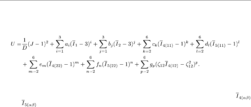
UANISOHYPER_INV
Example: Anisotropic hyperelastic model of Kaliske and Schmidt
As an example of the coding of user subroutine UANISOHYPER_INV, consider the model proposed by
Kaliske and Schmidt (2005) for nonlinear anisotro pic el ast icity w i th two families of fibers. The strain
energy fu nction is given by a polynomial series expansion in the form
The code in user subroutine UANISOHYPER_INV must re tur n the derivatives of the strain energy
function with respect to the scalar invariants, which are readily computed from the above expression. In
this example auxiliary function s are used to facilitate enumeration of pseudo-invariants of type
and , as wel l a s for indexing into the ar ray of second d erivatives using symmetric storage. The
user subroutine would be coded as follows:
subroutine uanisohyper_inv (aInv, ua, zeta, nFibers, nInv,
* ui1, ui2, ui3, temp, noel,
* cmname, incmpFlag, ihybFlag,
* numStatev, statev,
* numFieldv, fieldv, fieldvInc,
* numProps, props)
C
include 'aba_param.inc'
C
character *80 cmname
dimension aInv(nInv), ua(2), zeta(nFibers*(nFibers-1)/2)
dimension ui1(nInv), ui2(nInv*(nInv+1)/2)
dimension ui3(nInv*(nInv+1)/2), statev(numStatev)
dimension fieldv(numFieldv), fieldvInc(numFieldv)
dimension props(numProps)
C
parameter ( zero = 0.d0,
* one = 1.d0,
* two = 2.d0,
* three = 3.d0,
* four = 4.d0,
* five = 5.d0,
* six = 6.d0 )
C
1.1.20–6
Abaqus ID:
Printed on:
UANISOHYPER_INV
C Kaliske-Schmidtt energy function (3D)
C
C Read material properties
d=props(1)
dInv = one / d
a1=props(2)
a2=props(3)
a3=props(4)
b1=props(5)
b2=props(6)
b3=props(7)
c2=props(8)
c3=props(9)
c4=props(10)
c5=props(11)
c6=props(12)
d2=props(13)
d3=props(14)
d4=props(15)
d5=props(16)
d6=props(17)
e2=props(18)
e3=props(19)
e4=props(20)
e5=props(21)
e6=props(22)
f2=props(23)
f3=props(24)
f4=props(25)
f5=props(26)
f6=props(27)
g2=props(28)
g3=props(29)
g4=props(30)
g5=props(31)
g6=props(32)
C
C Compute Udev and 1st and 2nd derivatives w.r.t invariants
C-I1
bi1 = aInv(1)
term = bi1-three
ua(2) = a1*term + a2*term**2 + a3*term**3
1.1.20–7
Abaqus ID:
Printed on:
UANISOHYPER_INV
ui1(1) = a1 + two*a2*term + three*a3*term**2
ui2(indx(1,1)) = two*a2 + three*two*a3*term
C-I2
bi2 = aInv(2)
term = bi2-three
ua(2) = ua(2) + b1*term + b2*term**2 + b3*term**3
ui1(2) = b1 + two*b2*term + three*b3*term**2
ui2(indx(2,2)) = two*b2 + three*two*b3*term
C - I3 (=J)
bi3 = aInv(3)
term = bi3-one
ui1(3) = two*dInv*term
ui2(indx(3,3)) = two*dInv
C - I4(11)
nI411 = indxInv4(1,1)
bi411 = aInv(nI411)
term = bi411-one
ua(2) = ua(2)
* + c2*term**2 + c3*term**3 + c4*term**4
* + c5*term**5 + c6*term**6
ui1(nI411) =
* two*c2*term
* + three*c3*term**2
* + four*c4*term**3
* + five*c5*term**4
* + six*c6*term**5
ui2(indx(nI411,nI411)) =
* two*c2
* + three*two*c3*term
* + four*three*c4*term**2
* + five*four*c5*term**3
* + six*five*c6*term**4
C - I5(11)
nI511 = indxInv5(1,1)
bi511 = aInv(nI511)
term = bi511-one
ua(2) = ua(2)
* + d2*term**2 + d3*term**3 + d4*term**4
* + d5*term**5 + d6*term**6
ui1(nI511) =
* two*d2*term
* + three*d3*term**2
1.1.20–8
Abaqus ID:
Printed on:
UANISOHYPER_INV
* + four*d4*term**3
* + five*d5*term**4
* + six*d6*term**5
ui2(indx(nI511,nI511)) =
* two*d2
* + three*two*d3*term
* + four*three*d4*term**2
* + five*four*d5*term**3
* + six*five*d6*term**4
C - I4(22)
nI422 = indxInv4(2,2)
bi422 = aInv(nI422)
term = bi422-one
ua(2) = ua(2)
* + e2*term**2 + e3*term**3 + e4*term**4
* + e5*term**5 + e6*term**6
ui1(nI422) =
* two*e2*term
* + three*e3*term**2
* + four*e4*term**3
* + five*e5*term**4
* + six*e6*term**5
ui2(indx(nI422,nI422)) =
* two*e2
* + three*two*e3*term
* + four*three*e4*term**2
* + five*four*e5*term**3
* + six*five*e6*term**4
C - I5(22)
nI522 = indxInv5(2,2)
bi522 = aInv(nI522)
term = bi522-one
ua(2) = ua(2)
* + f2*term**2 + f3*term**3 + f4*term**4
* + f5*term**5 + f6*term**6
ui1(nI522) =
* two*f2*term
* + three*f3*term**2
* + four*f4*term**3
* + five*f5*term**4
* + six*f6*term**5
ui2(indx(nI522,nI522)) =
1.1.20–9
Abaqus ID:
Printed on:
UANISOHYPER_INV
* two*f2
* + three*two*f3*term
* + four*three*f4*term**2
* + five*four*f5*term**3
* + six*five*f6*term**4
C - I4(12)
nI412 = indxInv4(1,2)
bi412 = aInv(nI412)
term = zeta(1)*(bi412-zeta(1))
ua(2) = ua(2)
* + g2*term**2 + g3*term**3
* + g4*term**4 + g5*term**5
* + g6*term**6
ui1(nI412) = zeta(1) * (
* two*g2*term
* + three*g3*term**2
* + four*g4*term**3
* + five*g5*term**4
* + six*g6*term**5 )
ui2(indx(nI412,nI412)) = zeta(1)**2 * (
* two*g2
* + three*two*g3*term
* + four*three*g4*term**2
* + five*four*g5*term**3
* + six*five*g6*term**4 )
C
C Add volumetric energy
C
term = aInv(3) - one
ua(1) = ua(2) + dInv*term*term
C
return
end
C
C Maps index from Square to Triangular storage of symmetric
C matrix
C
integer function indx( i, j )
C
include 'aba_param.inc'
C
ii = min(i,j)
1.1.20–10
Abaqus ID:
Printed on:
UANISOHYPER_INV
jj = max(i,j)
C
indx = ii + jj*(jj-1)/2
C
return
end
C
C
C Generate enumeration of Anisotropic Pseudo Invariants of
C type 4
C
integer function indxInv4( i, j )
C
include 'aba_param.inc'
C
ii = min(i,j)
jj = max(i,j)
C
indxInv4=4+jj*(jj-1) + 2*(ii-1)
C
return
end
C
C
C Generate enumeration of Anisotropic Pseudo Invariants of
C type 5
C
integer function indxInv5( i, j )
C
include 'aba_param.inc'
C
ii = min(i,j)
jj = max(i,j)
C
indxInv5=5+jj*(jj-1) + 2*(ii-1)
C
return
end
1.1.20–11
Abaqus ID:
Printed on:

UANISOHYPER_INV
Additional reference
•
Kaliske, M., a nd J. Schmidt, “F ormulation of Fi nit e Nonlinear Anisotropi c Elasticity,” CADFEM
GmbH Infoplaner 2/2 005 , vol. 2, pp. 22–23, 2005.
1.1.20–12
Abaqus ID:
Printed on:

UANISOHYPER_STRAIN
1.1.21 UANISOHYPER_STRAIN: User subroutine to define anisotropic hyperelastic
material behavior based on Green strain.
Product:
Abaqus/Standard
References
•
“Anisotropic hyperelastic behavior,” Section 22.5.3 of the Abaqus Analysis User’s Guide
• *
ANISOTROPIC HYPERELASTIC
•
“UANISOHYPER_INV and VUANISOHYPER_INV,” Section 4.1.13 of the Abaqus Verification
Guide
Overview
User subroutine UANISOHYPER_STRAIN:
•
can be used to define the strain energy potential of anisotropic hyperelastic materials as a function
of the com po nents of the Green strain tenso r;
•
is called at all material calculation points of elem ents for which the material definition contains
user-defined anisotropic hyperelastic behavior with a Green strain-based formu lation (“Anisotropic
hyperelastic behavior,” Section 22.5.3 of the Ab aqus Analysis User’s Guide);
•
can include material behavior dependent on field variables or state variables;
•
requires that the values of th e derivativ es of the strain energy density function of the anisotropic
hyperelastic ma ter ial b e defined with respect to the components of the modifi ed Green strain tensor;
and
•
is called twice per m aterial point in each iteration.
Storage of strain components
In the array of modified Green strain, EBAR, direct components are stored first, followed by shear
components. There are NDI direct and NSHR tensor shear compo nents. The order of the comp onen ts
is de fined in “Conventions,” Section 1.2.2 of the AbaqusAnalysisUser’sGuide. Sincethenumberof
active stress and strain components varies between elem ent types, the routine must be coded to provid e
for all element types with which it will be used.
Storage of arrays of derivatives of the energy function
The array of first derivatives of the strain energy function, DU1, contains NTENS+1 components, with
NTENS=NDI+NSHR.Thefirst NTENS com ponents correspond to the derivatives with respect to each
component of the modified Green strain,
. The last compon ent contains the derivative with
respect to the vol ume r atio,
.
1.1.21–1
Abaqus ID:
Printed on:

UANISOHYPER_STRAIN
The array of second derivatives of the strain energy function, DU2,contains
(NTENS+1)*(NTENS+2)/2 components. These components are ordered using the follow ing
triangular storage scheme:
Component 2D Case 3D Case
1
2
3
4
5
6
7
8
9
10
11
12
13
14
15
16
17
18
19
20
21
22
23
24
1.1.21–2
Abaqus ID:
Printed on:

UANISOHYPER_STRAIN
Component 2D Case 3D Case
25
26
27
28
Finally, the array of third derivatives of the strain energy fun ction, DU3, also contains
(NTENS+1)*(NTENS+2)/2 components, each representing the derivative with respect to
of the
corresponding component of DU2. It follows the same triangular storage scheme as DU2.
Special considerations for various element types
There are several special considerations that need to be noted.
Shells that calculate transverse shear energy
When UANISOHYPER_STRAIN is used to define the material response of shell elements that calculate
transverse shear energy, Abaqus/Standard cannot calculate a default value for the transverse shear
stiffness of the element. Hence, you must define the element’s transverse shear stiffness. See “Shell
section behavior,” Section 29.6.4 of the Abaqus Analysis User’s Guide, for guid e lin es on choosing this
stiffness.
Elements with hourglassing modes
When UANISOHYPER_STRAIN is used to define the material response of elements with hourglassing
modes, you must define the hourglass stiffness for hourglass control based on t he total stiffness approach.
The hourglass stiffness is not requ ir ed for enhanced hourglass control, b ut yo u can define a scaling factor
for the stiffness associated with the drill degree of freedom (rotation abo ut the surface normal). See
“Section controls,” Section 27.1.4 of the Abaqus Analysis User’s Guide.
User subroutine interface
SUBROUTINE UANISOHYPER_STRAIN (EBAR, AJ, UA, DU1, DU2, DU3,
1 TEMP, NOEL, CMNAME, INCMPFLAG, IHYBFLAG, NDI, NSHR, NTENS,
2 NUMSTATEV, STATEV, NUMFIELDV, FIELDV, FIELDVINC,
3 NUMPROPS, PROPS)
C
INCLUDE 'ABA_PARAM.INC'
C
CHARACTER*80 CMNAME
C
DIMENSION EBAR(NTENS), UA(2), DU1(NTENS+1),
1.1.21–3
Abaqus ID:
Printed on:

UANISOHYPER_STRAIN
2 DU2((NTENS+1)*(NTENS+2)/2),
3 DU3((NTENS+1)*(NTENS+2)/2),
4 STATEV(NUMSTATEV), FIELDV(NUMFIELDV),
5 FIELDVINC(NUMFIELDV), PROPS(NUMPROPS)
user coding to define UA,DU1,DU2,DU3,STATEV
RETURN
END
Variables to be defined
UA(1)
U, strain energy density function. For a compressible material at least one derivative involving J should
be nonzero. For an incompressible material a ll derivatives involving J are ignored.
UA(2)
, the devi ator ic part of the s trai n energy density of the primary material response. T his quantity
is needed only if the cur ren t material definition also includes Mullins effect (see “Mullins effect,”
Section 22.6.1 of the Abaqus Analysis User’s Guide).
DU1(NTENS+1)
Derivatives of s train energy potential with respect to the components of the modified Green strain
tensor,
, and with re spect to the volume ratio, .
DU2((NTENS+1)*(NTENS+2)/2)
Second derivatives of strain energy potential with respect to the components of the modified Green
strain ten so r and the volume ratio (using triangular storage, as mentioned earlier).
DU3((NTENS+1)*(NTENS+2)/2)
Derivatives with respect to J of the second derivatives of the strain energy potential (using triangular
storage, as mentioned earlier). This quantity is needed only for compressible materials with a hybrid
formulation (when INCMPFLAG =0andIHYBFLAG =1).
STATEV
Array co ntai ning the user-defined solution-dependent s tate variables at t his point. These are supplied a s
values at the start of the increment or as values updated by other user subroutines (see “User subroutines:
overview,” Section 18.1.1 of the Abaqus Analysis User’s Guide) and must be returned as values at the
end o f the increment.
1.1.21–4
Abaqus ID:
Printed on:

UANISOHYPER_STRAIN
Variables passed in for information
TEMP
Current tem perature at this point.
NOEL
Element number.
CMNAME
User-specified material name, left justified.
NDI
Number of direct stress components at this point.
NSHR
Number of shear componen ts at this point.
NTENS
Size of the stress or strain component array (NDI + NSHR).
INCMPFLAG
Incompressibili ty flag defined to be 1 if the material is specified as incompressible or 0 if the material
is speci fied as compressible.
IHYBFLAG
Hybrid formulation flag definedtobe1forhybridelements;0otherwise.
NUMSTATEV
User-defined n umber of solution-dependent s tate variables associated with this material (see
“Allocating space” in “User subroutines: overview,” S ection 18.1.1 of the Abaqus A nalysis User’s
Guide).
NUMFIELDV
Number of field variables.
FIELDV
Array of interpolated values of predefined field variables at this material point at the end of the
increment based on the values read in at the nodes (initial values at the beginning of th e an alysis and
current values during the analysis).
FIELDVINC
Array of increments of predefined field variables at this material point for this increment, including any
values updated by user subroutine USDFLD.
NUMPROPS
Number of material properties entered for this user-defined hyperelastic material.
1.1.21–5
Abaqus ID:
Printed on:

UANISOHYPER_STRAIN
PROPS
Array of material properties entered for this user-defined hyperelastic material.
EBAR(NTENS)
Modified Green strain tensor,
, at the material point at the end of the increment.
AJ
J, determinant of deformation gradient (volume ratio) at the end of the increm ent.
Example: Orthotropic Saint-Venant Kirchhoff model
As a simple example of the coding of user subroutine UANISOHYPER_STRAIN, con sider the
generalization to anisotropic hyperelasticity of the Saint-Venant Kirchhoff model. The strain energy
function of the S aint-Venant Kirchhoff model can be expressed as a quadratic function of the Green
strain tensor,
,as
where i s the fourth -o rder elastici ty tensor. The derivatives of the strain energy funct ion with re spect
to the G reen strain are given as
However, user subroutine UANISOHYPER_STRAIN must return the derivatives of the strain energy
function with respect to the modified Green strain tensor,
, and the volume ratio, J, w hich can be
accomplished easily using the following relationship between
, ,and :
where is the second-order identity tensor. Thus, using the chain rule we find
1.1.21–6
Abaqus ID:
Printed on:

UANISOHYPER_STRAIN
where
and
In this example an auxiliary function is used to facilitate indexin g into a fourth-order symmetric
tensor. The user subroutine would be coded as follows:
subroutine uanisohyper_strain (
* ebar, aj, ua, du1, du2, du3, temp, noel, cmname,
* incmpFlag, ihybFlag, ndi, nshr, ntens,
* numStatev, statev, numFieldv, fieldv, fieldvInc,
* numProps, props)
c
include 'aba_param.inc'
c
dimension ebar(ntens), ua(2), du1(ntens+1)
dimension du2((ntens+1)*(ntens+2)/2)
dimension du3((ntens+1)*(ntens+2)/2)
dimension statev(numStatev), fieldv(numFieldv)
dimension fieldvInc(numFieldv), props(numProps)
c
character*80 cmname
c
parameter ( half = 0.5d0,
$ one = 1.d0,
$ two = 2.d0,
$ third = 1.d0/3.d0,
$ twothds = 2.d0/3.d0,
$ four = 4.d0 )
*
* Orthotropic Saint-Venant Kirchhoff strain energy function (3D)
*
1.1.21–7
Abaqus ID:
Printed on:
UANISOHYPER_STRAIN
D1111=props(1)
D1122=props(2)
D2222=props(3)
D1133=props(4)
D2233=props(5)
D3333=props(6)
D1212=props(7)
D1313=props(8)
D2323=props(9)
*
d2UdE11dE11 = D1111
d2UdE11dE22 = D1122
d2UdE11dE33 = D1133
*
d2UdE22dE11 = d2UdE11dE22
d2UdE22dE22 = D2222
d2UdE22dE33 = D2233
*
d2UdE33dE11 = d2UdE11dE33
d2UdE33dE22 = d2UdE22dE33
d2UdE33dE33 = D3333
*
d2UdE12dE12 = D1212
*
d2UdE13dE13 = D1313
*
d2UdE23dE23 = D2323
*
xpow = exp ( log(aj) * twothds )
detuInv = one / aj
*
E11 = xpow * ebar(1) + half * ( xpow - one )
E22 = xpow * ebar(2) + half * ( xpow - one )
E33 = xpow * ebar(3) + half * ( xpow - one )
E12 = xpow * ebar(4)
E13 = xpow * ebar(5)
E23 = xpow * ebar(6)
*
term1 = twothds * detuInv
dE11Dj = term1 * ( E11 + half )
dE22Dj = term1 * ( E22 + half )
dE33Dj = term1 * ( E33 + half )
1.1.21–8
Abaqus ID:
Printed on:
UANISOHYPER_STRAIN
dE12Dj = term1 * E12
dE13Dj = term1 * E13
dE23Dj = term1 * E23
term2 = - third * detuInv
d2E11DjDj = term2 * dE11Dj
d2E22DjDj = term2 * dE22Dj
d2E33DjDj = term2 * dE33Dj
d2E12DjDj = term2 * dE12Dj
d2E13DjDj = term2 * dE13Dj
d2E23DjDj = term2 * dE23Dj
*
dUdE11 = d2UdE11dE11 * E11
* + d2UdE11dE22 * E22
* + d2UdE11dE33 * E33
dUdE22 = d2UdE22dE11 * E11
* + d2UdE22dE22 * E22
* + d2UdE22dE33 * E33
dUdE33 = d2UdE33dE11 * E11
* + d2UdE33dE22 * E22
* + d2UdE33dE33 * E33
dUdE12 = two * d2UdE12dE12 * E12
dUdE13 = two * d2UdE13dE13 * E13
dUdE23 = two * d2UdE23dE23 * E23
*
U = half * ( E11*dUdE11 + E22*dUdE22 + E33*dUdE33 )
* + E12*dUdE12 + E13*dUdE13 + E23*dUdE23
*
ua(2) = U
ua(1) = ua(2)
*
du1(1) = xpow * dUdE11
du1(2) = xpow * dUdE22
du1(3) = xpow * dUdE33
du1(4) = xpow * dUdE12
du1(5) = xpow * dUdE13
du1(6) = xpow * dUdE23
du1(7) = dUdE11*dE11Dj + dUdE22*dE22Dj + dUdE33*dE33Dj
* + two * ( dUdE12*dE12Dj
* +dUdE13*dE13Dj
* +dUdE23*dE23Dj )
*
xpow2 = xpow * xpow
1.1.21–9
Abaqus ID:
Printed on:
UANISOHYPER_STRAIN
*
du2(indx(1,1)) = xpow2 * d2UdE11dE11
du2(indx(1,2)) = xpow2 * d2UdE11dE22
du2(indx(2,2)) = xpow2 * d2UdE22dE22
du2(indx(1,3)) = xpow2 * d2UdE11dE33
du2(indx(2,3)) = xpow2 * d2UdE22dE33
du2(indx(3,3)) = xpow2 * d2UdE33dE33
du2(indx(1,4)) = zero
du2(indx(2,4)) = zero
du2(indx(3,4)) = zero
du2(indx(4,4)) = xpow2 * d2UdE12dE12
du2(indx(1,5)) = zero
du2(indx(2,5)) = zero
du2(indx(3,5)) = zero
du2(indx(4,5)) = zero
du2(indx(5,5)) = xpow2 * d2UdE13dE13
du2(indx(1,6)) = zero
du2(indx(2,6)) = zero
du2(indx(3,6)) = zero
du2(indx(4,6)) = zero
du2(indx(5,6)) = zero
du2(indx(6,6)) = xpow2 * d2UdE23dE23
*
du2(indx(1,7)) = xpow * ( term1 * dUdE11
* + d2UdE11dE11 * dE11Dj
* + d2UdE11dE22 * dE22Dj
* + d2UdE11dE33 * dE33Dj )
du2(indx(2,7)) = xpow * ( term1 * dUdE22
* + d2UdE22dE11 * dE11Dj
* + d2UdE22dE22 * dE22Dj
* + d2UdE22dE33 * dE33Dj )
du2(indx(3,7)) = xpow * ( term1 * dUdE33
* + d2UdE33dE11 * dE11Dj
* + d2UdE33dE22 * dE22Dj
* + d2UdE33dE33 * dE33Dj )
du2(indx(4,7)) = xpow * ( term1 * dUdE12
* + two * d2UdE12dE12 * dE12Dj )
du2(indx(5,7)) = xpow * ( term1 * dUdE13
* + two * d2UdE13dE13 * dE23Dj )
du2(indx(6,7)) = xpow * ( term1 * dUdE23
* + two * d2UdE23dE23 * dE13Dj )
du2(indx(7,7))= dUdE11*d2E11DjDj
1.1.21–10
Abaqus ID:
Printed on:
UANISOHYPER_STRAIN
* +dUdE22*d2E22DjDj
* +dUdE33*d2E33DjDj
* + two*( dUdE12*d2E12DjDj
* +dUdE13*d2E13DjDj
* +dUdE23*d2E23DjDj)
* + d2UdE11dE11 * dE11Dj * dE11Dj
* + d2UdE22dE22 * dE22Dj * dE22Dj
* + d2UdE33dE33 * dE33Dj * dE33Dj
* + two * ( d2UdE11dE22 * dE11Dj * dE22Dj
* +d2UdE11dE33 * dE11Dj * dE33Dj
* +d2UdE22dE33 * dE22Dj * dE33Dj )
* + four * ( d2UdE12dE12 * dE12Dj * dE12Dj
* +d2UdE13dE13 * dE13Dj * dE13Dj
* +d2UdE23dE23 * dE23Dj * dE23Dj )
*
return
end
*
* Maps index from Square to Triangular storage
* of symmetric matrix
*
integer function indx( i, j )
*
include 'aba_param.inc'
*
ii = min(i,j)
jj = max(i,j)
*
indx = ii + jj*(jj-1)/2
*
return
end
1.1.21–11
Abaqus ID:
Printed on:

UCORR
1.1.22 UCORR: User subroutine to define cross-correlation properties for random
response loading.
Product:
Abaqus/Standard
References
•
“Random response analysis,” Section 6.3.11 of the Abaqus An alysis User’s Guide
• *
CORRELATION
•
“Random respon se to jet noise excitation,” Section 1.4.10 of the Abaqus Benchmarks Guide
Overview
User su bro utine UCORR:
•
can be used to define the coefficients for the cross-correlation matrix in a random response analysis;
•
will be called once for the com bination of any two degrees of freedom with nonzero prescribed
loads for each load case specified as a concentrated or distributed load or once for the combination
of any two excitation directions specified as a base motion;
•
allows correlation coefficients to be defined as a function of n odal coordinates; and
•
ignores any d ata specified outsid e the user su bro utine for the associated cross-correlation m atrix.
Cross-correlation for base motion excitation
The spat ial correlation matri x for base motion excit ation is definedbythecoefficients in user
subroutine UCORR,where
are excitation directions and J corresponds to the Jth frequency function
referenced under load case I.
Cross-correlation for point loads and distributed loads
The spatial correlation matrix of the load is defined as follows. Let b e the load a p plied to degree of
freedom i at node N in load case I, through the use of a concentrated or distributed load. Let J correspond
to the Jth frequency function referenced under load case I. Th e spatial correlation matri x u sed in the
random response analysis for this l oad case is then
where are the coefficients definedinusersubroutineUCORR. Typically the load magnitude
is given as 1.0; therefore, the load definition is simply selecting the non zero terms that will appear in
.
1.1.22–1
Abaqus ID:
Printed on:

UCORR
User subroutine interface
SUBROUTINE UCORR(PSD,CORRR,CORRI,KSTEP,LCASE,JNODE1,JDOF1,
1 JNODE2,JDOF2,COOR1,COOR2)
C
INCLUDE 'ABA_PARAM.INC'
C
DIMENSION COOR1(3),COOR2(3)
CHARACTER*80 PSD
user coding to define CORRR and CORRI
RETURN
END
Variables to be defined
CORRR
Real part of the cross-correlation scaling factor.
CORRI
Imaginary part of the cross-correlation scaling factor.
Variables passed in for information
PSD
User-specified nam e for the frequency function tha t references this correlati on, left justified.
KSTEP
Step number.
LCASE
Load case number, I.
JNODE1
First node involved, N (not used for base motion excitation).
JDOF1
Degree of freedom i at the first node (for concentrated or distributed load excitation) or global excitation
direction i (for base motion excitation).
JNODE2
Second node involved, M (not used for base m otion excitation).
1.1.22–2
Abaqus ID:
Printed on:
UCORR
JDOF2
Degree of freedom j at the second node (for concentrated or distributed load excitation) or global
excitation direction j (for base motion excitation).
COOR1
An array containing the coordinates of the first node (no t used for base motion excitation).
COOR2
An array containing the coordinates of the second nod e (not used for base motion excitation).
1.1.22–3
Abaqus ID:
Printed on:

UCREEPNETWORK
1.1.23 UCREEPNETWORK: User subroutine to define time-dependent behavior (creep) for
models defined within the parallel rheological framework.
Product:
Abaqus/Standard
References
•
“Parallel rheological framework,” Section 22.8.2 of the Abaqus Analysis User’s Guide
•
“Nonlinear large-strain viscoelastici ty with hyperelast icit y,” Section 2.2.8 of the Abaqus
Ver ification Guide
• *
VISCOELASTIC
Overview
User subroutine UCREEPNETWORK:
•
is intended to provide creep law s for nonlinear viscoelastic network s for mod els defined using the
parallel rheological framework (see “Parallel rheological framework,” Section 22.8.2 of the Abaqus
Analysis User’s Guide);
•
can use and update solution-depen dent state variables; and
•
can be used in conjunctionwithusersubroutineUSDFLD to redefine any field variables before they
are passed in.
Model description
Theusersubroutineallowsacreeplawof the following general form to be defined:
where
and
is th e identity tensor,
is the right Cauchy-Green creep strain tensor,
is the equivalen t creep str ain rate,
is the equivalent creep strain,
is the first invariant of ,
is the second invariant of ,
is the determinant of the deformation gradient, ,
1.1.23–1
Abaqus ID:
Printed on:

UCREEPNETWORK
is the Kirchhoff pressure,
is the equivalent deviatoric Kirchhoff stress,
t is the time,
is the temperature, and
FV are field variables.
The left Cauchy-Green strain tensor,
,isdefined as
where is the deformation gradient with volume change eliminated , which is computed using
The user subroutine must define the increment of creep equivalent strain, , as a function of the time
increment,
, and the variables used in the definition of , as well as the derivatives of the equivalent
creep strain increment with respect to those variables. If any solution-dependent state variables are
included in the definition of
, they m ust also be integrated forward in time in this user subroutine.
User subroutine interface
subroutine ucreepnetwork (
C Must be updated
* outputData,
C Can be updated
* statev,
C Information (Read only)
* nOutput,
* nstatv,
* networkid,
* coords,
* temp,
* dtemp,
* nfield,
* predef,
* dpred,
* nprops,
* props,
* i_array,
* niarray,
* r_array,
* nrarray,
* c_array,
1.1.23–2
Abaqus ID:
Printed on:
UCREEPNETWORK
* ncarray)
C
include 'aba_param.inc'
C
parameter( io_creep_equiv_creepinc = 1,
* io_creep_deqcreepinc_deqcreep = 2,
* io_creep_deqcreepinc_dqtild = 3,
* io_creep_deqcreepinc_dinv1crp = 4,
* io_creep_deqcreepinc_dinv1 = 5,
* io_creep_deqcreepinc_dinv2 = 6,
* io_creep_deqcreepinc_ddetf = 7,
* io_creep_deqcreepinc_dpress = 8 )
C
parameter( i_creep_kstep = 1,
* i_creep_kinc = 2,
* i_creep_noel = 3,
* i_creep_npt = 4,
* i_creep_layer = 5,
* i_creep_kspt = 6,
* i_creep_lend = 7 )
C
parameter( ir_creep_step_time = 1,
* ir_creep_total_time = 2,
* ir_creep_creep_time = 3,
* ir_creep_timeinc = 4,
* ir_creep_equiv_creep_strain = 5,
* ir_creep_qtild = 6,
* ir_creep_inv1crp = 7,
* ir_creep_inv1 = 8,
* ir_creep_inv2 = 9,
* ir_creep_detf = 10,
* ir_creep_press = 11 )
C
parameter( ic_creep_material_name=1)
C
dimension
* statev(nstatv),
* predef(nfield),
* dpred(nfield),
* coords(*),
* props(nprops),
* outputData(nOutput),
1.1.23–3
Abaqus ID:
Printed on:

UCREEPNETWORK
* i_array(niarray),
* r_array(nrarray)
character*80 c_array(ncarray)
C
user coding to define outputData(io_creep_equiv_creepinc),
outputData(io_creep_deqcreepinc_deqcreep),
outputData(io_creep_deqcreepinc_dqtild),
outputData(io_creep_deqcreepinc_dinv1crp),
outputData(io_creep_deqcreepinc_dinv1),
outputData(io_creep_deqcreepinc_dinv2),
outputData(io_creep_deqcreepinc_ddetf) and
outputData(io_creep_deqcreepinc_dpress)
return
end
Variables to be defined
outputData(io_creep_equiv_creepinc)
Equivalent creep strain increment,
.
outputData(io_creep_deqcreepinc_deqcreep)
The derivative:
.
outputData(io_creep_deqcreepinc_dqtild)
The derivative:
.
outputData(io_creep_deqcreepinc_dinv1crp)
The derivative:
.
outputData(io_creep_deqcreepinc_dinv1)
The derivative:
.
outputData(io_creep_deqcreepinc_dinv2)
The derivative:
.
outputData(io_creep_deqcreepinc_ddetf)
The derivative:
.
outputData(io_creep_deqcreepinc_dpress)
The derivative:
.
1.1.23–4
Abaqus ID:
Printed on:

UCREEPNETWORK
Variable that can be updated
statev
An array containing the user-defined solution-depen dent state variables at this po int.
Variables passed in for information
nOutput
Size of array outputData.
nstatv
Number of solution-dependent state variables associated with this material.
networkid
Network identification number, which identifies the network for which creep is defined.
coords
An array containing the current coordinates at t his point.
temp
Temperature at the end of the increment.
dtemp
Increment of tem perature.
nfield
Number of field variables.
predef
An array of interpolated values of predefined field variables at this point at the en d of the increment,
based on the values read in at the nodes and, optionally, redefinedinusersubroutineUSDFLD.
dpred
An array of increments of predefined field variables.
nprops
User-specified number of property values associated with this creep model.
props
An array of user-specified property values that are used to define the c reep model.
i_array(i_creep_kstep)
Step number.
i_array(i_creep_kinc)
Increment number.
1.1.23–5
Abaqus ID:
Printed on:

UCREEPNETWORK
i_array(i_creep_noel)
Element number.
i_array(i_creep_npt)
Integration p oint.
i_array(i_creep_layer)
Layernumber(forlayeredsolids).
i_array(i_creep_kspt)
Section point number within the c urren t layer.
i_array(i_creep_lend)
Start/end of increment flag. Th e value of 0 denotes the beginning of th e increment, and the value of 1
denotes the end of the increment.
niarray
Size of array i_array.
r_array(ir_creep_step_time)
Value o f step time at the end of th e increment.
r_array(ir_creep_total_time)
Value of total time at the end of the increment.
r_array(ir_creep_creep_time)
Value of creep time at the end of the increm ent.
r_array(ir_creep_timeinc)
Time increment.
r_array(ir_creep_equiv_creep_strain)
Equivalent creep strain.
r_array(ir_creep_qtild)
Equivalent deviato ric Kirchhoff stress.
r_array(ir_creep_inv1crp)
The first invariant,
, o f the right Cauchy-Green creep strain tensor, .
r_array(ir_creep_inv1)
The first invariant,
, of the left Cauchy-Green strain tensor, .
r_array(ir_creep_inv2)
The second invariant,
, of the left Cauchy-Green strain tensor, .
1.1.23–6
Abaqus ID:
Printed on:

UCREEPNETWORK
r_array(ir_creep_detf)
The determinant o f the deformation gradient,
.
r_array(ir_creep_press)
Kirchhoff pressure.
nrarray
Size of array r_array.
c_array(ic_creep_material_name)
User-specified material nam e, left justified. S om e internal material models are given names starting
with the “ABQ_” character string. To avoid conflict, you should not use “ABQ_” as the leading string
for the material name.
ncarray
Size of array c_array.
Example: Bergstrom-Boyce model
As an examp le of the coding of user su broutine UCREEPNETWORK, consider the Bergstrom- Boyce
model. In this case t he equivalent creep strain rate is expressed as (see “Parallel rheological fram ework,”
Section 22.8.2 of the Abaqus Analysis User’s Guide)
where
and
is the right Cauchy-Green creep strain tensor,
is the equivalent dev iatoric Kirchhoff stress, and
A, m, C,andE are material parameters.
The user subroutine would be coded as fo llo ws:
subroutine ucreepnetwork (
C Must be updated
* outputData,
C Can be updated
* statev,
C Information (Read only)
* nOutput,
* nstatv,
* networkid,
1.1.23–7
Abaqus ID:
Printed on:
UCREEPNETWORK
* coords,
* temp,
* dtemp,
* nfield,
* predef,
* dpred,
* nprops,
* props,
* i_array,
* niarray,
* r_array,
* nrarray,
* c_array,
* ncarray)
C
include 'aba_param.inc'
C
parameter( io_creep_equiv_creepinc = 1,
* io_creep_deqcreepinc_deqcreep = 2,
* io_creep_deqcreepinc_dqtild = 3,
* io_creep_deqcreepinc_dinv1crp = 4,
* io_creep_deqcreepinc_dinv1 = 5,
* io_creep_deqcreepinc_dinv2 = 6,
* io_creep_deqcreepinc_ddetf = 7,
* io_creep_deqcreepinc_dpress = 8 )
C
parameter( i_creep_kstep = 1,
* i_creep_kinc = 2,
* i_creep_noel = 3,
* i_creep_npt = 4,
* i_creep_layer = 5,
* i_creep_kspt = 6,
* i_creep_lend = 7 )
C
parameter( ir_creep_step_time = 1,
* ir_creep_total_time = 2,
* ir_creep_creep_time = 3,
* ir_creep_timeinc = 4,
* ir_creep_equiv_creep_strain = 5,
* ir_creep_qtild = 6,
* ir_creep_inv1crp = 7,
* ir_creep_inv1 = 8,
1.1.23–8
Abaqus ID:
Printed on:
UCREEPNETWORK
* ir_creep_inv2 = 9,
* ir_creep_detf = 10,
* ir_creep_press = 11 )
C
parameter( ic_creep_material_name=1)
C
C model parameters
parameter ( zero=0.0d0,half=0.5d0,one=1.0d0,two=2.0d0,
& three=3.0d0,five=5.0d0,six=6.0d0 )
C
dimension
* statev(nstatv),
* predef(nfield),
* dpred(nfield),
* coords(*),
* props(nprops),
* outputData(nOutput),
* i_array(niarray),
* r_array(nrarray)
character*80 c_array(ncarray)
C
C Bergstrom-Boyce Model
C
A = props(1)
dm = props(2)
C = props(3)
E = props(4)
C
dI1 = r_array(ir_creep_inv1crp)
dLamb = (dI1/three)**half
sigmaB = r_array(ir_creep_qtild)
dt = r_array(ir_creep_timeinc)
C
C deq
deq = dt*A*(dLamb-one+E)**C*sigmaB**dm
C
C d(deq)/(dI1crp)
deqdi1 = deq*C/(dLamb-one+E)/dLamb/six
C
C d(eq)/d(eq)
deqeq = zero
1.1.23–9
Abaqus ID:
Printed on:
UCREEPNETWORK
C
C d(eq)/d(q)
deqdq = dm*dt*A*(dLamb-one+E)**C*sigmaB**(dm-one)
C
C set output
outputData(io_creep_equiv_creepinc) = deq
outputData(io_creep_deqcreepinc_deqcreep) = deqeq
outputData(io_creep_deqcreepinc_dqtild) = deqdq
outputData(io_creep_deqcreepinc_dinv1crp) = deqdi1
outputData(io_creep_deqcreepinc_dinv1) = zero
outputData(io_creep_deqcreepinc_dinv2) = zero
outputData(io_creep_deqcreepinc_ddetf) = zero
outputData(io_creep_deqcreepinc_dpress) = zero
C
return
end
1.1.23–10
Abaqus ID:
Printed on:

UDECURRENT
1.1.24 UDECURRENT: User subroutine to define nonuniform volume current density in an
eddy current or magnetostatic analysis.
Product:
Abaqus/Standard
References
•
“Eddy current analysis,” Section 6.7.5 of the Abaqu s Analysis User’s Gu ide
•
“Magnetostatic analysis,” Section 6.7.6 of the Abaqus Analysis User’s Guide
• *
DECURRENT
Overview
User subroutine UDECURRENT:
•
can be used to defi ne the variation of volume current density vector as a function of position,
time, element number, etc. f or a transient eddy current o r magnetostatic analysis or as a function
of position, excitation frequency, phase, elem ent num ber, etc. for a time-harmonic eddy current
analysis;
•
will be called at each load integration point for each element-based nonuniform volume current
density definition during eddy current or magnetostatic analysis; and
•
ignores any amplitude references that may a ppear with the associated step definition or nonuniform
distributed volume current density definition.
User subroutine interface
subroutine udecurrent (
C Write only -
* bodycurrent,
C Read only -
* predef, coords, nBlock,
* i_array, niarray,
* r_array, nrarray,
* c_array, ncarray )
C
include 'aba_param.inc'
C
dimension bodycurrent(nBlock,*),
* predef(nBlock,2,*),
* coords(nBlock,*),
* i_array(*),
* r_array(*)
1.1.24–1
Abaqus ID:
Printed on:

UDECURRENT
C
character*80 c_array(*)
C
parameter( i_udecurr_kstep = 1,
* i_udecurr_kinc = 2,
* i_udecurr_noel = 3,
* i_udecurr_npt = 4,
* i_udecurr_jltyp = 5,
* i_udecurr_phase = 6,
* i_udecurr_proc = 7,
* i_udecurr_nfld = 8 )
C
parameter( ir_udecurr_time_1 = 1,
* ir_udecurr_time_2 = 2,
* ir_udecurr_time_3=3)
C
parameter( i_jltyp_cj=1)
C
parameter( i_proc_lf_th = 1,
* i_proc_lf_td = 2,
* i_proc_ms = 3 )
C
parameter( i_udecurr_phase_real = 1,
* i_udecurr_phase_imag = 2 )
C
user coding to define bodycurrent
return
end
Variable to be defined
bodycurrent(nBlock,*)
Components of the body current density vector for a block of load integration points. The units are
CL
−2
T
−1
. bodycurrent will be passed into the routine as the vector speci fied as part of the element-
based distributed vo lum e current density definition . If the vecto r is not defi ned, bodycurrent will
be passed in as zero.
Variables passed in for information
predef(2,*)
An array containing values of temperature and all the predefined field variables at the current load
integration point, based on interpolation from the values specified at the nodes. The first value in a
pair, predef(1,*), corresponds to initial values; the second value, predef(2,*), corresponds to
1.1.24–2
Abaqus ID:
Printed on:
UDECURRENT
incremental values of the temperature and field variables. The first entry (for example, predef(1,1)
or predef(2,1)) con tains the temperature; the subsequent entries (for example, predef(1,2) or
predef(2,2) onward) contain the field variables.
coords(nBlock,*)
An array containing the coordinates of the load integration points.
nBlock
Number of load integration points in this block. Curren tly equal to 1.
i_array(i_udecurr_kstep)
Step number.
i_array(i_udecurr_kinc)
Increment number.
i_array(i_udecurr_noel)
Element number.
i_array(i_udecurr_npt)
Load integration point number.
i_array(i_udecurr_jltyp)
Currently equal to 1.
i_array(i_udecurr_phase)
This value is relevant only for a time-harmonic eddy current analysis and is either 1
(i_udecurr_phase_real)or2(i_udecurr_phase_imag), depending on whether the
current call to the user subroutine defines the real (in-phase) or the imaginary (out-of-phase) part
of the volume current density vector.
i_array(i_udecurr_proc)
Equal to 1 for a time-harmonic eddy current procedure, 2 for a transient eddy current procedure, and 3
for a magnetostatic procedure.
i_array(i_udecurr_nfld)
Total number of predefined field variables.
niarray
Size of array i_array. Currently equ a l to 8.
r_array(ir_udecurr_time_1)
Excitationfrequencyincycles/timeforatime-harmonic eddy current analysis; alternatively, the value
of step time at the b eginning of the current increment for a transient eddy current or magnetostatic
analysis.
1.1.24–3
Abaqus ID:
Printed on:
UDECURRENT
r_array(ir_udecurr_time_2)
Excitation frequency in radians/time for a time-harm onic eddy current analysis; alternatively, the value
of total time at the beginning of the current increment for a transient eddy cu rrent or ma gnetostatic
analysis.
r_array(ir_udecurr_time_3)
Time increment for a transient eddy current or magnetostatic analysis.
nrarray
Size of array r_array. Currently equ a l to 3.
c_array(1)
Not used.
ncarray
Size of array c_array(1). Currently equal to 1.
1.1.24–4
Abaqus ID:
Printed on:

UDEMPOTENTIAL
1.1.25 UDEMPOTENTIAL: User subroutine to define nonuniform magnetic vector potential
on a surface in an eddy current or magnetostatic analysis.
Product:
Abaqus/Standard
References
•
“Eddy current analysis,” Section 6.7.5 of the Abaqu s Analysis User’s Gu ide
•
“Magnetostatic analysis,” Section 6.7.6 of the Abaqus Analysis User’s Guide
• *
D EM POTENTIAL
Overview
User subroutine UDEMPOTENTIAL:
•
can be used to define the variation of the magnetic vector potential as a function of position, tim e,
element num ber, etc. for a transient eddy current or magnetostatic analysis or as a function of
position, excitation frequency, ph a se, element number, etc. for a time-harm onic eddy current
analysis;
•
will be called for each surface-based nonuniform electromagnetic potential definition during eddy
current or magnetostatic analysis; and
•
ignores any amplitude references that may a ppear with the associated step definition or nonuniform
distributed electromagnetic potential defi nition.
User subroutine interface
subroutine udempotential (
C Write only -
* vecPot,
C Read only -
* coords, nBlock,
* i_array, niarray,
* r_array, nrarray,
* c_array, ncarray )
C
include 'aba_param.inc'
C
dimension vecPot(nBlock,*),
* coords(nBlock,*),
* i_array(*),
* r_array(*)
C
1.1.25–1
Abaqus ID:
Printed on:

UDEMPOTENTIAL
character*80 c_array(*)
C
parameter( i_udempot_kstep = 1,
* i_udempot_kinc = 2,
* i_udempot_noel = 3,
* i_udempot_currtyp = 4,
* i_udempot_phase = 5,
* i_udempot_proc = 6)
C
parameter( ir_udempot_time_1 = 1,
* ir_udempot_time_2 = 2,
* ir_udempot_time_3=3)
C
parameter( ic_udempot_surf = 1)
C
parameter( i_pottyp_mvp=1)
C
parameter( i_proc_lf_th = 1,
* i_proc_lf_td = 2,
* i_proc_ms = 3 )
C
parameter( i_udempot_phase_real = 1,
* i_udempot_phase_imag = 2 )
C
user coding to define vecPot
return
end
Variable to be defined
vecPot(nBlock,*)
Components of the m agnetic vector potential at a block of surface points. vecPot will be passed into
the routine as the vector specified as part of the surface-based nonuniform magnetic vector potential
definition. If the vector is no t defined, vecPot will be passed in as zero.
Variables passed in for information
coords(nBlock,*)
An array containing the coordinates of a block of surface points.
nBlock
Number of surface p oints in this blo c k. Currently eq ual to 1.
1.1.25–2
Abaqus ID:
Printed on:
UDEMPOTENTIAL
i_array(i_udempot_kstep)
Step number.
i_array(i_udempot_kinc)
Increment number.
i_array(i_udempot_noel)
Element number.
i_array(i_udempot_pottyp)
Currently equal to 1.
i_array(i_udempot_phase)
This value is relevant only for a time-harmonic eddy current analysis and is either 1
(i_udempot_phase_real)or2(i_udempot_phase_imag), depending on whether the
current call to the user subroutine defines the real (in-phase) or t he imaginary (out-of-phase) part of
the magnetic vector potential.
i_array(i_udempot_proc)
Equal to 1 for a time-harmonic eddy current procedure, 2 for a transient eddy current procedure, and 3
for a magnetostatic procedure.
niarray
Size of array i_array. Currently equ a l to 6.
r_array(ir_udempot_time_1)
Excitationfrequencyincycles/timeforatime-harmonic eddy current analysis; alternatively, the value
of step time at the b eginning of the current increment for a transient eddy current or magnetostatic
analysis.
r_array(ir_udempot_time_2)
Excitation frequency in radians/time for a time-harm onic eddy current analysis; alternatively, the value
of total time at the beginning of the current increment for a transient eddy cu rrent or ma gnetostatic
analysis.
r_array(ir_udempot_time_3)
Time increment for a transient eddy current or magnetostatic analysis.
nrarray
Size of array r_array. Currently equ a l to 3.
c_array(ic_udempot_surf)
Surface name.
1.1.25–3
Abaqus ID:
Printed on:
UDEMPOTENTIAL
ncarray
Size of array c_array. Currently equ a l to 1.
1.1.25–4
Abaqus ID:
Printed on:

UDMGINI
1.1.26 UDMGINI: User subroutine to define the damage initiation criterion.
Product:
Abaqus/Standard
References
•
“Progressive damage and f ailure,” Section 24.1.1 of the Abaqus Analysis User’s Guide
•
“Modeling discontinuities as an enriched feature u sing the extended finite element method,”
Section 10.7.1 of the Abaqus Analysis User’s G uide
• *
DAMAGE INITIATION
Overview
User subroutine UDMGINI:
•
can be used to specify a user-defined damage initiatio n criter io n ;
•
allows the specificatio n of more than one failure m echanism in a n element, with the most severe
one g overning the actual failure;
•
can be used in combination with several Abaqus built-in damage evolution m odels, with each m odel
corresponding to a particular failure mechanism;
•
will be called at all integratio n points of elements for which the ma ter ial definition contains user-
defined damage initiation criterion;
•
can call utility routine GETVRM to access material point data; and
•
is currentl y available o nly for enri c hed elements.
User subroutine interface
SUBROUTINE UDMGINI(FINDEX,NFINDEX,FNORMAL,NDI,NSHR,NTENS,PROPS,
1 NPROPS,STATEV,NSTATEV,STRESS,STRAIN,STRAINEE,LXFEM,TIME,
2 DTIME,TEMP,DTEMP,PREDEF,DPRED,NFIELD,COORDS,NOEL,NPT,LAYER,
3 KSPT,KSTEP,KINC,KDIRCYC,KCYCLELCF,TIMECYC,SSE,SPD,SCD,SVD,
4 SMD,JMAC,JMATYP,MATLAYO,LACCFLA,CELENT,DROT,ORI)
C
INCLUDE 'ABA_PARAM.INC'
C
DIMENSION FINDEX(NFINDEX),FNORMAL(NDI,NFINDEX),COORDS(*),
1 STRESS(NTENS),STRAIN(NTENS),STRAINEE(NTENS),PROPS(NPROPS),
2 STATEV(NSTATV),PREDEF(NFIELD),DPRED(NFIELD),TIME(2),JMAC(*),
3 JMATYP(*),DROT(3,3),ORI(3,3)
1.1.26–1
Abaqus ID:
Printed on:

UDMGINI
user coding to define FINDEX, and FNORMAL
RETURN
END
Variables to be defined
FINDEX(NFINDEX)
A Vector defining the indices fo r all the failure mechanisms.
FNORMAL(NDI, NFINDEX)
An Array defining the normal direction to the fracture plane (three dimensions) or line (two dimensions)
for each failure mechanism.
Variables that can be updated
STATEV
An array containing the user-defined solution-dependent state variables at this point. This array will
be passed in con tain ing the values o f these variables at the start of the increment unless the values
are updated in user subroutine USDFLD. They can be updated in this subroutin e to their values at
the end of the increment. You define the size of this array by allocating space for it (see “Allocating
space” in “User subroutines: overview,” Section 18.1.1 of the Abaqus Analysis User’s Guide, for more
information).
SSE,SPD,SCD,SVD,SMD
Specific elastic strain energy, plastic dissipation, “creep” dissipation, viscous, and damage energy,
respectively, passed in as the v alues at the start of the increment and should be upd ated to the
corresponding specific energy values at the end of the increment. They have no effect on the solution,
except that they are used for energy ou tpu t.
Variables passed in for information
NFINDEX
Number of indices for all failure mechanisms.
NDI
Number of direct stress components at this point.
NSHR
Number of engineering shear stress components at this point.
NTENS
Size of the stress or strain component array (NRI + NSHR).
PROPS(NPROPS)
User-specified array of material constants associated with this user-defined failure criterion.
1.1.26–2
Abaqus ID:
Printed on:
UDMGINI
NPROPS
User-defined n umber of material constants associated with this user-defined failure criterion.
NSTATV
Number of solution-dependent state variab les associated with this material (specified when space is
allocated for the array; see “Allocating space” in “U ser subroutines: overview,” Section 18.1.1 of the
Abaqus Analysis User’s Guide).
STRESS(NTENS)
An Array p assed in as the current stress tensor. If a local orientation is used at the same point as user
subroutine UDMGINI, the stress components will be in the local orientation; in the case of finite-strain
analysis, the basis system in which stress components a re stored rotates with the material.
STRAIN(NTENS)
An Array containing the current total strains. If a local orientation is used at the same point as user
subroutine UDMGINI, the strain compo nents will be in th e local orientation; in the case of finite-strain
analysis, the basis system in w hi ch strain components are stor ed rotates with the mater ial.
STRAINEE(NTENS)
An Array containing the current elastic strains. If a lo cal orientatio n is used at the same point as user
subroutine UDMGINI, the elastic strain components will be in the local orientation; in the case of finite-
strain analysis, the basis system in which elastic strain componen ts are stored rotates w ith the material.
LXFEM
An integer flag to indicate an enriched elem e nt .
TIME(1)
Value of step t ime at the begin nin g of the current increment.
TIME(2)
Value of total time at the beginning of the current increment.
DTIME
Time increment.
TEMP
Temperature at the start of the increm ent.
DTEMP
Increment of temperature during the time increment.
PREDEF
An array containing the values of all o f the user-specified predefi ned variables at this po int at the start
of the increm e nt.
1.1.26–3
Abaqus ID:
Printed on:
UDMGINI
DPRED
An array containing the increments of all of the predefined variables during the time increm ent.
NFIELD
Number of user-specified predefined variables.
COORDS
An array containing the current coordinates of this point.
NOEL
Element number.
NPT
Integration point number.
LAYER
Layer number (for composite shells and layered solids).
KSPT
Section point number within the c urren t layer.
KSTEP
Step number.
KINC
Increment number.
KDIRCYC
Iteration number in a direct cyclic analysis.
KCYCLELCF
Cycle number in a direct cyclic low-cycle fatigue analysis.
TIMECYC
Time period in one loading cycle in a direct cyclic analysis.
JMAC
Variable that must be passed into the GETVRM utility routine to access a material point variable.
JMATYP
Variable that must be passed into the GETVRM utility routine to access a material point variable.
MATLAYO
Variable that must be passed into the GETVRM utility routine to access a material point variable.
LACCFLA
Variable that must be passed into the GETVRM utility routine to access a material point variable.
1.1.26–4
Abaqus ID:
Printed on:

UDMGINI
CELENT
Characteristic element length, which i s a typical length of a line across an element for a first-order
element; it is half of the same typical length for a second-order element. For beams and trusses it is a
characteristic length along the element axis. For membranes and shells it is a characteristic length in
the reference surface. For axisymmetric elements it is a characteristic length in the (r, z) plane only.
For cohesive elem ent s it i s eq ual to the constitutiv e thickness.
DROT(3,3)
Rotation incremen t ma tr ix. This matrix represen ts the i ncrement of rigid bod y rotat ion of the basis
system in which the components of stress (STRESS) and strain (STRAIN) are stored. It is provided
so that vector- or tensor-valued state variables can be rotated a pp ropriately in this subro uti ne: stress
and strain components are already r otated by this amoun t before UDMGINI is called. This matrix is
passed in as a unit matrix for small-displacement analysis and for large-displacement analysis i f the
basis system for the material point rotates with the material (as in a shell element or when a local
orientation is used ).
ORI(3,3)
Material orientation w ith respect to global basis.
Example: User-defined damage initiation criterion with two different failure mechanisms
As a simple example of the coding of user s ubroutine UDMGINI, consider a damage initiation criterion
based on two different failure mechanisms: the maximum principal stress and t he quadratic traction-
interaction.
SUBROUTINE UDMGINI(FINDEX,NFINDEX,FNORMAL,NDI,NSHR,NTENS,PROPS,
1 NPROPS,STATEV,NSTATEV,STRESS,STRAIN,STRAINEE,LXFEM,TIME,
2 DTIME,TEMP,DTEMP,PREDEF,DPRED,NFIELD,COORDS,NOEL,NPT,
3 KLAYER,KSPT,KSTEP,INC,KDIRCYC,KCYCLELCF,TIMECYC,SSE,SPD,
4 SCD,SVD,SMD,JMAC,JMATYP,MATLAYO,LACCFLA,CELENT,DROT,ORI)
C
INCLUDE 'ABA_PARAM.INC'
CC
DIMENSION FINDEX(NFINDEX),FNORMAL(NDI,NFINDEX),COORDS(*),
1 STRESS(NTENS),STRAIN(NTENS),STRAINEE(NTENS),PROPS(NPROPS),
2 STATEV(NSTATEV),PREDEF(NFIELD),DPRED(NFIELD),TIME(2),
3 JMAC(*),JMATYP(*),DROR(3,3),ORI(3,3)
DIMENSION PS(3), AN(3,3), WT(6)
PS(1)=0.0
PS(2)=0.0
PS(3)=0.0
1.1.26–5
Abaqus ID:
Printed on:
UDMGINI
C
C ROTATE THE STRESS TO GLOBAL SYSTEM IF THERE IS ORIENTATION
C
CALL ROTSIG(STRESS,ORI,WT,1,NDI,NSHR)
C
C MAXIMUM PRINCIPAL STRESS CRITERION
C
CALL SPRIND(WT,PS,AN,1,NDI,NSHR)
SIG1 = PS(1)
KMAX=1
DO K1 = 2, NDI
IF(PS(K1).GT.SIG1) THEN
SIG1 = PS(K1)
KMAX = K1
END IF
END DO
FINDEX(1) = SIG1/PROPS(1)
DO K1=1, NDI
FNORMAL(K1,1) = AN(KMAX,K1)
END DO
C
C QUADRATIC TRACTION-INTERACTION CRITERION
c
FINDEX(2)=(STRESS(1)/PROPS(2))**2.0+(STRESS(NDI+1)/
$ PROPS(3))**2.0+(STRESS(NDI+2)/PROPS(4))**2.0
C
FINDEX(2)=sqrt(FINDEX(2))
C
DO K1=1, NDI
FNORMAL(K1,2)=ORI(K1,1)
END DO
RETURN
END
1.1.26–6
Abaqus ID:
Printed on:

UDSECURRENT
1.1.27 UDSECURRENT: User subroutine to define nonuniform surface current density in
an eddy current or magnetostatic analysis.
Product:
Abaqus/Standard
References
•
“Eddy current analysis,” Section 6.7.5 of the Abaqu s Analysis User’s Gu ide
•
“Magnetostatic analysis,” Section 6.7.6 of the Abaqus Analysis User’s Guide
• *
DSECURRENT
Overview
User subro utine UDSECURRENT:
•
can be used to define the variation of surface current density vector as a function of position, time,
element number, load integration point number, etc. for a transient eddy current or magnetostatic
analysis or as a function of position, excitation frequency, phase, element number, load integration
point number, etc. for a time-harmonic eddy current analysis;
•
will be called at each surface load integration point for each nonuniform surface current density
definition during edd y current and magnetostatic analyses; and
•
ignores any amplitude references that may a ppear with the associated step definition or nonuniform
distributed surface current density definition.
User subroutine interface
subroutine udsecurrent (
C Write only -
* surfacecurrent,
C Read only -
* coords, nBlock,
* i_array, niarray,
* r_array, nrarray,
* c_array, ncarray )
C
include 'aba_param.inc'
C
dimension surfacecurrent(nBlock,*),
* coords(nBlock,*),
* i_array(*),
* r_array(*)
C
1.1.27–1
Abaqus ID:
Printed on:

UDSECURRENT
character*80 c_array(*)
C
parameter( i_udsecurr_kstep = 1,
* i_udsecurr_kinc = 2,
* i_udsecurr_noel = 3,
* i_udsecurr_currtyp = 4,
* i_udsecurr_phase = 5,
* i_udsecurr_proc = 6)
C
parameter( ir_udsecurr_time_1 = 1,
* ir_udsecurr_time_2 = 2,
* ir_udsecurr_time_3=3)
C
parameter( ic_udsecurr_surf = 1)
C
parameter( i_currtyp_tangential=1)
C
parameter( i_proc_lf_th = 1,
* i_proc_lf_td = 2,
* i_proc_ms = 3 )
C
parameter( i_udsecurr_phase_real = 1,
* i_udsecurr_phase_imag = 2 )
C
user coding to define surfacecurrent
return
end
Variable to be defined
surfacecurrent(nBlock,*)
Components of the surface current density vector at a block of surface integration points. The
units are CL
−1
T
−1
. surfacecurrent will be passed into the routine as the vector specified as
part of the surface-based distributed surface current density definition. If the vector is not defined,
surfacecurrent will be passed in as zero.
Variables passed in for information
coords(nBlock,*)
An array containing the coordinates of a block of surface load integration points.
1.1.27–2
Abaqus ID:
Printed on:
UDSECURRENT
nBlock
Number of surface integration points in this block. Currently equal to 1 .
i_array(i_udsecurr_kstep)
Step number.
i_array(i_udsecurr_kinc)
Increment number.
i_array(i_udsecurr_noel)
Element number.
i_array(i_udsecurr_currtyp)
Currently equal to 1.
i_array(i_udsecurr_phase)
This value is relevant only for a time-harmonic eddy current analysis and is either 1
(i_udsecurr_phase_real)or2(i_udsecurr_phase_imag), depending on whether the
current call to the user subroutine defines the real (in-phase) or the imaginary (out-of-phase) part
of the surface current density vector.
i_array(i_udsecurr_proc)
Equal to 1 for a time-harmonic eddy current procedure, 2 for a transient eddy current procedure, and 3
for a magnetostatic procedure.
niarray
Size of array i_array. Currently equ a l to 6.
r_array(ir_udsecurr_time_1)
Excitationfrequencyincycles/timeforatime-harmonic eddy current analysis; alternatively, the value
of step time at the b eginning of the current increment for a transient eddy current or magnetostatic
analysis.
r_array(ir_udsecurr_time_2)
Excitation frequency in radians/time for a time-harm onic eddy current analysis; alternatively, the value
of total time at the beginning of the current increment for a transient eddy cu rrent or ma gnetostatic
analysis.
r_array(ir_udsecurr_time_3)
Time increment for a transient eddy current or magnetostatic analysis.
nrarray
Size of array r_array. Currently equ a l to 3.
c_array(ic_udsecurr_surf)
Surface name.
1.1.27–3
Abaqus ID:
Printed on:
UDSECURRENT
ncarray
Size of array c_array. Currently equ a l to 1.
1.1.27–4
Abaqus ID:
Printed on:

UEL
1.1.28 UEL: User subroutine to define an element.
Product:
Abaqus/Standard
WARNING : This feature is intended for advanced users only. Its use in all but the
simplest test examples will require considerable coding by the user/developer.
“User-defined elements,” Section 32.17.1 o f the Abaqus Analysis User’s Guide,
should be read before proceeding.
References
•
“User-defined elements,” Section 32.17.1 of the Abaq us Analysis User’s Guide
• *
UEL PROPERTY
• *
USER ELEMENT
Overview
User subroutine UEL:
•
will be called for each element that is of a general u ser-defined element type (i.e., not defined by
a linear stiffness or mass matrix read either directly or from results file data) each time element
calculations are required; and
•
(or sub rou tines called by user subro utine UEL) must perform all of the calculations for the element,
appropriate to the current activity in the analysis.
Wave kinematic data
For Abaq us/Aq ua applications four utility routines— GETWAVE, GETWAVEVEL, GETWINDVEL,and
GETCURRVEL—are provided to access the fluid kinematic data. T hese routines are u sed from within
user subroutine UEL and are discussed in detail in “Obtaining wave kinematic data in an Abaqus/Aqua
analysis,” Section 2.1.13.
User subroutine interface
SUBROUTINE UEL(RHS,AMATRX,SVARS,ENERGY,NDOFEL,NRHS,NSVARS,
1 PROPS,NPROPS,COORDS,MCRD,NNODE,U,DU,V,A,JTYPE,TIME,DTIME,
2 KSTEP,KINC,JELEM,PARAMS,NDLOAD,JDLTYP,ADLMAG,PREDEF,NPREDF,
3 LFLAGS,MLVARX,DDLMAG,MDLOAD,PNEWDT,JPROPS,NJPROP,PERIOD)
C
INCLUDE 'ABA_PARAM.INC'
C
DIMENSION RHS(MLVARX,*),AMATRX(NDOFEL,NDOFEL),PROPS(*),
1 SVARS(*),ENERGY(8),COORDS(MCRD,NNODE),U(NDOFEL),
1.1.28–1
Abaqus ID:
Printed on:

UEL
2 DU(MLVARX,*),V(NDOFEL),A(NDOFEL),TIME(2),PARAMS(*),
3 JDLTYP(MDLOAD,*),ADLMAG(MDLOAD,*),DDLMAG(MDLOAD,*),
4 PREDEF(2,NPREDF,NNODE),LFLAGS(*),JPROPS(*)
user coding to define RHS, AMATRX, SVARS, ENERGY, and PNEWDT
RETURN
END
Variables to be defined
These arrays depend on the value of the LFLAGS array.
RHS
An array containing the contributions of this element to the right-hand-side vectors of the overall system
of eq uations. For most nonlinear analysis procedures, NRHS=1 and RHS sho uld co ntain the residual
vector. The exception is the modified Riks static procedure (“Static stress analysis,” Section 6.2.2 of
theAbaqusAnalysisUser’sGuide),forwhichNRHS=2 and the first column in RHS should contain the
residual vector and the second column should contain the increments of externa l load on the element.
RHS(K1,K2) is the entry for the K1th degree of freedom of the element in the K2th right- hand-side
vector.
AMATRX
An array containing the contribution of this element to the Jacobian (stiffness) or other m atrix of the
overall system o f equations. T he particular matrix required at any time depends on th e entries in the
LFLAGS array (see below).
All nonzero entries in AMATRX should be defined, even if the matrix is symm etric. If you do
not specify that the matrix is unsymm e tric when you define the user element, Abaqus/Standard will
use the symmetric m a tr ix d e fined by
,where is the m atrix defined as AMATRX
in this subroutine. If you specify that the matrix is unsymmetric when you define the user element,
Abaqus/Standard will use AMATRX directly.
SVARS
An array containing the values of the solution-dependent state variables associated with this element.
The number of such variables is NSVARS (see below). You define the meaning of these variables.
For g eneral nonlinear steps this array is passed into UEL containing the values of these variables at
the start of the current increment. Th ey shoul d be updated to be the values at the end of the increment,
unless the proced ure during which UEL is being called does not require s uch an update. This depends
on the e ntries in th e LFLAGS array (see below). For linear perturbation steps this array is passed into
UEL containing the values of these variables in the base state. They should be returned containing
perturbation values if you wish to output such quantities.
1.1.28–2
Abaqus ID:
Printed on:

UEL
When KINC is equal to zero, the call to UEL is made for zero increment output (see “Output,”
Section 4.1.1 of the Abaqus Analysis User’s Guid e). In this case the values returned will be used only
for output purposes and a re not updated p erm a nen tly.
ENERGY
For general nonlinear steps array ENERGY contains the values of the energy quantities asso ciated w ith
the element. The values in this array when UEL is called are the element energy quantities at th e start
of the current increm ent. They should be updated to the values at the end of the current increment.
For linear perturbation steps th e array is passed into UEL containing the energy in the base state. They
should be returned con tain ing perturbation value s i f you wish to output such quantities. The entries in
the array are as f ollows:
ENERGY(1) Kinetic energy.
ENERGY(2) Elastic strain energy.
ENERGY(3) Creep dissipation.
ENERGY(4) Plastic dissipation.
ENERGY(5) Viscous dissipatio n.
ENERGY(6) “Artificial strain energy” associated with such effects as artificial
stiffness introduced to control hourglassing or other singular modes
in the element.
ENERGY(7) Electrostatic energy.
ENERGY(8) Incremental work done by loads applied within the user element.
When KINC is equal to zero, the call to UEL is made for zero increment output (see “Output,”
Section 4.1.1 of the Abaq us Analysis User’s G uide). In this case the energy values returned will be
used only for output purp oses and are not updated permanently.
Variable that can be updated
PNEWDT
Ratio of suggested n ew time increment to the time increment currently bein g used (DTIME,see
below). This variable allows you to provide input to the automatic tim e increm ent a tion algorithms in
Abaqus/Standard (if auto mat ic time incre men tati on is cho sen). It is useful only during equilibrium
iterations with the normal time increment ation, as indicated by LFLAGS(3)=1.Duringasevere
discontinuity iteration (such as con tact changes), PNEWDT is ignored u nless CONV ERT SDI=YES is
specified for this step. The usage of PNEWDT is discussed below.
PNEWDT is set to a large value before each call to UEL.
If PNEWDT is redefined to be less than 1.0, A baq us/Stan dard must aban don the time increment
and attempt it again with a smaller time increment. The suggested n ew time increment provided to the
automatic time integration algorithms is PNEWDT × DTIME,wherethePNEWDT used is the minimum
value fo r all calls to user subrou tines that allow redefinition of PNEWDT for this iter a tion.
1.1.28–3
Abaqus ID:
Printed on:

UEL
If PNEWDT is given a value that is greater than 1.0 f or all calls to user subroutines for this iteration
and the increment converges in this iteration, Abaqus/Standard m ay increase the time increment. The
suggested new time i ncr ement provided to the automati c time integration algorithms is PNEWDT ×
DTIME,wherethePNEWDT used is the minimum value for all calls to user sub routines for this itera tio n.
If automatic time i ncrementation is not selected in the analysis procedure, values of PNEWDT that
are greater than 1.0 will be ignored and values of PNEWDT that are less than 1.0 will cause the job to
terminate.
Variables passed in for information
Arrays:
PROPS
A floating point array co ntaining the NPROPS real property values defined for use with this element.
NPROPS is the user-specified number of real property values. See “Defining the elem ent properties”
in “User -de fined elements,” Section 32.17.1 of the Abaqus Analysis User’s Guide.
JPROPS
An integer array containing the NJPROP integer property values defined for use with this element.
NJPROP is the user-specified number of integer property values. See “Definin g the element prop erties”
in “User -de fined elements,” Section 32.17.1 of the Abaqus Analysis User’s Guide.
COORDS
An array contain ing the original coordinates of the nodes of the elem ent. COORDS(K1,K2) is the
K1th coordinate of the K2th node of the element.
U, DU, V, A
Arrays containing the current estimates of the basic solution variab les (displacements, rotations,
temperatures, depending on the degree of freedom) at th e nodes of the element at the end of the
current increment. Values are provided as follows:
U(K1) Total values o f the variables. If this is a linear perturbation step, it is
the value in the base state.
DU(K1,KRHS) Incremental values of the variables for the current increment for
right-hand-side KRHS. If this is an eigenvalue extraction step, this is
the eigenvector magnitude for eigenvector KRHS. For steady-state
dynamics, KRHS
denotes real comp onents of perturbation
displacement and KRHS
denotes imaginary components of
perturbation displacement.
V(K1) Time rate of ch ange of the variables (velocities, rates of rotation).
Defined f or implicit dynamics only (LFLAGS(1)
11 or 12).
A(K1) Accelerations of the variables. Defined for implicit dynamics only
(LFLAGS(1)
11 or 12).
1.1.28–4
Abaqus ID:
Printed on:

UEL
JDLTYP
An array containing the integers used to define distribu ted load types for the element. Loads of type
Un are i dentified by the integer value n in JDLTYP; loads of type UnNU are identified by the negative
integer value
in JDLTYP. JDLTYP(K1,K2) is the identifier of the K1th distribut ed load in the
K2th load case. For general nonlinear steps K2 is always 1.
ADLMAG
For general nonlinear steps ADLMAG(K1,1) is the total load magnitude of the K1th distributed load at
the end of the current increment fo r d istribu ted loads of type U n. For distributed loads of typ e UnNU,
the load mag nitude is defined in UEL; therefore, the corresponding entries in ADLMAG are zero. For
linear perturbation step s ADLMAG(K1,1) contains the total load magnitude of the K1th distributed
load of type Un applied in the base state. Base state loading of type Un NU must be dealt w ith inside
UEL. ADLMAG(K1,2), ADLMAG(K1,3), etc. are currently not used.
DDLMAG
For general nonlinear steps DDLMAG contains the increments in t he magnitudes of the distributed loads
that are currentl y active on thi s element for d istr ibu ted loads of type Un. DDLMAG(K1,1) is the
increment of magnitude o f the l oad f or th e current time increment. The increment of load magnitude
is needed to compute the external w ork contribution. For d istr ibuted loads of type UnNU, the load
magnitude is defined in UEL; therefore, the corresp onding entries in DDLMAG are zero. For linear
perturbation steps DDLMAG(K1,K2) contains the perturbation in the mag nitudes of the distributed
loads that are currently active on this element for d istr ibuted loads of typ e Un. K1 denotes the K1th
perturbation load active on the element. K2 is always 1, except for steady-state dynamics, where K2=1
for real loads and K2=2 for imag inary loads. Perturbation loads of type UnNU must be dealt with
inside UEL.
PREDEF
An array containing the values of predefined field variables, such as temperature in an uncoupled
stress/displacement analysis, at the nodes of the element (“Predefined
fields,” Section 34.6.1 of the
Abaqus Analysis User’s Guide).
The first index of the array, K1, is either 1 or 2, with 1 indicating the value of the field variable
at the end of the increment and 2 indicating the increment in the field variable. The second index,
K2, indicates the variable: the temperature co rresp onds to i ndex 1, and the predefined field variables
correspond to indices 2 and above. In cases where temperature is not defined, the predefined fi eld
variables begin with index 1. The third index, K3, indicates the local node number on the element.
PREDEF(K1,1,K3) Temperature.
PREDEF(K1,2,K3) First predefi ned field variable.
PREDEF(K1,3,K3) Second predefined field v ariable.
Etc. Any other predefined field variable.
1.1.28–5
Abaqus ID:
Printed on:

UEL
PREDEF(K1,K2,K3) Total or incremental value of the K2th predefined field variable
at the K3th node of the element.
PREDEF(1,K2,K3) Values of the variables at the end of the current increment.
PREDEF(2,K2,K3) Incremental values correspon ding to the current time
increment.
PARAMS
An array containing the param eters associated with the solution procedure. The entries in this array
depend on the solution procedure currently being used when UEL is called, as indicated by the entries
in the LFLAGS array (see below).
For implicit dynamics (LFLAGS(1) =11or12)PARAMS contains the i ntegration operator values,
as:
PARAMS(1)
PARAMS(2)
PARAMS(3)
LFLAGS
An array containing the flags that define the current solution procedu re and requirements for element
calculations. Detailed requirem ents for the various Abaqus/Standard procedures are defined earlier in
this section.
LFLAGS(1) Defines the procedu re type. See “Results file output format,”
Section 5.1.2 of the Abaqus Analysis U ser’s Guide, for the key
used for each procedure.
LFLAGS(2)=0 Small-displacement analysis.
LFLAGS(2)=1 Large-displacement analysis (nonlinear geometric effects
included in th e step; see “General and linear perturbation
procedures,” Section 6.1.3 o f the Abaqu s Analysis U ser’s Guide).
LFLAGS(3)=1 Normal implicit tim e incrementation proced ur e. User subroutine
UEL must define the residual vector in RHS and the Jacobian
matrix in AMATRX.
LFLAGS(3)=2
Define the current stiffness matrix (AMATRX
or )only.
LFLAGS(3)=3 Define the current damping matrix (AMATRX
or ) only.
1.1.28–6
Abaqus ID:
Printed on:

UEL
LFLAGS(3)=4
Define the current mass matrix (AMATRX
) only. Abaqus/Standard always requests an initial
mass matrix at th e s tar t of the analysis.
LFLAGS(3)=5
Define the current residual or l oad vector (RHS
) only.
LFLAGS(3)=6 Define the current mass matrix and t he residual vector for the
initial acceleration calculation (or the calculation of accelerations
after impact).
LFLAGS(3)=100 Define perturbation quantities for output.
LFLAGS(4)=0 The step is a general step.
LFLAGS(4)=1 The step is a linear perturbation step.
LFLAGS(5)=0
The cu rrent approximations to
, etc. were based on Newton
corrections.
LFLAGS(5)=1 The current approximations were found by extrapolation from
the previous increment.
TIME(1)
Current value of step time or frequency.
TIME(2)
Current value of total time.
Scalar parameters:
DTIME
Time increment.
PERIOD
Time period o f the current step.
NDOFEL
Number of degrees of freedom in the element.
MLVARX
Dimensioning parameter used when several displacement or right-hand-side vectors are used.
NRHS
Number of load vectors. NRHS is 1 in most nonlinear pro blems: it is 2 for the modified Riks static
procedure (“Static stress analysis,” Section 6.2.2 of theAbaqusAnalysisUser’sGuide),anditisgreater
than 1 in some linear analysis procedures andduringsubstructure generation.
1.1.28–7
Abaqus ID:
Printed on:
UEL
NSVARS
User-defined n um ber of solution-dependent s tate variables associated with the element (“Defining
the number of solution-d epend ent variables th at must be stored withi n the element” in “User-defined
elements,” Section 32.17.1 of the Abaq us Analysis User’s Guide).
NPROPS
User-defined n um ber of real property values associated with the element (“Defining the element
properties” in “User-defined elements,” Section 32.17.1 of the Abaqus Analysis User’s Guide).
NJPROP
User-defined number o f integer property values associated with the elemen t (“D efin ing the element
properties” in “User-defined elements,” Section 32.17.1 of the Abaqus Analysis User’s Guide).
MCRD
MCRD is defined as the max im um of the user-defined maximum number of coordinates needed at any
node point (“Defining the maximum number of coordin ates needed at any nodal point” in “User-defined
elements,” Section 32.17.1 of the Abaqus Analysis User’s Guide) and the value of the largest active
degree of freedom of the user element that is less than or equal to 3. F or example, if you specify that
the maxim um number of coordinates is 1 and the active degrees of freedom of the user element are 2,
3, and 6, MCRD will be 3. If you specify that the maxim um num ber of coord inates is 2 and the active
degrees of freed om o f the user element are 11 and 12, MCRD will be 2.
NNODE
User-defined number o f n odes on the elem ent (“Defining the number of nodes associated with the
element” in “User-defined elements,” S ection 32.17.1 of the Abaqus Analysis User’s Gu ide).
JTYPE
Integer d e fi ning the element type. T his is the user-defined integ er value n in element type
Un (“Assigning an element type key to a user-defined element” in “User-defined elements,”
Section 32.17.1 of th e Ab aqus Analysis User’s Guide).
KSTEP
Current step number.
KINC
Current i ncrem ent nu mb er.
JELEM
User-assigned elem ent number.
NDLOAD
Identification number of the distributed load or flux currently active on this element.
MDLOAD
Total number of distributed loads and/ or fluxes definedonthiselement.
1.1.28–8
Abaqus ID:
Printed on:
UEL
NPREDF
Number of predefined field variables, including temperature. For user elements Abaqus/Standard uses
one value for each field variable per node.
UEL conventions
The solution variables (displacem ent, velocity, etc.) are arranged on a node/degree of freedom basis.
The degrees of freedom of the first n ode are first, followed b y the degrees of freedom of the second node,
etc.
Usage with general nonlinear procedures
The values of (and, in direct-integration dynamic steps, and ) enter user subroutine UEL as
their latest app roximations at the e nd of the time increment; that is, at time
.
The values of
enter the subroutine as their values at the beg inn ing of the time in crement; that
is, at time t. It is your responsibility to define suitable t im e integration schemes to u pdat e
.To
ensure accurate, stable integration of internal state variables, you can control the time incrementation via
PNEWDT.
The values of
enter th e subroutine as the values of the total load magnitud e for the th distributed
load at the end of the increment. Increments in the load magnitudes are also available.
In the following descriptions of the user element’s requirements, it will be assum e d that
LFLAGS(3)=1 unless otherw ise stated.
Static analysis (LFLAGS(1)=1,2)
•
.
•
Automatic convergence checks are applied to the force residuals corresponding to degrees of
freedom 1–7.
•
You mus t d efine AMATRX and RHS and update the state variables,
.
Modified Riks static analysis (LFLAGS(1)=1)and(NRHS=2)
•
,where , and are fixed load parameters, and is the
Riks (scalar) load parameter.
•
Automatic convergence checks are applied to the force residuals corresponding to degrees of
freedom 1–7.
•
You m ust d efine AMATRX , RHS(1) ,andRHS(2)
and update the state variables, . RHS(2) is the incremental load vector.
Direct-integration dynamic analysis (LFLAGS(1)=11, 12)
•
Automatic convergence checks are applied to the force residuals corresponding to degrees of
freedom 1–7.
1.1.28–9
Abaqus ID:
Printed on:

UEL
•
LFLAGS(3)=1: N ormal time increment. Either t he Hilber-Hughes-Tay lor or the backward Euler
time integ ration scheme will be used. With
set to zero for the backward Euler, both schemes
imply
where and ;thatis,
the highest time derivative of
in and is ,sothat
Therefore, you must store as an internal state vector. If half-increment residual calculations
are required, you must also store
as an internal state vector, where indicates the time at the
beginning of the previous increment. For
, and is not
needed. You must define AMATRX
where and . RHS m ust also be
defined and the state variables,
, updated . Although the valu e of given in the dynam ic step
definition is passed into UEL,thevalueof
can vary from element to element. For example, can
be set to zero for some elements in the model where numerical dissipation is not desired.
•
LFLAGS(3)=5: Half-increm ent residual ( ) calculation. A baqus/Standard will adjust the time
increment so that
(where is specified in the dynamic step
definition). The half-incremen t residu al is defined as
where indicates the time at the beginning of the previous increm ent ( is a param eter of the
Hilber-Hughes-Tay lor time integration operator and will be set to zero if the backward Euler time
integration operator is used). You must define RHS
.Toevaluate and ,you
must calculate
. T h e se half-incremen t valu es will not be saved. DTIME will still cont ain
(not ). The values contained in U, V, A,andDU are half-increment values.
•
LFLAGS(3)=4: Velocity jum p calculation. Abaqus/Standard solves for ,
so you must define AMATRX
.
•
LFLAGS(3)=6: Initial acceleration calculation. Abaqus/Standard solves
for ,soyoumustdefine AMATRX and RHS .
Subspace-based dynamic analysis (LFLAGS(1)=13)
•
The requirements are identical to those of static analysis, except that the Jacobian (stiffness),
AMATRX, is not needed. No convergence checks are performed in this case.
Quasi-static analysis (LFLAGS(1)=21)
•
The requirem ent s are identical to those of static analysis.
1.1.28–10
Abaqus ID:
Printed on:

UEL
Steady-state heat transfer analysis (LFLAGS(1)=31)
•
The requirements are identical to tho s e of static analysis, except that the automatic convergence
checks are applied to the heat flux residuals corresponding to degrees of freedom 11, 12, …
Transient heat transfer analysis ( θ
max
)(LFLAGS(1)=32, 33)
•
Automatic convergence checks are applied to the heat fl ux residuals corresponding to degrees of
freedom 11, 12, …
•
The backward difference scheme is always used fo r time integration; that is, Abaqus/Standard
assumes that
,where and so always. For
degrees of freedom 11, 12, …,
will be compared against the user-prescribed maxim um
allowable nodal tem perature change in an increment,
, for controlling the time integration
accuracy.
•
You need to define AMATRX ,where is the heat capacity m atrix and
RHS
, and m u st update the state variables, .
Geostatic analysis (LFLAGS(1)=61)
•
Identical to static analysis, except that the automatic convergence checks are applied to the residuals
corresponding to degrees of freedom 1–8.
Steady-state coupled pore fluid diffusion/stress analysis (LFLAGS(1)=62, 63)
•
Identical to static analysis, except that the automatic convergence checks are applied to the residuals
corresponding to degrees of freedom 1–8.
Transient coupled pore fluid diffusion/stress (consolidation) analysis ( u
w
max
)(LFLAGS(1)=64,
65)
•
Automatic convergence checks are applied to th e residuals corresponding to degrees of freedom
1–8.
•
The backward difference scheme is used for time integration; that is, ,where
.
•
For degree of freedom 8, will be compared against the user-prescribed maximum
wetting liquid pore p ressur e change,
, for automatic control of the time integration accuracy.
•
You mus t d efine AMATRX ,where is the pore fluid capacity matrix
and RHS
, and must upd ate the state variables, .
Steady-state fully coupled thermal-stress analysis (LFLAGS(1)=71)
•
Identical to static analysis, except that the automatic convergence checks are applied to the residuals
corresponding to degrees of freedom 1–7 and 11, 12, …
1.1.28–11
Abaqus ID:
Printed on:

UEL
Transient fully coupled thermal-stress analysis (
θ
max
)(LFLAGS(1)=72,73)
•
Automatic convergence checks are applied to th e residuals corresponding to degrees of freedom
1–7 and 11, 12, …
•
The backward difference scheme is used for time integration; that is, ,where
.
•
For degrees of freedom 11, 12, … , will be compared against the user-prescribed
maximum allow able nodal temperature change in an increment,
, for automatic control of
the tim e integration accuracy.
•
You m u s t define AMATRX ,where is the heat capacity matrix and
RHS
, and m u st update the state variables, .
Steady-state coupled thermal-electrical analysis (LFLAGS(1)=75)
•
The requirements are identical to tho s e of static analysis, except that the automatic convergence
checks are applied to the current density residuals corresponding to degree of freedom 9, in addition
to the heat flux residuals.
Transient coupled thermal-electrical analysis ( θ
max
)(LFLAGS(1)=76, 77)
•
Automatic convergence checks are applied t o the current density residuals correspondingtodegree
of freed om 9 and to the heat flux residu als corresponding to degree o f freedom 11.
•
The backward difference scheme is always used fo r time integration; that is, Abaqus/Standard
assumes that
,where . Therefore, always. For
degree of freedom 11
will be compared against the user-prescribed maxim um allowable
nodal temperature change in an increment,
, for controlling the time integration accuracy.
•
You m u s t define AMATRX ,where is the heat capacity matrix and
RHS
, and m u st update the state variables, .
Steady-state coupled thermal-electrical-structural analysis (LFLAGS(1)=102)
•
Identical to static analysis, except that the automatic convergence checks are applied to the residuals
corresponding to degrees of freedom 1– 7, 9, and 11.
Transient coupled thermal-electrical-structural analysis ( θ
max
)(LFLAGS(1)=103,104)
•
Automatic convergence checks are applied to th e residuals corresponding to degrees of freedom
1–7, 9, and 11.
•
The backward difference scheme is always used fo r time integration; that is, Abaqus/Standard
assumes that
,where . Therefore, always. For
degree of freedom 11
will be compared against the user-prescribed maxim um allowable
nodal temperature change in an increment,
, for controlling the time integration accuracy.
•
You m u s t define AMATRX ,where is the heat capacity matrix and
RHS
; and you m ust update the state variables, .
1.1.28–12
Abaqus ID:
Printed on:

UEL
Usage with linear perturbation procedures
“General and linear perturbation procedures,” Section 6.1.3 of the Abaqus Analysis User’s Guide,
describes the linear perturbation capabilities i n Abaqus/Standard. Here, base state values of variables
will be denoted by
, , etc. Pertu rbation values will be deno ted by , ,etc.
Abaqus/Standard will not call user subroutine UEL for the eigenvalue buckling prediction
procedure.
For response spectrum, random response, transient m odal dynamic, and mode-based steady-state
dynamic procedures, user subroutine UEL is called only in a prio r natural frequency extraction analysis,
and the mass and stiffness contributions are taken into account during modal superposition.
For direct-solution and mode-based steady-state dynamic, complex eigenvalue extraction, matrix
generation, and substructure generation procedures, Abaqus/Standard will call user s ubrou tin e UEL, but
only m ass and stiffness contributions will be taken into account. The damping contributions will be
neglected.
Static analysis (LFLAGS(1)=1, 2)
•
Abaqus/Standard will solve for ,where is the base s tat e stiffness matrix
and the perturbation load vector,
, is a linear function of the perturbation loads, ;thatis,
.
•
LFLAGS(3)=1: You must define AMATRX and RHS .
•
LFLAGS(3)=100: You must compute perturbations of the internal variables, , and define RHS
for output purposes.
Eigenfrequency extraction analysis (LFLAGS(1)=41)
•
.
•
Abaqus/Standard will solve for and ,where
is the base state stiffness matrix and is the base state mass
matrix.
•
LFLAGS(3)=2:Define AMATRX .
•
LFLAGS(3)=4:Define AMATRX .
Example: Structural and heat transfer user element
Both a structural and a heat transfer user element have been created to demonstrate the usage of subroutine
UEL. These user-defined elements are applied i n a number of analyses. The follo win g excerpt is from
the verification problem that invokes the structural user element in an implicit dynamics procedure:
*
USER ELEMENT, NODES=2, TYPE=U1, PROPERTIES=4, COORDINATES=3,
VARIABLES=12
1, 2, 3
*
ELEMENT, TYPE=U1
101, 101, 102
1.1.28–13
Abaqus ID:
Printed on:
UEL
*
ELGEN, ELSET=UTRUSS
101, 5
*
UEL PROPERTY, ELSET=UTRUSS
0.002, 2.1E11, 0.3, 7200.
The user element consists of two nodes that are assumed to lie paral lel to th e x-axis. The eleme nt
behaves like a linear truss elemen t. The supplied elem ent properties are the cross-sectional area, Young’s
modulus, Poisson’s ratio, and density, respectively.
The next e x cerp t shows the listing of the subroutine. The user subroutine h as been coded for use in
a per turbation static analysis; general static analysis, inclu ding R i ks analy sis wit h load incrementation
defined by the subroutine; eigenfrequency extraction analysis; and direct-integration dynamic analysis.
The names of the verification input files associated with the su br out ine and these p rocedures can be found
in “UEL,” Section 4.1.14 of the Abaqus Verification G uide. The subroutine perform s all calculatio ns
required for the relevant procedures as described earlier in this section. The flagspassedinthroughthe
LFLAGS array are used to associate particular calculations with solution p rocedures.
During a modified Riks analysis all force loads must be passed into UEL by means of distributed
load definitions such that they are av ailab le for the definition of incremental load vectors; the load keys
Un and UnN U must be used properly, as discussed in “User-defined elem ents,” Section 32.17.1 of th e
Abaqus Analysis User’s Guide. The coding in subroutine UEL must distrib ute the loads into consistent
equivalent nodal forces and account for them in the calculation of the RHS and ENERGY arrays.
SUBROUTINE UEL(RHS,AMATRX,SVARS,ENERGY,NDOFEL,NRHS,NSVARS,
1 PROPS,NPROPS,COORDS,MCRD,NNODE,U,DU,V,A,JTYPE,TIME,
2 DTIME,KSTEP,KINC,JELEM,PARAMS,NDLOAD,JDLTYP,ADLMAG,
3 PREDEF,NPREDF,LFLAGS,MLVARX,DDLMAG,MDLOAD,PNEWDT,
4 JPROPS,NJPROP,PERIOD)
C
INCLUDE 'ABA_PARAM.INC'
PARAMETER ( ZERO = 0.D0, HALF = 0.5D0, ONE = 1.D0 )
C
DIMENSION RHS(MLVARX,*),AMATRX(NDOFEL,NDOFEL),
1 SVARS(NSVARS),ENERGY(8),PROPS(*),COORDS(MCRD,NNODE),
2 U(NDOFEL),DU(MLVARX,*),V(NDOFEL),A(NDOFEL),TIME(2),
3 PARAMS(3),JDLTYP(MDLOAD,*),ADLMAG(MDLOAD,*),
4 DDLMAG(MDLOAD,*),PREDEF(2,NPREDF,NNODE),LFLAGS(*),
5 JPROPS(*)
DIMENSION SRESID(6)
C
C UEL SUBROUTINE FOR A HORIZONTAL TRUSS ELEMENT
C
C SRESID - stores the static residual at time t+dt
C SVARS - In 1-6, contains the static residual at time t
C upon entering the routine. SRESID is copied to
1.1.28–14
Abaqus ID:
Printed on:
UEL
C SVARS(1-6) after the dynamic residual has been
C calculated.
C - For half-increment residual calculations: In 7-12,
C contains the static residual at the beginning
C of the previous increment. SVARS(1-6) are copied
C into SVARS(7-12) after the dynamic residual has
C been calculated.
C
AREA = PROPS(1)
E = PROPS(2)
ANU = PROPS(3)
RHO = PROPS(4)
C
ALEN = ABS(COORDS(1,2)-COORDS(1,1))
AK = AREA*E/ALEN
AM = HALF*AREA*RHO*ALEN
C
DO K1 = 1, NDOFEL
SRESID(K1) = ZERO
DO KRHS = 1, NRHS
RHS(K1,KRHS) = ZERO
END DO
DO K2 = 1, NDOFEL
AMATRX(K2,K1) = ZERO
END DO
END DO
C
IF (LFLAGS(3).EQ.1) THEN
C Normal incrementation
IF (LFLAGS(1).EQ.1 .OR. LFLAGS(1).EQ.2) THEN
C *STATIC
AMATRX(1,1) = AK
AMATRX(4,4) = AK
AMATRX(1,4) = -AK
AMATRX(4,1) = -AK
IF (LFLAGS(4).NE.0) THEN
FORCE = AK*(U(4)-U(1))
DFORCE = AK*(DU(4,1)-DU(1,1))
SRESID(1) = -DFORCE
SRESID(4) = DFORCE
RHS(1,1) = RHS(1,1)-SRESID(1)
RHS(4,1) = RHS(4,1)-SRESID(4)
1.1.28–15
Abaqus ID:
Printed on:
UEL
ENERGY(2) = HALF*FORCE*(DU(4,1)-DU(1,1))
* + HALF*DFORCE*(U(4)-U(1))
* + HALF*DFORCE*(DU(4,1)-DU(1,1))
ELSE
FORCE = AK*(U(4)-U(1))
SRESID(1) = -FORCE
SRESID(4) = FORCE
RHS(1,1) = RHS(1,1)-SRESID(1)
RHS(4,1) = RHS(4,1)-SRESID(4)
DO KDLOAD = 1, NDLOAD
IF (JDLTYP(KDLOAD,1).EQ.1001) THEN
RHS(4,1) = RHS(4,1)+ADLMAG(KDLOAD,1)
ENERGY(8) = ENERGY(8)+(ADLMAG(KDLOAD,1)
* - HALF*DDLMAG(KDLOAD,1))*DU(4,1)
IF (NRHS.EQ.2) THEN
C Riks
RHS(4,2) = RHS(4,2)+DDLMAG(KDLOAD,1)
END IF
END IF
END DO
ENERGY(2) = HALF*FORCE*(U(4)-U(1))
END IF
ELSE IF (LFLAGS(1).EQ.11 .OR. LFLAGS(1).EQ.12) THEN
C *DYNAMIC
ALPHA = PARAMS(1)
BETA = PARAMS(2)
GAMMA = PARAMS(3)
C
DADU = ONE/(BETA*DTIME**2)
DVDU = GAMMA/(BETA*DTIME)
C
DO K1 = 1, NDOFEL
AMATRX(K1,K1) = AM*DADU
RHS(K1,1) = RHS(K1,1)-AM*A(K1)
END DO
AMATRX(1,1) = AMATRX(1,1)+(ONE+ALPHA)*AK
AMATRX(4,4) = AMATRX(4,4)+(ONE+ALPHA)*AK
AMATRX(1,4) = AMATRX(1,4)-(ONE+ALPHA)*AK
AMATRX(4,1) = AMATRX(4,1)-(ONE+ALPHA)*AK
FORCE = AK*(U(4)-U(1))
SRESID(1) = -FORCE
SRESID(4) = FORCE
1.1.28–16
Abaqus ID:
Printed on:
UEL
RHS(1,1) = RHS(1,1) -
* ((ONE+ALPHA)*SRESID(1)-ALPHA*SVARS(1))
RHS(4,1) = RHS(4,1) -
* ((ONE+ALPHA)*SRESID(4)-ALPHA*SVARS(4))
ENERGY(1) = ZERO
DO K1 = 1, NDOFEL
SVARS(K1+6) = SVARS(k1)
SVARS(K1) = SRESID(K1)
ENERGY(1) = ENERGY(1)+HALF*V(K1)*AM*V(K1)
END DO
ENERGY(2) = HALF*FORCE*(U(4)-U(1))
END IF
ELSE IF (LFLAGS(3).EQ.2) THEN
C Stiffness matrix
AMATRX(1,1) = AK
AMATRX(4,4) = AK
AMATRX(1,4) = -AK
AMATRX(4,1) = -AK
ELSE IF (LFLAGS(3).EQ.4) THEN
C Mass matrix
DO K1 = 1, NDOFEL
AMATRX(K1,K1) = AM
END DO
ELSE IF (LFLAGS(3).EQ.5) THEN
C Half-increment residual calculation
ALPHA = PARAMS(1)
FORCE = AK*(U(4)-U(1))
SRESID(1) = -FORCE
SRESID(4) = FORCE
RHS(1,1) = RHS(1,1)-AM*A(1)-(ONE+ALPHA)*SRESID(1)
* + HALF*ALPHA*( SVARS(1)+SVARS(7) )
RHS(4,1) = RHS(4,1)-AM*A(4)-(ONE+ALPHA)*SRESID(4)
* + HALF*ALPHA*( SVARS(4)+SVARS(10) )
ELSE IF (LFLAGS(3).EQ.6) THEN
C Initial acceleration calculation
DO K1 = 1, NDOFEL
AMATRX(K1,K1) = AM
END DO
FORCE = AK*(U(4)-U(1))
SRESID(1) = -FORCE
SRESID(4) = FORCE
RHS(1,1) = RHS(1,1)-SRESID(1)
1.1.28–17
Abaqus ID:
Printed on:
UEL
RHS(4,1) = RHS(4,1)-SRESID(4)
ENERGY(1) = ZERO
DO K1 = 1, NDOFEL
SVARS(K1) = SRESID(K1)
ENERGY(1) = ENERGY(1)+HALF*V(K1)*AM*V(K1)
END DO
ENERGY(2) = HALF*FORCE*(U(4)-U(1))
ELSE IF (LFLAGS(3).EQ.100) THEN
C Output for perturbations
IF (LFLAGS(1).EQ.1 .OR. LFLAGS(1).EQ.2) THEN
C *STATIC
FORCE = AK*(U(4)-U(1))
DFORCE = AK*(DU(4,1)-DU(1,1))
SRESID(1) = -DFORCE
SRESID(4) = DFORCE
RHS(1,1) = RHS(1,1)-SRESID(1)
RHS(4,1) = RHS(4,1)-SRESID(4)
ENERGY(2) = HALF*FORCE*(DU(4,1)-DU(1,1))
* + HALF*DFORCE*(U(4)-U(1))
* + HALF*DFORCE*(DU(4,1)-DU(1,1))
DO KVAR = 1, NSVARS
SVARS(KVAR) = ZERO
END DO
SVARS(1) = RHS(1,1)
SVARS(4) = RHS(4,1)
ELSE IF (LFLAGS(1).EQ.41) THEN
C *FREQUENCY
DO KRHS = 1, NRHS
DFORCE = AK*(DU(4,KRHS)-DU(1,KRHS))
SRESID(1) = -DFORCE
SRESID(4) = DFORCE
RHS(1,KRHS) = RHS(1,KRHS)-SRESID(1)
RHS(4,KRHS) = RHS(4,KRHS)-SRESID(4)
END DO
DO KVAR = 1, NSVARS
SVARS(KVAR) = ZERO
END DO
SVARS(1) = RHS(1,1)
SVARS(4) = RHS(4,1)
END IF
END IF
C
1.1.28–18
Abaqus ID:
Printed on:
UEL
RETURN
END
1.1.28–19
Abaqus ID:
Printed on:

UELMAT
1.1.29 UELMAT: User subroutine to define an element with access to Abaqus materials.
Product:
Abaqus/Standard
WARNING : This feature is intended for advanced users only. Its use in all but the
simplest test examples will require considerable coding by the user/developer.
“User-defined elements,” Section 32.17.1 o f the Abaqus Analysis User’s Guide,
should be read before proceeding.
References
•
“User-defined elements,” Section 32.17.1 of the Abaq us Analysis User’s Guide
• *
UEL PROPERTY
• *
USER ELEMENT
•
“Accessing Abaqus materials,” S ection 2.1.17
•
“Accessing Abaqus thermal materials,” Section 2.1.18
Overview
User subroutine UELMAT:
•
will be called for each element that is of a general u ser-defined element type (i.e., not defined by
a linear stiffness or mass matrix read either directly or from results file data) each time element
calculations are required;
•
(or subroutines called by user subroutine UELMAT) must perform all of the calculations for the
element, appropriate to the current activity in the analysis;
•
can access some of the Abaqus materials through utility routines MATERIAL_LIB_MECH and
MATERIAL_LIB_HT;
•
is available for a subset of the procedures supported fo r user subro utine UEL (see “User-defined
elements,” Section 32.17.1 of the Abaqus Analysis User’s Guide); and
•
is available for plane stress and three-dimensional elem ent types in a stress/displacement analysis
and for two-dimensional and three-dimensional elem ent types in a heat transfer analysis (see “User-
defined elements,” Section 32.17.1 of the Abaqus Analysis User’s Guide).
User subroutine interface
SUBROUTINE UELMAT(RHS,AMATRX,SVARS,ENERGY,NDOFEL,NRHS,NSVARS,
1 PROPS,NPROPS,COORDS,MCRD,NNODE,U,DU,V,A,JTYPE,TIME,DTIME,
2 KSTEP,KINC,JELEM,PARAMS,NDLOAD,JDLTYP,ADLMAG,PREDEF,NPREDF,
3 LFLAGS,MLVARX,DDLMAG,MDLOAD,PNEWDT,JPROPS,NJPROP,PERIOD,
4 MATERIALLIB)
1.1.29–1
Abaqus ID:
Printed on:

UELMAT
C
INCLUDE 'ABA_PARAM.INC'
C
DIMENSION RHS(MLVARX,*),AMATRX(NDOFEL,NDOFEL),PROPS(*),
1 SVARS(*),ENERGY(8),COORDS(MCRD,NNODE),U(NDOFEL),
2 DU(MLVARX,*),V(NDOFEL),A(NDOFEL),TIME(2),PARAMS(*),
3 JDLTYP(MDLOAD,*),ADLMAG(MDLOAD,*),DDLMAG(MDLOAD,*),
4 PREDEF(2,NPREDF,NNODE),LFLAGS(*),JPROPS(*)
user coding to define RHS, AMATRX, SVARS, ENERGY, and PNEWDT
RETURN
END
Variables to be defined
These arrays depend on the value of the LFLAGS array.
RHS
An array containing the contributions of this element to the right-hand-side vectors of the overall system
of eq uations. For most nonlinear analysis procedures, NRHS=1 and RHS sho uld co ntain the residual
vector. The exception is the modified Riks static procedure (“Static stress analysis,” Section 6.2.2 of
theAbaqusAnalysisUser’sGuide),forwhichNRHS=2 and the first column in RHS should contain the
residual vector and the second column should contain the increments of externa l load on the element.
RHS(K1,K2) is the entry for the K1th degree of freedom of the element in the K2th right- hand-side
vector.
AMATRX
An array containing the contribution of this element to the Jacobian (stiffness) or other m atrix of the
overall system o f equations. T he particular matrix required at any time depends on th e entries in the
LFLAGS array (see below).
All nonzero entries in AMATRX should be defined, even if the matrix is symm etric. If you do
not specify that the matrix is unsymm e tric when you define the user element, Abaqus/Standard will
use the symmetric m a tr ix d e fined by
,where is the m atrix defined as AMATRX
in this subroutine. If you specify that the matrix is unsymmetric when you define the user element,
Abaqus/Standard will use AMATRX directly.
SVARS
An array containing the values of the solution-dependent state variables associated with this element.
The number of such variables is NSVARS (see below). You define the meaning of these variables.
For g eneral nonlinear steps this array is passed into UELMAT containing the values of these
variables at the start of the current increme nt. They should be upd ated to be the values at the end
1.1.29–2
Abaqus ID:
Printed on:

UELMAT
of the i ncremen t, unless the procedu re durin g w hich UELMAT is being called do e s not require such
an update; this requ irem ent depends on the entries in the LFLAGS array (see below ). For linear
perturbation steps this array is passed into UELMAT containing the values of these variables in the base
state. They should be retu rned containing pe rtu rba tio n values if y ou wish to output such quantities.
When KINC is equal to zero, the call to UELMAT is made for zero increm ent o utp ut (see “Ou tpu t,”
Section 4.1.1 of the Abaqus Analysis User’s Guid e). In this case the values returned will be used only
for output purposes and a re not updated p erm a nen tly.
ENERGY
For general nonlinear steps array ENERGY contains the values of the energy quantities asso ciated w ith
the element. The valu es in this array when UELMAT is called are the element energy quantities at the
start of the current increment. They sh ould be updated to the va lues at the end of th e current increment.
For linear perturbation steps the array is passed into UELMAT containing the energy in the base state.
They sho uld be return ed contain ing perturb a tio n values if you wish to output such quantities. Th e
entries in the array are as follows:
ENERGY(1) Kinetic energy.
ENERGY(2) Elastic strain energy.
ENERGY(3) Creep dissipation.
ENERGY(4) Plastic dissipation.
ENERGY(5) Viscous dissipatio n.
ENERGY(6) “Artificial strain energy” associated with such effects as artificial
stiffness introduced to control hourglassing or other singular modes
in the element.
ENERGY(7) Electrostatic energy.
ENERGY(8) Incremental work done by loads applied within the user element.
When KINC is equal to zero, the call to UELMAT is made for zero increm ent o utp ut (see “Ou tpu t,”
Section 4.1.1 of the Abaq us Analysis User’s G uide). In this case the energy values returned will be
used only for output purp oses and are not updated permanently.
Variable that can be updated
PNEWDT
Ratio of suggested n ew time increment to the time increment currently bein g used (DTIME,see
below). This variable allows you to provide input to the automatic tim e increm ent a tion algorithms in
Abaqus/Standard (if auto mat ic time incre men tati on is cho sen). It is useful only during equilibrium
iterations with the normal time increment ation, as indicated by LFLAGS(3)=1.Duringasevere
discontinuity iteration (such as con tact changes), PNEWDT is ignored u nless CONV ERT SDI=YES is
specified for this step. The usage of PNEWDT is discussed below.
PNEWDT is set to a large value before each call to UELMAT.
1.1.29–3
Abaqus ID:
Printed on:

UELMAT
If PNEWDT is redefined to be less than 1.0, A baq us/Stan dard must aban don the time increment
and attempt it again with a smaller time increment. The suggested n ew time increment provided to the
automatic time integration algorithms is PNEWDT × DTIME,wherethePNEWDT used is the minimum
value fo r all calls to user subrou tines that allow redefinition of PNEWDT for this iter a tion.
If PNEWDT is given a value that is greater than 1.0 f or all calls to user subroutines for this iteration
and the increment converges in this iteration, Abaqus/Standard m ay increase the time increment. The
suggested new time i ncr ement provided to the automati c time integration algorithms is PNEWDT ×
DTIME,wherethePNEWDT used is the minimum value for all calls to user sub routines for this itera tio n.
If automatic time i ncrementation is not selected in the analysis procedure, values of PNEWDT that
are greater than 1.0 will be ignored and values of PNEWDT that are less than 1.0 will cause the job to
terminate.
Variables passed in for information
Arrays:
PROPS
A floating point array co ntaining the NPROPS real property values defined for use with this element.
NPROPS is the user-specified number of real property values. See “Defining the elem ent properties”
in “User -de fined elements,” Section 32.17.1 of the Abaqus Analysis User’s Guide.
JPROPS
An integer array containing the NJPROP integer property values defined for use with this element.
NJPROP is the user-specified number of integer property values. See “Definin g the element prop erties”
in “User -de fined elements,” Section 32.17.1 of the Abaqus Analysis User’s Guide.
COORDS
An array contain ing the original coordinates of the nodes of the elem ent. COORDS(K1,K2) is the
K1th coordinate of the K2th node of the element.
U, DU, V, A
Arrays containing the current estimates of the basic solution variab les (displacements, rotations,
temperatures, depending on the degree of freedom) at th e nodes of the element at the end of the
current increment. Values are provided as follows:
U(K1) Total values o f the variables. If this is a linear perturbation step, it is
the value in the base state.
DU(K1,KRHS) Incremental values of the variables for the current increment for
right-hand-side KRHS. If this is an eigenvalue extraction step, this is
the eigenvector magnitude for eigenvector KRHS. For steady-state
dynamics KRHS
denotes real components of perturbation
displacement and KRHS
denotes imaginary components of
perturbation displacement.
1.1.29–4
Abaqus ID:
Printed on:

UELMAT
V(K1) Time rate of ch ange of the variables (velocities, rates of rotation).
Defined f or implicit dynamics only (LFLAGS(1)
11 or 12).
A(K1) Accelerations of the variables. Defined for implicit dynamics only
(LFLAGS(1)
11 or 12).
JDLTYP
An array containing the integers used to define distribu ted load types for the element. Loads of type
Un are i dentified by the integer value n in JDLTYP; loads of type UnNU are identified by the negative
integer value
in JDLTYP. JDLTYP(K1,K2) is the identifier of the K1th distribut ed load in the
K2th load case. For general nonlinear steps K2 is always 1.
ADLMAG
For general nonlinear steps ADLMAG(K1,1) is the total load magnitude of the K1th distributed load at
the end of the current increment fo r d istribu ted loads of type U n. For distributed loads of typ e UnNU,
the load magnitude is defined in UELMAT; therefore, the correspon din g entries in ADLMAG are zero.
For linear perturbation steps ADLMAG(K1,1) contains the total load magnitude of th e K1th distributed
load of type Un applied in the base state. Base state loading of type Un NU must be dealt w ith inside
UELMAT. ADLMAG(K1,2), ADLMAG(K1,3), etc. are currently n ot used.
DDLMAG
For general nonlinear steps DDLMAG contains the increments in t he magnitudes of the distributed loads
that are currentl y active on thi s element for d istr ibu ted loads of type Un. DDLMAG(K1,1) is the
increment of magnitude o f the l oad f or th e current time increment. The increment of load magnitude
is needed to compute the external work contribution. For distributed loads o f type UnNU the load
magnitude is defined in UELMAT; therefore, the corresponding entries in DDLMAG are zero. For linear
perturbation steps DDLMAG(K1,K2) contains the perturbation in the mag nitudes of the distributed
loads that are currently active on this element for d istr ibuted loads of typ e Un. K1 denotes the K1th
perturbation load active on the element. K2 is always 1, except for steady-state dynamics, where K2=1
for real loads and K2=2 for imag inary loads. Perturbation loads of type UnNU must be dealt with
inside UELMAT.
PREDEF
An array containing the values of predefined field variables, such as temperature in an uncoupled
stress/displacement analysis, at the nodes of the element (“Predefined
fields,” Section 34.6.1 of the
Abaqus Analysis User’s Guide).
The first index of the array, K1, is either 1 or 2, with 1 indicating the value of the field variable
at the end of the increment and 2 indicating the increment in the field variable. The second index,
K2, indicates the variable: the temperature co rresp onds to i ndex 1, and the predefined field variables
correspond to indices 2 and above. In cases where temperature is not defined, the predefined fi eld
variables begin with index 1. The third index, K3, indicates the local node number on the element.
1.1.29–5
Abaqus ID:
Printed on:

UELMAT
PREDEF(K1,1,K3) Temperature.
PREDEF(K1,2,K3) First predefi ned field variable.
PREDEF(K1,3,K3) Second predefined field v ariable.
Etc. Any other predefined field variable.
PREDEF(K1,K2,K3) Total or incremental value of the K2th predefined field variable
at the K3th node of the element.
PREDEF(1,K2,K3) Values of the variables at the end of the current increment.
PREDEF(2,K2,K3) Incremental values correspon ding to the current time
increment.
PARAMS
An array containing the param eters associated with the solution procedure. The entries in this array
depend on the solution procedure currently b eing used wh e n UELMAT is called, as indicated by the
entries in the LFLAGS array (see below).
For implicit dynamics (LFLAGS(1) =11or12)PARAMS contains the i ntegration operator values,
as:
PARAMS(1)
PARAMS(2)
PARAMS(3)
LFLAGS
An array containing the flags that define the current solution procedu re and requirements for element
calculations. Detailed requirem ents for the various Abaqus/Standard procedures are defined earlier in
this section.
LFLAGS(1) Defines the procedure type. See “Results file o utput format,”
Section 5.1.2 of the Abaqus Analysis User’s Guide, for the
key used for each procedure.
LFLAGS(2)=0 Small-displacement analysis.
LFLAGS(2)=1 Large-displacement analysis (nonlinear geometric effects
included in the step; see “General and linear perturbation
procedures,” Section 6.1.3 of the Abaqus Analysis User’s
Guide).
LFLAGS(3)=1 Normal implicit time incrementation procedure. User
subroutine UELMAT must define the residual vector in RHS
and the Jacobian matrix in AMATRX.
1.1.29–6
Abaqus ID:
Printed on:

UELMAT
LFLAGS(3)=2 Define the current stiffness matrix (AMATRX
or )only.
LFLAGS(3)=3 Define the current damp ing matrix ( AMATRX
or )only.
LFLAGS(3)=4
Define the c u rrent ma ss matrix (AMATRX
) only. Abaqus/Standard a lw ays requests an
initial mass matrix at the start of the analysis.
LFLAGS(3)=5
Define the current residual or load v ector (RHS
)only.
LFLAGS(3)=6 Define the current mass matrix and the residual vector for
the initial acceleration calculation (or the calculation of
accelerations after impact).
LFLAGS(3)=100 Define perturbation quantities for output.
LFLAGS(4)=0 The step i s a general step.
LFLAGS(4)=1 The step is a linear perturbation step.
LFLAGS(5)=0
The current ap proximations to
, etc. were based on
Newton corrections.
LFLAGS(5)=1 The current approxim ations were found by extrapolation
from the p revious increment.
TIME(1)
Current value of step time or frequency.
TIME(2)
Current value of total time.
Scalar parameters:
DTIME
Time increment.
PERIOD
Time period o f the current step.
NDOFEL
Number of degrees of freedom in the element.
MLVARX
Dimensioning parameter used when several displacement or right-hand-side vectors are used.
1.1.29–7
Abaqus ID:
Printed on:
UELMAT
NRHS
Number of load vectors. NRHS is 1 in most nonlinear pro blems: it is 2 for the modified Riks static
procedure (“Static stress analysis,” Section 6.2.2 of theAbaqusAnalysisUser’sGuide),anditisgreater
than 1 in some linear analysis procedures andduringsubstructure generation.
NSVARS
User-defined n um ber of solution-dependent s tate variables associated with the element (“Defining
the number of solution-d epend ent variables th at must be stored withi n the element” in “User-defined
elements,” Section 32.17.1 of the Abaq us Analysis User’s Guide).
NPROPS
User-defined n um ber of real property values associated with the element (“Defining the element
properties” in “User-defined elements,” Section 32.17.1 of the Abaqus Analysis User’s Guide).
NJPROP
User-defined number o f integer property values associated with the elemen t (“D efin ing the element
properties” in “User-defined elements,” Section 32.17.1 of the Abaqus Analysis User’s Guide).
MCRD
MCRD is defined as the max im um of the user-defined maximum number of coordinates needed at any
node point (“Defining the maximum number of coordin ates needed at any nodal point” in “User-defined
elements,” Section 32.17.1 of the Abaqus Analysis User’s Guide) and the value of the largest active
degree of freedom of the user element that is less than or equal to 3. F or example, if you specify that
the maxim um number of coordinates is 1 and the active degrees of freedom of the user element are 2,
3, and 6, MCRD will be 3. If you specify that the maxim um num ber of coord inates is 2 and the active
degrees of freed om o f the user element are 11 and 12, MCRD will be 2.
NNODE
User-defined number o f n odes on the elem ent (“Defining the number of nodes associated with the
element” in “User-defined elements,” S ection 32.17.1 of the Abaqus Analysis User’s Gu ide).
JTYPE
Integer d e fi ning the element type. T his is the user-defined integ er value n in element type
Un (“Assigning an element type key to a user-defined element” in “User-defined elements,”
Section 32.17.1 of th e Ab aqus Analysis User’s Guide).
KSTEP
Current step number.
KINC
Current i ncrem ent nu mb er.
JELEM
User-assigned elem ent number.
1.1.29–8
Abaqus ID:
Printed on:

UELMAT
NDLOAD
Identification number of the distributed load or flux currently active on this element.
MDLOAD
Total number of distributed loads and/ or fluxes definedonthiselement.
NPREDF
Number of predefined field variables, including temperature. For user elements Abaqus/Standard uses
one value for each field variable per node.
MATERIALLIB
A variable that must be passed to the u til ity routines performing ma teri al point com putatio ns.
UELMAT conventions
The solution variables (displacem ent, velocity, etc.) are arranged on a node/degree of freedom basis.
The degrees of freedom of the first n ode are first, followed b y the degrees of freedom of the second node,
etc.
Usage with general nonlinear procedures
The values of (and, in direct-integration dynamic steps, and ) enter user subroutine UELMAT
as their latest approximations at the end of the tim e increment; that is, at time
.
The values of
enter the subroutine as their values at the beg inn ing of the time in crement; that
is, at time t. It is your responsibility to define suitable t im e integration schemes to u pdat e
.To
ensure accurate, stable integration of internal state variables, you can control the time incrementation via
PNEWDT.
The values of
enter th e subroutine as the values of the total load magnitud e for the th distributed
load at the end of the increment. Increments in the load magnitudes are also available.
In the following descriptions of the user element’s requirements, it will be assum e d that
LFLAGS(3)=1 unless otherw ise stated.
Static analysis (LFLAGS(1)=1,2)
•
.
•
Automatic convergence checks are applied to the force residuals corresponding to degrees of
freedom 1–7.
•
You mus t d efine AMATRX and RHS and updat e the state vari ables,
.
Direct-integration dynamic analysis (LFLAGS(1)=11, 12)
•
Automatic convergence checks are applied to the force residuals corresponding to degrees of
freedom 1–7.
1.1.29–9
Abaqus ID:
Printed on:

UELMAT
•
LFLAGS(3)=1: N ormal time increment. Either t he Hilber-Hughes-Tay lor or the backward Euler
time integ ration scheme will be used. With
set to zero for the backward Euler, both schemes
imply
where and ;thatis,
the highest time derivative of
in and is ,sothat
Therefore, you must store as an internal state vector. If half-increment residual calculations
are required, you must also store
as an internal state vector, where indicates the time at the
beginning of the previous increment. For
, and is not
needed. You must define AMATRX
where and . RHS m ust also be
defined and the state variables,
, updated . Although the valu e of given in the dynam ic step
definitionispassedintoUELMAT, t he value of
can vary from element to element. For example,
can be set to zero for some elements in the model where numerical dissipation is not desired.
•
LFLAGS(3)=5: Half-increm ent residual ( ) calculation. A baqus/Standard will adjust the time
increment so that
(where is specified in the dynamic step
definition). The half-incremen t residu al is defined as
where indicates the time at the beginning of the previous increm ent ( is a param eter of the
Hilber-Hughes-Tay lor time integration operator and will be set to zero if the backward Euler time
integration operator is used). You must define RHS
.Toevaluate and ,you
must calculate
. T h e se half-incremen t valu es will not be saved. DTIME will still cont ain
(not ). The values contained in U, V, A,andDU are half-increment values.
•
LFLAGS(3)=4: Velocity jum p calculation. Abaqus/Standard solves for ,
so you must define AMATRX
.
•
LFLAGS(3)=6: Initial acceleration calculation. Abaqus/Standard solves
for ,soyoumustdefine AMATRX and RHS .
Quasi-static analysis (LFLAGS(1)=21)
•
The requirem ent s are identical to those of static analysis.
Steady-state heat transfer analysis (LFLAGS(1)=31)
•
The requirements are identical to tho s e of static analysis, except that the automatic convergence
checks are applied to the heat flux residuals corresponding to degrees of freedom 11, 12, …
1.1.29–10
Abaqus ID:
Printed on:

UELMAT
Transient heat transfer analysis (
θ
max
)(LFLAGS(1)=32, 33)
•
Automatic convergence checks are applied to the heat fl ux residuals corresponding to degrees of
freedom 11, 12, …
•
The backward difference scheme is always used fo r time integration; that is, Abaqus/Standard
assumes that
,where and so always. For
degrees of freedom 11, 12, …,
will be compared against the user-prescribed maxim um
allowable nodal tem perature change in an increment,
, for controlling the time integration
accuracy.
•
You need to define AMATRX ,where is the heat capacity m atrix and
RHS
, and m u st update the state variables, .
Usage with linear perturbation procedures
“General and linear perturbation procedures,” Section 6.1.3 of the Abaqus Analysis User’s Guide,
describes the linear perturbation capabilities i n Abaqus/Standard. Here, base state values of variables
will be denoted by
, , etc. Pertu rbation values will be deno ted by , ,etc.
Abaqus/Standard will not call user subroutine UELMAT for the fo llo wing procedures: e igenvalue
buckling prediction, response spectrum, transient modal dynamic, steady-state d ynam ic (modal and
direct), and r andom response.
Static analysis (LFLAGS(1)=1, 2)
•
Abaqus/Standard will solve for ,where is the base s tat e stiffness matrix
and the perturbation load vector,
, is a linear function of the perturbation loads, ;thatis,
.
•
LFLAGS(3)=1: You must define AMATRX and RHS .
•
LFLAGS(3)=100: You must compute perturbations of the internal variables, , and define RHS
for output purposes.
Eigenfrequency extraction analysis (LFLAGS(1)=41)
•
.
•
Abaqus/Standard will solve for and ,where
is the base state stiffness matrix and is the base state mass
matrix.
•
LFLAGS(3)=2:Define AMATRX .
•
LFLAGS(3)=4:Define AMATRX .
Example: Structural user element with Abaqus isotropic linearly elastic material
Both a structural and a heat transfer user element have been created to demonstrate the usage of subroutine
UELMAT. These user-defined elements are applied in a num ber of analyses. The following excerpt
1.1.29–11
Abaqus ID:
Printed on:
UELMAT
illustrates how the linearly elastic isotropic m aterial available in Abaqus can be accessed from user
subroutine UELMAT:
...
*
USER ELEMENT, TYPE=U1, NODES=4, COORDINATES=2, VAR=16,
INTEGRATION=4, TENSOR=PSTRAIN
1,2
*
ELEMENT, TYPE=U1, ELSET=SOLID
1, 1,2,3,4
...
*
UEL PROPERTY, ELSET=SOLID, MATERIAL=MAT
...
*
MATERIAL, NAME=MAT
*
ELASTIC
7.00E+010, 0.33
The user elem ent defined abo ve is a 4-node, fully integrated plane strain element, similar to the Abaqus
CPE4 element.
The nex t excerpt shows the listing of the user subroutine. Inside the subroutine, a lo op over the
integration points is performed. For each integration point the utility routine MATERIAL_LIB_MECH
is called, which returns stress and Jacobian at the integration point. These quantities are used to compute
the right-han d-side vector and the element Jacobian.
c***********************************************************
subroutine uelmat(rhs,amatrx,svars,energy,ndofel,nrhs,
1 nsvars,props,nprops,coords,mcrd,nnode,u,du,
2 v,a,jtype,time,dtime,kstep,kinc,jelem,params,
3 ndload,jdltyp,adlmag,predef,npredf,lflags,mlvarx,
4 ddlmag,mdload,pnewdt,jprops,njpro,period,
5 materiallib)
c
include 'aba_param.inc'
C
dimension rhs(mlvarx,*), amatrx(ndofel, ndofel), props(*),
1 svars(*), energy(*), coords(mcrd, nnode), u(ndofel),
2 du(mlvarx,*), v(ndofel), a(ndofel), time(2), params(*),
3 jdltyp(mdload,*), adlmag(mdload,*), ddlmag(mdload,*),
4 predef(2, npredf, nnode), lflags(*), jprops(*)
parameter (zero=0.d0, dmone=-1.0d0, one=1.d0, four=4.0d0,
1 fourth=0.25d0,gaussCoord=0.577350269d0)
parameter (ndim=2, ndof=2, nshr=1,nnodemax=4,
1 ntens=4, ninpt=4, nsvint=4)
c
1.1.29–12
Abaqus ID:
Printed on:
UELMAT
c ndim ... number of spatial dimensions
c ndof ... number of degrees of freedom per node
c nshr ... number of shear stress component
c ntens ... total number of stress tensor components
c (=ndi+nshr)
c ninpt ... number of integration points
c nsvint... number of state variables per integration pt
c (strain)
c
dimension stiff(ndof*nnodemax,ndof*nnodemax),
1 force(ndof*nnodemax), shape(nnodemax), dshape(ndim,nnodemax),
2 xjac(ndim,ndim),xjaci(ndim,ndim), bmat(nnodemax*ndim),
3 statevLocal(nsvint),stress(ntens), ddsdde(ntens, ntens),
4 stran(ntens), dstran(ntens), wght(ninpt)
c
dimension predef_loc(npredf),dpredef_loc(npredf),
1 defGrad(3,3),utmp(3),xdu(3),stiff_p(3,3),force_p(3)
dimension coord24(2,4),coords_ip(3)
data coord24 /dmone, dmone,
2 one, dmone,
3 one, one,
4 dmone, one/
c
data wght /one, one, one, one/
c
c*************************************************************
c
c U1 = first-order, plane strain, full integration
c
c State variables: each integration point has nsvint SDVs
c
c isvinc=(npt-1)*nsvint ... integration point counter
c statev(1+isvinc ) ... strain
c
c*************************************************************
if (lflags(3).eq.4) then
do i=1, ndofel
do j=1, ndofel
amatrx(i,j) = zero
end do
amatrx(i,i) = one
end do
1.1.29–13
Abaqus ID:
Printed on:
UELMAT
goto 999
end if
c
c PRELIMINARIES
c
pnewdtLocal = pnewdt
if(jtype .ne. 1) then
write(7,*)'Incorrect element type'
call xit
endif
if(nsvars .lt. ninpt*nsvint) then
write(7,*)'Increase the number of SDVs to', ninpt*nsvint
call xit
endif
thickness = 0.1d0
c
c INITIALIZE RHS AND LHS
c
do k1=1, ndof*nnode
rhs(k1, 1)= zero
do k2=1, ndof*nnode
amatrx(k1, k2)= zero
end do
end do
c
c LOOP OVER INTEGRATION POINTS
c
do kintk = 1, ninpt
c
c EVALUATE SHAPE FUNCTIONS AND THEIR DERIVATIVES
c
c determine (g,h)
c
g = coord24(1,kintk)*gaussCoord
h = coord24(2,kintk)*gaussCoord
c
c shape functions
shape(1) = (one - g)*(one - h)/four;
shape(2) = (one + g)*(one - h)/four;
shape(3) = (one + g)*(one + h)/four;
shape(4) = (one - g)*(one + h)/four;
c
1.1.29–14
Abaqus ID:
Printed on:
UELMAT
c derivative d(Ni)/d(g)
dshape(1,1) = -(one - h)/four;
dshape(1,2) = (one - h)/four;
dshape(1,3) = (one + h)/four;
dshape(1,4) = -(one + h)/four;
c
c derivative d(Ni)/d(h)
dshape(2,1) = -(one - g)/four;
dshape(2,2) = -(one + g)/four;
dshape(2,3) = (one + g)/four;
dshape(2,4) = (one - g)/four;
c
c compute coordinates at the integration point
c
do k1=1, 3
coords_ip(k1) = zero
end do
do k1=1,nnode
do k2=1,mcrd
coords_ip(k2)=coords_ip(k2)+shape(k1)*coords(k2,k1)
end do
end do
c
c INTERPOLATE FIELD VARIABLES
c
if(npredf.gt.0) then
do k1=1,npredf
predef_loc(k1) = zero
dpredef_loc(k1) = zero
do k2=1,nnode
predef_loc(k1) =
& predef_loc(k1)+
& (predef(1,k1,k2)-predef(2,k1,k2))*shape(k2)
dpredef_loc(k1) =
& dpredef_loc(k1)+predef(2,k1,k2)*shape(k2)
end do
end do
end if
c
c FORM B-MATRIX
c
1.1.29–15
Abaqus ID:
Printed on:
UELMAT
djac = one
c
doi=1,ndim
doj=1,ndim
xjac(i,j) = zero
xjaci(i,j) = zero
end do
end do
c
do inod= 1, nnode
do idim = 1, ndim
do jdim = 1, ndim
xjac(jdim,idim) = xjac(jdim,idim) +
1 dshape(jdim,inod)*coords(idim,inod)
end do
end do
end do
djac = xjac(1,1)*xjac(2,2) - xjac(1,2)*xjac(2,1)
if (djac .gt. zero) then
! jacobian is positive - o.k.
xjaci(1,1) = xjac(2,2)/djac
xjaci(2,2) = xjac(1,1)/djac
xjaci(1,2) = -xjac(1,2)/djac
xjaci(2,1) = -xjac(2,1)/djac
else
! negative or zero jacobian
write(7,*)'WARNING: element',jelem,'has neg.
1 Jacobian'
pnewdt = fourth
endif
if (pnewdt .lt. pnewdtLocal) pnewdtLocal = pnewdt
c
doi=1,nnode*ndim
bmat(i) = zero
end do
do inod = 1, nnode
do ider = 1, ndim
do idim = 1, ndim
irow = idim + (inod - 1)*ndim
1.1.29–16
Abaqus ID:
Printed on:
UELMAT
bmat(irow) = bmat(irow) +
1 xjaci(idim,ider)*dshape(ider,inod)
end do
end do
end do
c
c CALCULATE INCREMENTAL STRAINS
c
doi=1,ntens
dstran(i) = zero
end do
!
! set deformation gradient to Identity matrix
do k1=1,3
do k2=1,3
defGrad(k1,k2) = zero
end do
defGrad(k1,k1) = one
end do
c
c COMPUTE INCREMENTAL STRAINS
c
do nodi = 1, nnode
incr_row = (nodi - 1)*ndof
doi=1,ndof
xdu(i)= du(i + incr_row,1)
utmp(i) = u(i + incr_row)
end do
dNidx = bmat(1 + (nodi-1)*ndim)
dNidy = bmat(2 + (nodi-1)*ndim)
dstran(1) = dstran(1) + dNidx*xdu(1)
dstran(2) = dstran(2) + dNidy*xdu(2)
dstran(4) = dstran(4) +
1 dNidy*xdu(1) +
2 dNidx*xdu(2)
c deformation gradient
1.1.29–17
Abaqus ID:
Printed on:
UELMAT
defGrad(1,1) = defGrad(1,1) + dNidx*utmp(1)
defGrad(1,2) = defGrad(1,2) + dNidy*utmp(1)
defGrad(2,1) = defGrad(2,1) + dNidx*utmp(2)
defGrad(2,2) = defGrad(2,2) + dNidy*utmp(2)
end do
c
c CALL CONSTITUTIVE ROUTINE
c
isvinc= (kintk-1)*nsvint ! integration point increment
c
c prepare arrays for entry into material routines
c
doi=1,nsvint
statevLocal(i)=svars(i+isvinc)
end do
c
c state variables
c
!DEC$ NOVECTOR
do k1=1,ntens
stran(k1) = statevLocal(k1)
stress(k1) = zero
end do
c
do i=1, ntens
!DEC$ NOVECTOR
do j=1, ntens
ddsdde(i,j) = zero
end do
ddsdde(i,j) = one
enddo
c
c compute characteristic element length
c
celent = sqrt(djac*dble(ninpt))
dvmat = djac*thickness
c
dvdv0 = one
call material_lib_mech(materiallib,stress,ddsdde,
1.1.29–18
Abaqus ID:
Printed on:
UELMAT
1 stran,dstran,kintk,dvdv0,dvmat,defGrad,
2 predef_loc,dpredef_loc,npredf,celent,coords_ip)
c
do k1=1,ntens
statevLocal(k1) = stran(k1) + dstran(k1)
end do
c
isvinc= (kintk-1)*nsvint ! integration point increment
c
c update element state variables
c
doi=1,nsvint
svars(i+isvinc)=statevLocal(i)
end do
c
c form stiffness matrix and internal force vector
c
dNjdx = zero
dNjdy = zero
doi=1,ndof*nnode
force(i) = zero
doj=1,ndof*nnode
stiff(j,i) = zero
end do
end do
dvol= wght(kintk)*djac
do nodj = 1, nnode
incr_col = (nodj - 1)*ndof
dNjdx = bmat(1+(nodj-1)*ndim)
dNjdy = bmat(2+(nodj-1)*ndim)
force_p(1) = dNjdx*stress(1) + dNjdy*stress(4)
force_p(2) = dNjdy*stress(2) + dNjdx*stress(4)
do jdof = 1, ndof
jcol = jdof + incr_col
force(jcol) = force(jcol) +
& force_p(jdof)*dvol
1.1.29–19
Abaqus ID:
Printed on:
UELMAT
end do
do nodi = 1, nnode
incr_row = (nodi -1)*ndof
dNidx = bmat(1+(nodi-1)*ndim)
dNidy = bmat(2+(nodi-1)*ndim)
stiff_p(1,1) = dNidx*ddsdde(1,1)*dNjdx
& + dNidy*ddsdde(4,4)*dNjdy
& + dNidx*ddsdde(1,4)*dNjdy
& + dNidy*ddsdde(4,1)*dNjdx
stiff_p(1,2) = dNidx*ddsdde(1,2)*dNjdy
& + dNidy*ddsdde(4,4)*dNjdx
& + dNidx*ddsdde(1,4)*dNjdx
& + dNidy*ddsdde(4,2)*dNjdy
stiff_p(2,1) = dNidy*ddsdde(2,1)*dNjdx
& + dNidx*ddsdde(4,4)*dNjdy
& + dNidy*ddsdde(2,4)*dNjdy
& + dNidx*ddsdde(4,1)*dNjdx
stiff_p(2,2) = dNidy*ddsdde(2,2)*dNjdy
& + dNidx*ddsdde(4,4)*dNjdx
& + dNidy*ddsdde(2,4)*dNjdx
& + dNidx*ddsdde(4,2)*dNjdy
do jdof = 1, ndof
icol = jdof + incr_col
do idof = 1, ndof
irow = idof + incr_row
stiff(irow,icol) = stiff(irow,icol) +
& stiff_p(idof,jdof)*dvol
end do
end do
end do
end do
c
c assemble rhs and lhs
c
1.1.29–20
Abaqus ID:
Printed on:
UELMAT
do k1=1, ndof*nnode
rhs(k1, 1) = rhs(k1, 1) - force(k1)
do k2=1, ndof*nnode
amatrx(k1, k2) = amatrx(k1, k2) + stiff(k1,k2)
end do
end do
end do ! end loop on material integration points
pnewdt = pnewdtLocal
c
999 continue
c
return
end
1.1.29–21
Abaqus ID:
Printed on:

UEXPAN
1.1.30 UEXPAN: User subroutine to define incremental thermal strains.
Product:
Abaqus/Standard
References
•
“Thermal expansion,” Section 26.1.2 of the Abaqus Analysis User’s Guide
• *
EXPANSION
•
“UEXPAN,” Section 4.1.16 of the Abaqus Verification Guide
Overview
User subroutine UEXPAN:
•
can be used to define increm ental thermal strains as functions of temperature, predefined field
variables, and state variables;
•
is intended for m odels in which the thermal strains depend on tem perature and/or predefined fi eld
variables in complex ways or depend on state variables, which can be used and updated in this
routine;
•
is called at all integration points of elements for w hich the material or gasket behavior definition
contains user-subroutin e-defined thermal expansion; and
•
is called twice per material point in each iteration during coupled temperature-displacement and
coupled thermal-electrical-structu ral analyses.
User subroutine interface
SUBROUTINE UEXPAN(EXPAN,DEXPANDT,TEMP,TIME,DTIME,PREDEF,
1 DPRED,STATEV,CMNAME,NSTATV,NOEL)
C
INCLUDE 'ABA_PARAM.INC'
C
CHARACTER*80 CMNAME
C
DIMENSION EXPAN(*),DEXPANDT(*),TEMP(2),TIME(2),PREDEF(*),
1 DPRED(*),STATEV(NSTATV)
user coding to define EXPAN, DEXPANDT and update
STATEV if necessary.
RETURN
END
1.1.30–1
Abaqus ID:
Printed on:

UEXPAN
Variables to be defined
EXPAN(*)
Increments of thermal strain. The number of values to be definedandtheorderinwhichtheyare
arranged depend on the type of thermal expansion being defined.
•
For isotropic expansion give the isotropic thermal strain increm ent as the first and only component
of the matrix.
•
For orthotropic expansion give , ,and as the first, second, and third compo nents
of the matrix, respectively.
•
For anisotropic expansion give , , , , ,and . Direct components are
stored first, followed by shear components in the order presented here. For plane stress only three
components of the matrix a re needed; give
, ,and ,asthefirst, second, and third
components, respectively.
DEXPANDT(*)
Variation of thermal strains with respect to tem perature,
. T he nu mb er of values and the order
inwhichtheyarearrangeddependonthetypeofthermalexpansionbeingdefined.
•
For isotropic expansion gi ve the v ariation of the isotropic therm al strain wi th re spect to
temperature as the first and only co mp onen t of the matrix.
•
For orthotropic expansion give , ,and as the first, second, and third
components of the matrix, respectively.
•
For a nisotropic ex pansion give , , , , ,and .
Direct components are stored first, followed by shear components in the order presented h ere.
For plane stress only three components of the matrix are needed; give
, ,and
,asthefirst, second, and third components, respectively.
Variable that can be updated
STATEV(NSTATV)
Array containing the user -defined s o lution -dependen t state variables at this point. Except for coupled
temperature-displacement and coupled thermal-electrical-structural analyses, these are supplied as
values at the start of the in crem e nt and can be updated to their values at the end of the increment.
For coupled temperature-displacement and coupled thermal-electrical-structural analyses, UEXPAN is
called twice per material point per iteration. In the first call for a gi ven material point and iteration,
the values sup plied are those at t he start of the increm ent and can be updated. In the second call for
the same material point and iteration, the values supplied are those returned from th e first call, and
they can be updated again to their values at the end of the increment.
User subroutine UEXPAN allows for the incremental thermal strains to be only weakly dependent
on the stat e variables. The Jacobian term s arising from the derivatives of the t herm al strains with
respect to the state variables are not taken into account.
1.1.30–2
Abaqus ID:
Printed on:

UEXPAN
Variables passed in for information
TEMP(1)
Current temperature (at the end of the increment).
TEMP(2)
Temperature increment.
TIME(1)
Step time at the end of the increment.
TIME(2)
Total time at the end of the increment.
DTIME
Time increment.
PREDEF(*)
Array containing the values o f all the user-specifi ed predefined field variables at this point (initial values
at the beginning of the analysis and current values during the analysis).
DPRED(*)
Array of i ncrements of p redefined field variables.
CMNAME
User-specified material name or gasket behavior name, left justified.
NSTATV
Number of solution-dependent state variables associated with this material or gasket behavior
type (specified when space is allocated for the array; see “Allocating space” in “User subroutines:
overview,” Section 18.1.1 of the Abaqus Analysis User’s Guide).
NOEL
User-defined element number.
1.1.30–3
Abaqus ID:
Printed on:

UEXTERNALDB
1.1.31 UEXTERNALDB: User subroutine to manage user-defined external databases and
calculate model-independent history information.
Product:
Abaqus/Standard
Reference
•
“User sub rou tin es: overview,” Sectio n 18.1.1 of the Abaqus Analysis User’s Guide
Overview
User subro utine UEXTERNALDB:
•
is called o nce each at the beginning of the analysis, at the beginning of each increment, at the end
of each increment, and at the end of the analysis (in addition, the user subroutine is also called once
at the beginning of a restart analysis);
•
can be used to communicate between other software and user subroutines within Abaqu s/Stand ard;
•
can be used to open external files n eeded fo r oth er user subroutines at the beginning of the analysis
and to close those files at the end of the analysis;
•
can be used to calculate or read history information at the beginning of each increment. This
informatio n can be writt en to user-defined COMMON block variables or external files fo r use during
the analysis by other user subroutines; and
•
can be used to write the current values of the user-calculated history information to external files.
User subroutine interface
SUBROUTINE UEXTERNALDB(LOP,LRESTART,TIME,DTIME,KSTEP,KINC)
C
INCLUDE 'ABA_PARAM.INC'
C
DIMENSION TIME(2)
C
user coding to set up the Fortran environment, open files, close files,
calculate user-defined model-independent history information,
write history informa tio n to external files,
recover history in form ation during restart analyses, etc.
do not include calls to utility routine XIT
RETURN
END
1.1.31–1
Abaqus ID:
Printed on:

UEXTERNALDB
Variable to be defined
None.
Variables passed in for information
LOP
LOP=0 indicates that the user subroutine is being called at the start of the analysis.
LOP=1 indicates that the user subroutine is being called at the start of the current analysis
increment. The user subroutine can be called multiple times at the beginning of an analysis increment
if the increment fails to converge and a smaller time increment is required.
LOP=2 indicates that the user subroutine i s being called at the end of the current analysis
increment. When LOP=2, all information that you need to restart the analysis shou ld be written to
external files.
LOP=3 indicates that the user subroutine is being called at the end of the analysis.
LOP=4 indicates that the user subroutine is bein g called at the beginning of a restart analysis.
When LOP=4, all necessary external files should b e opened and properly p ositioned and all information
required for the restart shou ld be read from the extern al fi les.
LOP=5 indicates that the user subroutine is being called at the start of a step. The KSTEP argument
contains th e current step nu mber.
LOP=6 indicates that the user subroutine is being called at the end of a step. The KSTEP argument
contains th e current step nu mber.
LRESTART
LRESTART=0 indicates that an analysis restart file is not being written for this increment.
LRESTART=1 indicates that an analysis restart file is being written fo r this increme nt.
LRESTART=2 indicates that an analysis restart fil e is being written for this increment and that
only one increment is being retained per step so that the current increm ent overwrites the previous
increment in the restart file (see “R estarting an analysis,” Section 9.1.1 of the Abaqus Analysis User ’s
Guide).
TIME(1)
Value of current step time.
TIME(2)
Value of current total time.
DTIME
Time increment.
KSTEP
Current step number. When LOP=4, KSTEP gives the restart step numb er.
KINC
Current increment number. When LOP=4, KINC gives the restart increment num ber.
1.1.31–2
Abaqus ID:
Printed on:

UFIELD
1.1.32 UFIELD: User subroutine to specify predefined field variables.
Product:
Abaqus/Standard
References
•
“USDFLD,” Section 1.1.53
•
“Predefined fields,” Section 34.6.1 of the Abaqus Analysis User ’s Guide
• *
FIELD
•
“UTEMP, UFIELD, UMASFL,andUPRESS,” Section 4.1.25 of the Ab aqus Verificatio n Guide
Overview
User subroutine UFIELD:
•
allows you to prescribe predefined field variables at the nodes of a model—the predefined field
variables at a node can be updated individually, or a number of field variables at the node can be
updated simultaneously ;
•
is called whenever a user-su broutine-de fined field appears;
•
ignores any field variable values specified directly;
•
can be used to m odify field variable v alues read from a results file; and
•
can be used in conjunction with user subroutine USDFLD such that the field variables that are passed
in from UFIELD and interpolated to the material points can be modified (such changes are local to
material point values, and nodal field v ariable values remain unaffected).
Updating field variables
Two different methods are provided for updating field variables.
Individual variable updates
By defau lt, only on e field variable at a tim e can be upd ated in user subroutine UFIELD. In this case the
user subroutine will be called wh enever a current value of a field variable is needed for a node that is
listed in the specified field variable definition. This me th od can be used only for cases in which the field
variables are independent of each other.
Simultaneous variable updates
For cases in which the field variables depend on each other, multiple (possibly all) field variables at
a point can be updated sim ultaneou sly in user subroutine UFIELD. In this case you must specify the
number of field variables to be updated simultaneously at a point, and the user subroutin e will be called
each time the current field variable values are needed.
1.1.32–1
Abaqus ID:
Printed on:

UFIELD
User subroutine interface
SUBROUTINE UFIELD(FIELD,KFIELD,NSECPT,KSTEP,KINC,TIME,NODE,
1 COORDS,TEMP,DTEMP,NFIELD)
C
INCLUDE 'ABA_PARAM.INC'
C
DIMENSION FIELD(NSECPT,NFIELD), TIME(2), COORDS(3),
1 TEMP(NSECPT), DTEMP(NSECPT)
C
user coding to define FIELD
RETURN
END
Variable to be defined
FIELD(NSECPT,NFIELD)
Array of predefined field variable values at node num ber NODE. W hen updating only one field
variable at a time, only the value of the specified field variable (see KFIELD below) must be returned.
In this case NFIELD is passed into user subroutine UFIELD with a valu e of 1, and FIELD is
thus dimensioned as FIELD(NSECPT,1). When updating all field variables simultaneously, the
values of the specified number of field variables at the point must be returned. In this case FIELD
is dimensioned as FIELD(NSECPT,NFIELD),whereNFIELD is the number of field variables
specified and KFIELD has no meaning.
If NODE is part of any element other than a beam or shell, only one value of each field variable
must be returned (NSECPT=1). Otherwise, the number of values to be returned depends on the mode
of temperature and field variable input selected for the beam or shell section. The following cases are
possible:
1. Temperatures and fi eld variables for a beam section are given as values at the points shown in
the beam section descriptions. The nu mber of values required, NSECPT, is determined by the
particular section t ype specified, as described in “Beam cross-section library,” Section 29.3.9 of
the Ab a qus Analysis User’s Guid e.
2. Temperatures and field variables are given as values at n equally spaced points through each layer
of a shell section. The nu mb er of values required, NSECPT,isequalton.
3. Temperatures and field variables for a beam section are given as values at the origin of the cross-
section together with gradients with respect to the 2-direction and, f or three-dimensional beams,
the 1-direction of the section; or temperatures and field variables for a shell section are given
1.1.32–2
Abaqus ID:
Printed on:

UFIELD
as values at the reference surface together with gradients through the thickness. The numb er of
values required, NSECPT, is 3 for three-dimensional beam s, 2 for two-dimensional beams, and 2
for shells. Give the midsurface value first, followed by the first and (if necessary) second gradients,
as described in “Beam elements,” Section 29.3 of the Abaqus Analysis U ser’s Guide, and “Shell
elements,” Section 29.6 of the Abaqus Analysis User’s Guide.
Since field variables can also be defined directly, it is important to understand the hierarch y used
in situations of conflicting information (see “Predefi ned fields,” Section 34.6.1 of the Abaqus Analysis
User’s Guide).
When the array FIELD is passed into user subroutine UFIELD, it w ill contain either the field
variable values from the p revious increment or those values obtained from t he results file if this met hod
was u sed. You are then free to mod ify these values within this sub ro utine.
Variables passed in for information
KFIELD
User-specified field variable number. This variable is meaningful only when updating individual field
variables at a time.
NFIELD
User-specified num ber of field variables to be updated. This variable is meanin gful only when u pdating
multiple field variables simultaneously.
NSECPT
Maximum nu mb e r of section values req uired for any node i n the mo del. The NSECPT can be 2 when
only one field variable is specified at so me non-beam or non-shell nod es in the model with contact.
KSTEP
Step number.
KINC
Increment number.
TIME(1)
Current value of step time.
TIME(2)
Current total tim e.
NODE
Node number.
COORDS
An array containing the coordinates of this node. These are the current coordinates if geometric
nonlinearity is accounted for du ring the step (see “Defining an analysis,” Section 6.1.2 of the Abaqus
Analysis User’s Guide); oth erwise, the array contains the original coordinates of the n ode.
1.1.32–3
Abaqus ID:
Printed on:
UFIELD
TEMP(NSECPT)
Current temperature at the node. If user subroutines UTEMP and UFIELD are both used , user subroutine
UTEMP is processed before user subroutine UFIELD.
DTEMP(NSECPT)
Temperature increm ent at the node.
1.1.32–4
Abaqus ID:
Printed on:

UFLUID
1.1.33 UFLUID: User subroutine to define fluid density and fluid compliance for
hydrostatic fluid elements.
Product:
Abaqus/Standard
References
•
“Fluid cavity definition,” Section 11.5.2 of the Abaqus Analysis User’s Guide
• *
FLUID BEHAVIOR
•
“UFLUID,” Section 4.1.17 of the Abaqus Verification Guide
Overview
User subroutine UFLUID:
•
is called for each cavity for which a user-de fined fluid constitutive model is being sp ecified;
•
is called for every fluid element (“Surface-based fluid cavi ties: over view,” Section 11.5.1 of
the A baqu s Analysis User’s Gu ide) and for every fluid exchange definition (“Fluid exchange
definition,” Section 11.5.3 of t he Abaqus Analysis User’s Guide) connected to a cavity reference
node;
•
requires that the flu id density, ,andthefluid pressure compliance, ,bedefined;
•
requires that the fluid temperature compliance, ,bedefinediftheroutineistobeusedinalinear
perturbation step and the fluid is subjected to a temperature excursion; and
•
ignores any data speci fied for the fluid constitutive model outside the user subroutine.
Density and fluid mass
At the star t of the ana lysi s (prior to the first iteration) the density calculated in user subroutine UFLUID
(for the initial pressure,
, and temperature, ) is used to calculate the flui d mass from the initial cavity
volume. During the analysis the expected cavity volume is calculated from the fluid mass and the density.
User subroutine interface
SUBROUTINE UFLUID(RHO,CP,CT,PNEWDT,ENER,PRESS,DPRESS,PRESSI,
1 TEMP,DTEMP,TEMPI,TIME,DTIME,KSTEP,KINC,NONUM,FLNAME,LFLAG)
C
INCLUDE 'ABA_PARAM.INC'
C
CHARACTER*80 FLNAME
DIMENSION TIME(2)
user coding to define RHO, CP, and CT
1.1.33–1
Abaqus ID:
Printed on:

UFLUID
RETURN
END
Variables to be defined
RHO
Fluid d ensity,
, at the end of the increment.
CP
Fluid pressure compliance,
, at the end of the increment. For a linear perturbation step this is the
base state compliance. Fluid pressure compliance is defined as
where p is the fluid cavity pressure.
CT
Fluid temperature compliance,
. This v ariable is needed only if a fluid temperature excursion occurs
in a linear perturbation step and is the base state com pliance. Fluid temperature co mp lian c e i s defined
as
where is the fluid cavity temperature.
Variables that can be updated
PNEWDT
Ratio of suggested new time increment to the time increment being used (DTIME,seebelow).
This variable allows you to provide input to the automatic time incrementation algori thms in
Abaqus/Standard (if automatic tim e i ncrementation is chosen) .
PNEWDT is set to a large value before each call to UFLUID.
If PNEWDT is redefined to be less than 1.0, A baq us/Stan dard must aban don the time increment
and attempt it again with a smaller time increment. The suggested n ew time increment provided to the
automatic time integration algorithms is PNEWDT × DTIME,wherethePNEWDT used is the minimum
value fo r all calls to user subrou tines that allow redefinition of PNEWDT for this iter a tion.
If PNEWDT is given a value that is greater than 1.0 f or all calls to user subroutines for this iteration
and the increment converges in this iteration, Abaqus/Standard m ay increase the time increment. The
suggested new time i ncr ement provided to the automati c time integration algorithms is PNEWDT ×
DTIME,wherethePNEWDT used is the minimum value for all calls to user sub routines for this itera tio n.
1.1.33–2
Abaqus ID:
Printed on:

UFLUID
If automatic time i ncrementation is not selected in the analysis procedure, values of PNEWDT that
are greater than 1.0 will be ignored and values of PNEWDT that are less than 1.0 will cause the job to
terminate.
ENER
Energy per unit mass stored in the fluid. This variable is used for energy output only and has no effect
on the solution.
Variables passed in for information
PRESS
Fluid cavity pressure at the end of the increment. For a linear perturbation step this is the base state
pressure.
DPRESS
Fluid cavity pressu re increme nt. For a linear perturbation step this value is zero.
PRESSI
Fluid cavity pressure at the beginning of the analysis.
TEMP
Fluid cavity temperatur e at the end of the increment . For a linear pertu rbat ion step this is the b ase state
temperature.
DTEMP
Fluid cavity temperature increment. For a linear perturbation step this value is zero.
TEMPI
Fluid cavity temperature at the beginning of th e a naly sis.
TIME(1)
Current value of step time at the start of the increm ent.
TIME(2)
Current value of total time at the start of the increment.
DTIME
Time increment.
KSTEP
Step number.
KINC
Increment number.
NONUM
Cavity reference node number.
1.1.33–3
Abaqus ID:
Printed on:
UFLUID
FLNAME
User-specified fluid property name, left justified.
LFLAG
Linear perturbation flag for the step. I f this is a linear perturbation step, LFLAG=1. F or a general
analysis step LFLAG=0.
1.1.33–4
Abaqus ID:
Printed on:

UFLUIDCONNECTORLOSS
1.1.34 UFLUIDCONNECTORLOSS: User subroutine to define the loss coefficient for fluid
flow in fluid pipe connector elements.
Product:
Abaqus/Standard
Reference
• *
FLUID PIPE CONNECTOR LOSS
Overview
User subroutine UFLUIDCONNECTORLOSS:
•
can be used to define the loss coefficient in a fluid pipe connector element;
•
corresponds t o the Darcy-Weisbach equation for pressure lo ss; an d
•
can be used with the fluid pipe connector elements.
User subroutine interface
subroutine ufluidconnectorloss (
C Write only -
* ak1, ak2,
C Read only -
* coords, flow, rho, visc,
* dia, area,
* ndim, jelno, kStep, kInc,
* time,
* nIarray,
* i_array,
* nRarray,
* r_array,
* ncarray,
* c_array)
C
include 'aba_param.inc'
C
dimension time(2),
* coords(2*ndim),
* i_array(nIarray),
* r_array(nRarray)
C
character*80 c_array(ncarray)
1.1.34–1
Abaqus ID:
Printed on:

UFLUIDCONNECTORLOSS
C
user coding to define connector friction values
return
end
Variables to be defined
ak1
This connector loss coefficient must be updated and is used when the flow is from node 1 to node 2.
ak2
This connector loss coefficient must be updated and is used when the flow is from node 2 to node 1.
Variables passed in for information
coords(2*ndim)
Array containing original coordinates of the eleme nt. coords(1:ndim) is the co o rdinate of the first
node, and coords(ndim+1:2*ndim) is the c oordinate of the second node.
flow
Current flow rate through the element.
rho
Current density of fluid flowing through the pipe.
visc
Current viscosity of fluid flowing through the p ipe.
dia
User-specified hy draulic diameter.
area
User-specified hydraulic area.
ndim
Dimension of the element.
jelno
User element number for which friction coefficient is required.
kStep
Step number.
kInc
Increment number.
1.1.34–2
Abaqus ID:
Printed on:
UFLUIDCONNECTORLOSS
time(1)
Current step time.
time(2)
Total time.
nIarray
Size of array i_array.
i_array
Integer array for future expansion.
nRarray
Size of array r_array.
r_array
Real array for future expansion.
ncarray
Size of array c_array.
c_array
Character array for future expansion.
1.1.34–3
Abaqus ID:
Printed on:

UFLUIDCONNECTORVALVE
1.1.35 UFLUIDCONNECTORVALVE: User subroutine to define the valve opening to control
flow in fluid pipe connector elements.
Product:
Abaqus/Standard
Reference
• *
FLUID PIPE CONNECTOR LOSS
Overview
User subroutin e UFLUIDCONNECTORVALVE:
•
can b e used to control the v alve openin g to turn off or turn on fluid flow; and
•
can be used w ith fluid pipe connector elements.
User subroutine interface
subroutine ufluidconnectorvalve (
C Write only -
* valveOpening,
C Read only -
* coords, flow, rho, visc,
* dia, area,
* ndim, jelno, kStep, kInc,
* time,
* nIarray,
* i_array,
* nRarray,
* r_array,
* ncarray,
* c_array)
C
include 'aba_param.inc'
C
dimension time(2),
* coords(2*ndim),
* i_array(nIarray),
* r_array(nRarray)
C
character*80 c_array(ncarray)
C
1.1.35–1
Abaqus ID:
Printed on:

UFLUIDCONNECTORVALVE
user coding to define control valve opening
return
end
Variable to be defined
valveOpening
The v alue of this variable must be set between 0.0 (closed/shut-off) and 1.0 (fully open) to determine
whether the valve is fully o r partially open or closed.
Variables passed in for information
coords(2*ndim)
Array containing the origi nal coordinates of the element. acoords(1:ndim) is the coordi nate o f
the first node, and acoords(ndim+1:2*ndim) is the c oo rd inate of the second node.
flow
Current flow rate through the element.
rho
Current density of fluid flowing through the pipe.
visc
Current viscosity of fluid flowing through the p ipe.
dia
User-specified hy draulic diameter.
area
User-specified hydraulic area.
ndim
Dimension of the element.
jelno
User element number for which a friction coefficient is required.
kStep
Step number.
kInc
Increment number.
time(1)
Current step time.
1.1.35–2
Abaqus ID:
Printed on:
UFLUIDCONNECTORVALVE
time(2)
Total time.
nIarray
Size of array i_array.
i_array
Integer array for future expansion.
nRarray
Size of array r_array.
r_array
Real array for future expansion.
ncarray
Size of array c_array.
c_array
Character array for future expansion.
1.1.35–3
Abaqus ID:
Printed on:

UFLUIDLEAKOFF
1.1.36 UFLUIDLEAKOFF: User subroutine to define the fluid leak-off coefficients for pore
pressure cohesive elements.
Product:
Abaqus/Standard
References
•
“Defining the constitutive response o f fluid within the cohesive element gap,” Section 32.5.7 of the
Abaqus Analysis U ser’s Guide
• *
FLUID LEAKOFF
•
“Propagation of hydraulically driven fracture,” Section 3.3.2 of the Abaqus Verification Guide
Overview
User subroutine UFLUIDLEAKOFF:
•
can be used to define the fluid leak-off coefficients for pore pressure cohesive elem e nts;
•
is called at all material calculation points of elem ents for which the material definition contains
user-defined leak-off coefficients; and
•
can include material behavior dependent on field variables or state variables.
User subroutine interface
SUBROUTINE UFLUIDLEAKOFF(PERM,PGRAD,DN,P_INT,P_BOT,P_TOP,
1 ANM,TANG,TIME,DTIME,TEMP,DTEMP,PREDEF,DPRED,C_BOT,C_TOP,
2 DC_BOT,DC_TOP,STATEV,NSTATV,NOEL,NPT,KSTEP,KINC)
C
INCLUDE 'ABA_PARAM.INC'
C
CHARACTER*80 CMNAME
DIMENSION PERM(2),PGRAD(2),ANM(3),TANG(3,2),TIME(2),PREDEF(1),
1 DPRED(1),DC_BOT(3),DC_TOP(3),STATEV(NSTATV)
user coding to define C_BOT, C_TOP, DC_BOT, and DC_TOP
RETURN
END
1.1.36–1
Abaqus ID:
Printed on:

UFLUIDLEAKOFF
Variables to be defined
C_BOT
, fluid leak-off coefficient on the bottom side o f a pore pressure cohesive elem ent.
C_TOP
, fluid leak-off coefficient on the top side o f a pore pressure cohesive element.
DC_BOT(1)
,whered=DN.
DC_BOT(2)
,where =P_INT.
DC_BOT(3)
,where =P_BOT.
DC_TOP(1)
,whered=DN.
DC_TOP(2)
,where =P_INT.
DC_TOP(3)
,where =P_TOP.
STATEV(NSTATV)
An array containing the values of the solution-dependent state variables. You define the meaning of
these variables. These are passed in a s the values at the beginning of the increment and must be returned
as the values at the end of the increment. The size of the array is defined as described in “Allocating
space” in “User subroutines: overview,” Section 18.1.1 of the Abaqus Analysis User’s Guide.
Variables passed in for information
PERM(1)
Fluid permeability.
PERM(2)
The derivative of fluid permeability w ith regard to the opening.
PGRAD(1)
The first co mponent of internal pressure gradient.
PGRAD(2)
The second component of internal pressure gradient.
1.1.36–2
Abaqus ID:
Printed on:
UFLUIDLEAKOFF
DN
The relative opening of th e element.
P_INT
Internal pressure.
P_BOT
Bottom pressure.
P_TOP
Top pressure.
ANM
Normal vector directed from the bottom face toward the t op face.
TANG
Tangent direction vectors.
TIME(1)
Value of step t ime at the begin nin g of the current increment.
TIME(2)
Value of total time at the beginning of the current increment.
DTIME
Time increment.
TEMP
Temperature at the start of the increm ent.
DTEMP
Increment of tem perature.
PREDEF
Array of interpolated values of predefined field variables at this point at the start of the increment, based
on the values read in at the n odes.
DPRED
Array of i ncrements of p redefined field variables.
NSTATV
Number of solu tion-dependent state variables that are associated with this material typ e (defined
as described in “Allocating space” in “User subroutines: overview,” Section 18.1.1 of the Abaqus
Analysis User’s Guide).
1.1.36–3
Abaqus ID:
Printed on:
UFLUIDLEAKOFF
NOEL
Element number.
NPT
Integration point number.
KSTEP
Step number.
KINC
Increment number.
1.1.36–4
Abaqus ID:
Printed on:

UFLUIDPIPEFRICTION
1.1.37 UFLUIDPIPEFRICTION: User subroutine to define the frictional coefficient for fluid
flow in fluid pipe elements.
Product:
Abaqus/Standard
Reference
• *
FLUID PIPE FLOW LOSS
Overview
User subroutine UFLUIDPIPEFRICTION:
•
can be used to define the frictional coefficient for fluid flow to determine the pipe loss;
•
corresponds t o the Darcy-Weisbach equation for pressure lo ss; an d
•
can be used with the fluid pipe elements.
User subroutine interface
subroutine ufluidpipefriction (
C Write only -
* friction
C Read only -
* flow, rho, visc, rough,
* dia, area,
* ndim, jelno, kstep, kinc,
* time, coords,
* niarray,
* i_array,
* nrarray,
* r_array,
* ncarray,
* c_array)
include 'aba_param.inc'
C
dimension time(2),
* coords(2*ndim),
* i_array(niarray),
* r_array(nrarray)
C
character*80 c_array(ncarray)
C
1.1.37–1
Abaqus ID:
Printed on:

UFLUIDPIPEFRICTION
user coding to define friction
return
end
Variable to be defined
friction
This value must be updated to the current value of the friction coefficient.
Variables passed in for information
flow
Current flow rate through the element.
rho
Current density of fluid flowing through the pipe.
visc
Current viscosity of fluid flowing through the p ipe.
rough
User-specified p ipe roughness.
dia
User-specified hy draulic diameter.
area
User-specified hydraulic area.
ndim
Dimension of the element.
jelno
User element number for which friction coefficient is required.
kstep
Step number.
kinc
Increment number.
time(1)
Current step time.
time(2)
Total time.
1.1.37–2
Abaqus ID:
Printed on:
UFLUIDPIPEFRICTION
coords(2*ndim)
Array containing original coordinates of the eleme nt. coords(1:ndim) is the co o rdinate of the first
node, and coords(ndim+1:2*ndim) is the c oordinate of the second node.
niarray
Size of array i_array.
i_array
Integer array for future expansion.
nrarray
Size of array r_array.
r_array
Real array for future expansion.
ncarray
Size of array c_array.
c_array
Character array for future expansion.
1.1.37–3
Abaqus ID:
Printed on:

UGENS
1.1.38 UGENS: User subroutine to define the mechanical behavior of a shell section.
Product:
Abaqus/Standard
References
•
“Using a general shell section to define the section behavior,” Section 29.6.6 of the Abaqus Analysis
User’s Guide
• *
SHELL GENERAL SEC TION
Overview
User su bro utine UGENS:
•
is used to define the (nonlinear) mechanical behavior of a shell section directly in terms of
generalized section quantities;
•
requires you to define the sectio n beh avior of the shell directly in terms of membrane stresses and
forces, curvature changes, and bending moments;
•
will be called at all integration points in all shell elements with a general, arbitrary, elastic shell
section and a user-subroutine-defined shell section stiffness; an d
•
can be used with all static or dynamic procedures other than the quasi-static procedure, since
that procedure uses au tom atic time stepping based on the techniques used by Abaqus/Standard to
integrate standard creep laws.
Storage of membrane and bending components
In the force and s train arrays a nd in the matrix DDNDDE, direct membrane terms are stored first, followed
by the shear membrane term, and then the direct and shear bending term s. Only active components are
stored, so the number of entries depends on the element type (see Table 1 .1 .38–1 ).
Table 1.1.38–1 Active section force/moment com ponents.
Element type Force and moment components
Three-dimensional shells (S4R, S8R, S8R5,
etc.) and axisymmetr ic sh ells with asymmet ric
deformation (SAXA1 N, SAX A2N)
, , , , ,
Axisymmetric shells (SAX1, S AX 2, etc) , , ,
There are NDI direct m embrane and NSHR shear membrane components and NDI direct bending
and NSHR shear bending com ponents: a total of NSECV componen ts. The order o f the components is
definedin“Usingageneralshellsectiontodefine the section behavior,” S ection 29.6.6 of the Abaqus
Analysis U ser’s Guide.
Engineering measures of shear membrane strain (
) and twist ( )areused.
1.1.38–1
Abaqus ID:
Printed on:

UGENS
Increments for which only the section stiffness can be defined
Abaqus/Standard passes zero strain increments into user subroutine UGENS to start the first increment
of all the steps and all increments of steps for which you have suppressed extrapolation in time from
the previous incremental solution (“Defining an analysis,” Section 6.1.2 of the Abaq us Analysis User’s
Guide). In this case you can define o n ly t he s ection stiffness (DDNDDE).
Stability
You should ensure that the integration scheme coded in this routine is stable— no direct provision is made
to incl ude a stability limit in the ti me stepping scheme based on the calculations in UGENS.
Convergence rate
DDNDDE must be define
d accurately if rapid convergence of the overall Newton scheme is to be achieved.
In most cases the accur
acy of this definition is the most important factor governing the convergence rate.
Unsymmetric equation sol
ution is as mu c h as fo ur times as expen sive as th e corresponding symmetric
system. Therefore, if the sec
tion stiffness matrix (DDNDDE) is only slightly unsym m e tric, it m ay be
computationally less expensiv
e to use a symmetric approximation and accept a slightly slower rate of
convergence.
Use with shells that have transverse shear and/or hourglass stiffness
If user subroutine UGENS is used to describe the section beh avio r of shells with transverse shear, you
must define the transverse shear stiffness (see “Defining the transverse shear stiffness” in “Using a general
shell section to define the section behavior,” Section 29.6.6 of the Abaqus Analysis User’s Guide).
If user subroutine UGENS is used to describe the section behavior of shells with hourglass stiffness,
you must define the hourglass stiffness parameter for hourglass control based on total stiffness (see
“Specifying nondefault hou rglass control parameters for reduced-integration shell elem ents” in “Using
a general shell section t o define the section behavior,” Section 29.6.6 of the Abaqus Analysis User’s
Guide). The hourglass stiffness parameter is not required for enhanced hourglass control, but you can
define a scaling factor for the stiffness associated with the drill degree of freedom (rotation about the
surface normal).
Use with continuum shell elements
User subroutine UGENS cannot be used to describe the section behavior of continuum shell elements.
User subroutine interface
SUBROUTINE UGENS(DDNDDE,FORCE,STATEV,SSE,SPD,PNEWDT,STRAN,
1 DSTRAN,TSS,TIME,DTIME,TEMP,DTEMP,PREDEF,DPRED,CENAME,NDI,
2 NSHR,NSECV,NSTATV,PROPS,JPROPS,NPROPS,NJPROP,COORDS,CELENT,
3 THICK,DFGRD,CURV,BASIS,NOEL,NPT,KSTEP,KINC,NIT,LINPER)
1.1.38–2
Abaqus ID:
Printed on:

UGENS
C
INCLUDE 'ABA_PARAM.INC'
C
CHARACTER*80 CENAME
DIMENSION DDNDDE(NSECV,NSECV),FORCE(NSECV),STATEV(NSTATV),
1 STRAN(NSECV),DSTRAN(NSECV),TSS(2),TIME(2),PREDEF(*),
2 DPRED(*),PROPS(*),JPROPS(*),COORDS(3),DFGRD(3,3),
3 CURV(2,2),BASIS(3,3)
user coding to define DDNDDE, FORCE, STATEV, SSE, PNEWDT
RETURN
END
Variables to be defined
DDNDDE(NSECV,NSECV)
Section stiffness mat ri x of the shell section,
,where are t he section forces and moments
on th e shell section and
are the generalized section strains in the shell. DDNDDE(I,J) defines
the change in the Ith force component at the end o f the time increm ent caused by an infinitesimal
perturbation of th e Jth component of the section strain increme nt array. The size o f this matrix depends
on the values of NSECV (see below for details).
Unless you invoke the unsymme tr ic equat ion solu tio n capabi lit y in the general she ll section
definition (“Defining whet her or not the s ect ion stiffness matrices are sym m e tr ic” in “Usi ng a g eneral
shell section to define the section behavior,” Section 29.6.6 of the Abaqus Analysis U ser’s Guide),
Abaqus/Standard will use only the symmetric part of DDNDDE.Thesymmetricpartofthematrixis
calculated by taking one half the sum of the matrix and its transpose.
FORCE(NSECV)
This array is passed in as the forces and moments per unit length on the shell surface at the beginning
of the increment and must be updated in this routine to be the forces and moments at the end of the
increment.
STATEV(NSTATV)
An array containing the solution-dependent s tate variables. These are passed in as the values at the
beginning of the increment and must b e returned as the values at the end of the increment.
SSE, SPD
Elastic strain energy and plastic dissipation, respectively. These are passed in as the values at the
beginning of the increment and sh ould be updated to the corresponding energy values at the end of the
increment. These values have no effect on the solution; they are used f or the energy output.
1.1.38–3
Abaqus ID:
Printed on:

UGENS
Variable that can be updated
PNEWDT
Ratio of suggested new time increment to the time increment being used (DTIME,seebelow).
This variable allows you to provide input to the automatic time incrementation algori thms in
Abaqus/Standard (if automatic tim e i ncrementation is chosen) .
PNEWDT is set to a large value before each call to UGENS.
If PNEWDT is redefined to be less than 1.0, A baq us/Stan dard must aban don the time increment
and attempt it again with a smaller time increment. The suggested n ew time increment provided to the
automatic time integration algorithms is PNEWDT × DTIME,wherethePNEWDT used is the minimum
value fo r all calls to user subrou tines that allow redefinition of PNEWDT for this iter a tion.
If PNEWDT is given a value that is greater than 1.0 f or all calls to user subroutines for this iteration
and the increment converges in this iteration, Abaqus/Standard m ay increase the time increment. The
suggested new time i ncr ement provided to the automati c time integration algorithms is PNEWDT ×
DTIME,wherethePNEWDT used is the minimum value for all calls to user sub routines for this itera tio n.
If automatic time i ncrementation is not selected in the analysis procedure, values of PNEWDT that
are greater than 1.0 will be ignored and values of PNEWDT that are less than 1.0 will cause the job to
terminate.
Variables passed in for information
STRAN(NSECV)
An array containing the generalized section strains (membrane strains and curvature changes) at the
beginning of the increment. The size of this array depends on the value of NSECV (see below for
details).
DSTRAN(NSECV)
Array of generalized section strain increments.
TSS(2)
Array con tain ing the transverse shear strains.
TIME(1)
Value of step t ime at the begin nin g of the current increment.
TIME(2)
Value of total time at the beginning of the current increment.
DTIME
Time increment.
TEMP
Temperature at the start of the increm ent.
1.1.38–4
Abaqus ID:
Printed on:
UGENS
DTEMP
Increment of tem perature.
PREDEF
Array of interpolated values of predefined field variables at this point at the start of the increment, based
on the values read in at the n odes.
DPRED
Array of i ncrements of p redefined field variables.
CENAME
User-specified element set name associated with this section, left justified.
NDI
Number of direct force compon ents at this point.
NSHR
Number of shear force components at this point.
NSECV
Size of the force and strain component arrays.
NSTATV
User-defined number of solution-dependent state variables associated with this section (“Defining the
number of solution-dependent variables that must be stored for the section” in “U sing a general shell
sectiontodefine the section behavior,” Section 29.6.6 of the Abaqus Analysis User’s Guide).
PROPS(NPROPS)
A floating point array containing the NPROPS real property values defined for use with this section.
JPROPS(NJPROP)
An integer array containing the NJPROP integer property values defined for use with this sect ion.
NPROPS
User-defined number of real property values associated with this section (“Defining the section
properties” in “Using a general shell section to define the section behavior,” Section 29.6.6 of the
Abaqus Analysis User’s Guide).
NJPROP
User-defined number of integer property values associated w ith the e lem ent (“Defining the section
properties” in “Using a general shell section to define the section behavior,” Section 29.6.6 of the
Abaqus Analysis User’s Guide).
COORDS
An array containing the curr ent co or dinates of this integration point.
1.1.38–5
Abaqus ID:
Printed on:

UGENS
CELENT
Characteristic element length in the reference surface.
THICK
Original section thickness.
DFGRD(3,3)
An array con taining the components of the mid surface deformation grad ient,
. The deformation
gradient curvature tensor is available for finite-strain shells (S3/S3R, S 4, S4R, SAXs, an d SAXAs); it
is not available f or small-strain shells.
The deformation gradient is stored as a 3 × 3 matrix with compon ent e quivalen ce DFGRD(I,J)
. (Greek subscripts range from 1 to 2) are the in-plane compo nents of the deformation gradient,
and
is th e thickness change componen t. The components, , are the transverse shear strains
scaled by
. Th e rem aining com po nents, , are all zero.
The tensor is p rovided i n the local shell coordinate system.
CURV(2,2)
An arr ay containing the midsurface curvature tensor,
. The curvature tensor is available for finite-
strain shell s (S3/S3R, S4, S4R , SAXs, and SA XAs) ; it is not av ailable for small-strain shells.
The curvature tensor is stored as a 2 × 2 matrix with componen t equivalence CURV(I,J)
.
The tensor is p rovided i n the local shell coordinate system.
BASIS(3,3)
An array containing the direction cosines of the sh e ll local surface coordinate system . BASIS(1,1),
BASIS(2,1),andBASIS(3,1) give the (1, 2, 3) components of the first local direction, etc. The
first two directions are in the plane of the element surface, and the third direction is the normal. The
conventions for local directions on shell surfaces are defined in “Conven tio ns,” Section 1.2.2 of the
Abaqus Analysis User’s G uide. You can redefine the l ocal system; see “Orientations,” Section 2.2.5
of the Abaqus Analysis User’s Guide.
NOEL
Element number.
NPT
Integration point number.
KSTEP
Step number.
KINC
Increment number.
NIT
Iteration num ber. NIT=0 during the first assem bly of the system matrix in any increm ent.
1.1.38–6
Abaqus ID:
Printed on:
UGENS
LINPER
Linear perturbation flag. LINPER=1 if the step is a l inear perturbation step. LINPER=0 if the step is
a general step.
1.1.38–7
Abaqus ID:
Printed on:

UHARD
1.1.39 UHARD: User subroutine to define the yield surface size and hardening parameters
for isotropic plasticity or combined hardening models.
Product:
Abaqus/Standard
References
•
“Classical metal plasticity,” Section 23.2.1 of the Abaqus Analysis User’s Guide
•
“Models for metals subjected to cyclic loading,” S ection 23.2.2 of the Abaqus Analysis User’s
Guide
• *
CYCLIC HARDENING
• *
PLASTIC
Overview
User su bro utine UHARD:
•
is called at all material calculation points of elem ents for which the material definition i ncludes
user-defined isotropic hardening or cyclic hardening for metal plasticity;
•
can be used to define a material’s isotropic yield behavior;
•
can be used to define the size of the yield surface in a combined hardening model;
•
can include material behavior dependent on field variables or state variables; and
•
requires, when appropriate, that the values of the derivatives of the yield stress (or y ield surface size
in combined hardening models) be defined w ith respect to the strain , strain rate, and temperatu re.
User subroutine interface
SUBROUTINE UHARD(SYIELD,HARD,EQPLAS,EQPLASRT,TIME,DTIME,TEMP,
1 DTEMP,NOEL,NPT,LAYER,KSPT,KSTEP,KINC,CMNAME,NSTATV,
2 STATEV,NUMFIELDV,PREDEF,DPRED,NUMPROPS,PROPS)
C
INCLUDE 'ABA_PARAM.INC'
C
CHARACTER*80 CMNAME
DIMENSION HARD(3),STATEV(NSTATV),TIME(*),
$ PREDEF(NUMFIELDV),DPRED(*),PROPS(*)
user coding to define SYIELD,HARD(1),HARD(2),HARD(3)
RETURN
END
1.1.39–1
Abaqus ID:
Printed on:

UHARD
Variables to be defined
SYIELD
. Yield st ress for isotropic plasticity. Yield surface size for combined hardenin g.
HARD(1)
Variation of SYIELD with respect to the equivalent plastic strain,
HARD(2)
Variation of SYIELD with respect to the equivalent plastic strain rate,
HARD(3)
Variation of SYIELD with respect to temperature,
This quantity is re quired only in adiabati c,
fully coupled temperature-displacement, and t hermal-electrical-structural analyses.
STATEV(NSTATV)
Array containing the user-defined solution-dependent state variables at this point. These are supplied
as values at the b eginning of the increment or as values updated by other user subroutines (see “User
subroutines: overview,” Section 18.1.1 of the Abaqus Analysis User’s Guide) and must be returne d as
values at the end of the increme nt.
Variables passed in for information
EQPLAS
Equivalent plastic strain,
EQPLASRT
Equivalent plastic strain r ate,
TIME(1)
Value of step t ime at the begin nin g of the current increment.
TIME(2)
Value of total time at the beginning of the current increment.
DTIME
Time increment.
TEMP
Temperature at the beginning of the increment.
DTEMP
Increment of tem perature.
NOEL
Element number.
1.1.39–2
Abaqus ID:
Printed on:
UHARD
NPT
Integration point number.
LAYER
Layer number (for composite shells and layered solids).
KSPT
Section point number within the c urren t layer.
KSTEP
Step number.
KINC
Increment number.
CMNAME
User-specified material name, left justified.
NSTATV
User-specified num ber of solution-dependent state variables associated with this ma terial (“Allocating
space” in “U ser subroutines: overview,” Section 18.1.1 o f the Abaqus Analysis User’s Guide).
NUMFIELDV
Number of field variables.
PREDEF(NUMFIELDV)
Arrayofinterpolatedvaluesofpredefined field variables at this material point at the start of the
increment based on the values read in at the nodes (initial values at the beginning o f th e an alysis and
current values during the analysis).
DPRED(NUMFIELDV)
Array of increments of predefined field variables at this material point for this increm e nt; this includes
any values u pdated by user subroutine USDFLD.
NPROPS
Number of hardening properties entered for this user-defined hardening definition.
PROPS(NPROPS)
Array o f hardening properties entered for this user-de fined hardening definition.
1.1.39–3
Abaqus ID:
Printed on:

UHYPEL
1.1.40 UHYPEL: User subroutine to define a hypoelastic stress-strain relation.
Product:
Abaqus/Standard
References
•
“Hypoelastic behavior,” Section 22.4.1 of the Abaqu s Analysis User’s Guide
• *
HYPOELASTIC
Overview
User subroutine UHYPEL:
•
can be used to define isotro pic hypoelastic material behav ior, thus requiring the definition of Young’s
modulus, E, and Poisson’s ratio,
;
•
is called at all material calculation points of elem ents for which the material definition contains
user-defined h ypoelastic behavior;
•
can be used in conjunction with user subroutine USDFLD to redefine any field variables that are
passedin(see“USDFLD,”Section1.1.53);and
•
ignores any data specified outside t he user subrout ine for the asso ciated hypoelastic mat e rial
definition.
Special considerations for various element types
There are several special considerations that need to be noted.
Beams and shells that calculate transverse shear energy
When UHYPEL is used to define the material response of shell or beam elements that calculate transverse
shear energy, Abaqus/Standard cannot calculate a default value for the transverse shear stiffness of the
element. Hence, you must define the element’s transverse shear stiffness. See “Shell section behavior,”
Section 29.6.4 o f the Abaqus Analysis User’s Guid e, and “Choosing a beam element,” Section 29.3.3 of
the Abaqus Analysis User’s Gu ide, for guidelines on choosing this stiffness.
Elements with hourglassing modes
If this capabil ity is used to describe the m aterial o f elements with hourglassing mo des, you must
define the hourglass stiffness for hourglass control based on the total stiffness approach. The hourglass
stiffness is not required for e nh anced hourglass co ntrol, but you can define a scaling factor for the
stiffness asso ciated with the drill degree of freedom (rotation about the surface normal). See “Section
controls,” Section 27.1.4 of the A baqus Analysis User’s Guide.
1.1.40–1
Abaqus ID:
Printed on:
UHYPEL
User subroutine interface
SUBROUTINE UHYPEL(E,GNU,STRAIN,NDI,NSHR,EINV1,EINV2,EINV3,
1 COORDS,NOEL,TEMP,PREDEF,CMNAME)
C
INCLUDE 'ABA_PARAM.INC'
C
CHARACTER*80 CMNAME
C
DIMENSION STRAIN(*),COORDS(3),PREDEF(*)
user coding to define E and GNU
RETURN
END
Variables to be defined
E
Young’s modulus.
GNU
Poisson’s r atio.
Variables passed in for information
STRAIN
Array containing the total ( elastic) strains,
NDI
Number of direct strain com ponents at this point.
NSHR
Number of shear strain components at this point.
EINV1
,thefirst strain invariant.
EINV2
, the second strain invariant.
EINV3
, the third strain invariant.
1.1.40–2
Abaqus ID:
Printed on:
UHYPEL
COORDS
An array co ntai ning the co ord inat es of the mater ial point. These are the current coordinates if geometric
nonlinearity is accounted for du ring the step (see “Defining an analysis,” Section 6.1.2 of the Abaqus
Analysis User’s Guide); otherwise, the array contains the origin a l coordinates of the point.
NOEL
Element number.
TEMP
Current tem perature at this point.
PREDEF
An array containing current values of the predefined field variables at this point (initial value s at the
beginning of the analysis and current values during the analysis).
CMNAME
User-specified material name, left justified.
1.1.40–3
Abaqus ID:
Printed on:

UHYPER
1.1.41 UHYPER: User subroutine to define a hyperelastic material.
Product:
Abaqus/Standard
References
•
“Hyperelastic behavior of rubberlike materials,” Section 22.5.1 of the Abaqus Analysis User’s
Guide
• *
HYPERELASTIC
•
“UMAT and UHYPER,” Section 4.1.21 of the Abaqus Verification Guide
Overview
User subroutine UHYPER:
•
can be used to define the strain energy potential for isotropic hyperelastic material behavior;
•
is called at all material calculation points of elem ents for which the material definition contains
user-defined hyperelastic beh avior;
•
can include material behavior dependent on field variables or state variables; and
•
requires that the values of the d eriv atives of the strain energy density function of the hyperelastic
material be defined with respect to the strain invariants.
Special considerations for various element types
There are several special considerations that need to be noted.
Shells that calculate transverse shear energy
When UHYPER is used to define the material response of shell elements that calculate transverse
shear energy, Abaqus/Standard cannot calculate a default value for the transverse shear stiffness of the
element. Hence, you must define the element’s transverse shear stiffness. See “Shell section behavior,”
Section 29.6.4 of the Abaqus Analysis User’s G uid e, for guidelines on cho osin g this stiffness.
Elements with hourglassing modes
If this capabil ity is used to describe the m aterial o f elements with hourglassing mo des, you must
define the hourglass stiffness for hourglass control based on the total stiffness approach. The hourglass
stiffness is not required for e nh anced hourglass co ntrol, but you can define a scaling factor for the
stiffness asso ciated with the drill degree of freedom (rotation about the surface normal). See “Section
controls,” Section 27.1.4 of the A baqus Analysis User’s Guide.
User subroutine interface
SUBROUTINE UHYPER(BI1,BI2,AJ,U,UI1,UI2,UI3,TEMP,NOEL,
1 CMNAME,INCMPFLAG,NUMSTATEV,STATEV,NUMFIELDV,FIELDV,
1.1.41–1
Abaqus ID:
Printed on:

UHYPER
2 FIELDVINC,NUMPROPS,PROPS)
C
INCLUDE 'ABA_PARAM.INC'
C
CHARACTER*80 CMNAME
DIMENSION U(2),UI1(3),UI2(6),UI3(6),STATEV(*),FIELDV(*),
2 FIELDVINC(*),PROPS(*)
user coding to define U,UI1,UI2,UI3,STATEV
RETURN
END
Variables to be defined
U(1)
U, strain en ergy density function. For a co mpressible material, at least o ne derivative involving J
should be nonzero. For an incompressible m aterial, all derivatives involving J will be ignor e d. The
strain invariants—
, ,andJ—are defined in “Hyperelastic behavior of rubberlike materials,”
Section 22.5.1 of the Abaqus Analysis User’s Guide.
U(2)
, the devi ator ic part of the s trai n energy density of the primary material response. T his quantity
is needed only if the cur ren t material definition also includes Mullins effect (see “Mullins effect,”
Section 22.6.1 of the Abaqus Analysis User’s Guide).
UI1(1)
UI1(2)
UI1(3)
UI2(1)
UI2(2)
UI2(3)
1.1.41–2
Abaqus ID:
Printed on:

UHYPER
UI2(4)
UI2(5)
UI2(6)
UI3(1)
UI3(2)
UI3(3)
UI3(4)
UI3(5)
UI3(6)
STATEV
Array co ntai ning the user-defined solution-dependent s tate variables at t his point. These are supplied a s
values at the start of the increment or as values updated by other user subroutines (see “User subroutines:
overview,” Section 18.1.1 of the Abaqus Analysis User’s Guide) and must be returned as values at the
end o f the increment.
Variables passed in for information
BI1
.
BI2
.
AJ
J.
TEMP
Current tem perature at this point.
1.1.41–3
Abaqus ID:
Printed on:
UHYPER
NOEL
Element number.
CMNAME
User-specified material name, left justified.
INCMPFLAG
Incompressibili ty flag defined to be 1 if the material is specified as incompressible or 0 if the material
is speci fied as compressible.
NUMSTATEV
User-defined n umber of solution-dependent s tate variables associated with this material (see
“Allocating space” in “User subroutines: overview,” S ection 18.1.1 of the Abaqus A nalysis User’s
Guide).
NUMFIELDV
Number of field variables.
FIELDV
Array of interpolated values of predefined field variables at this material point at the end of the
increment based on the values read in at the nodes (initial values at the beginning of th e an alysis and
current values during the analysis).
FIELDVINC
Array of increments of predefined field variables at this material point for this increm e nt; this includes
any values updated by the user subroutin e USDFLD.
NUMPROPS
Number of material properties entered for this user-defined hyperelastic material.
PROPS
Array of material properties entered for this user-defined hyperelastic material.
1.1.41–4
Abaqus ID:
Printed on:

UINTER
1.1.42 UINTER: User subroutine to define surface interaction behavior for contact
surfaces.
Product:
Abaqus/Standard
References
•
“User-defined interfacial constitutive behavior,” Section 37.1.6 of the Abaqus Analysis User’s
Guide
• *
SURFACE INTERAC TION
•
“UINTER,” Section 4.1.20 of the Abaqus Verification Guide
Overview
User subroutine UINTER:
•
is called at points on the slave surface of a contact pair with a user-defined constitutive model
defining the interaction betw een the surfaces;
•
can be used to define the mechanical (norm a l and shear) and thermal (heat flux) interactions between
surfaces;
•
can be used when the normal surface behavior (contact pressure versus overclosure) models
(“Contact pressure-overclosure relationships,” Sectio n 37.1.2 of the Abaqus A naly sis User’s
Guide) or the extended versions of the classical Coulomb friction model (“Frictional b ehavior,”
Section 37.1.5 of the A baqus Analysis User’s Guide) are too restrictive and a more complex
definition of normal and shear transmission between contacting surfaces, including damping
properties, are required;
•
must provide the entire definition of the mechanical and the thermal interaction between the
contacting surfaces (hence, no additional surface behaviors can be specified in conjunction with
this capability);
•
can provide the entire definition of viscous and structural d amp ing for interactio ns between
the contacting surfaces for direct and mode-based steady-state dynamic analysis (including the
subspace projection method), transient mode-based analysis, complex eigenvalue extraction,
matrix g e ner a tio n, and substructure generation;
•
only accounts for element damping in mode-based procedures if the SIM architecture is used;
•
can use and update solution-depen dent state variables; and
•
is not available for contact elements.
User subroutine interface
SUBROUTINE UINTER(STRESS,DDSDDR,DVISCOUS,DSTRUCTURAL,FLUX,DDFDDT,
1 DDSDDT,DDFDDR,STATEV,SED,SFD,SPD,SVD,SCD,PNEWDT,RDISP,
1.1.42–1
Abaqus ID:
Printed on:

UINTER
2 DRDISP,
3 TEMP,DTEMP,PREDEF,DPRED,TIME,DTIME,FREQR,CINAME,SLNAME,
4 MSNAME,
5 PROPS,COORDS,ALOCALDIR,DROT,AREA,CHRLNGTH,NODE,NDIR,NSTATV,
6 NPRED,NPROPS,MCRD,KSTEP,KINC,KIT,LINPER,LOPENCLOSE,LSTATE,
7 LSDI,LPRINT)
C
INCLUDE 'ABA_PARAM.INC'
C
CHARACTER*80 CINAME,SLNAME,MSNAME
DIMENSION STRESS(NDIR),DDSDDR(NDIR,NDIR),FLUX(2),DDFDDT(2,2),
1 DDSDDT(NDIR,2),DDFDDR(2,NDIR),STATEV(NSTATV),
2 RDISP(NDIR),DRDISP(NDIR),TEMP(2),DTEMP(2),PREDEF(2,NPRED),
3 DPRED(2,NPRED),TIME(2),PROPS(NPROPS),COORDS(MCRD),
4 ALOCALDIR(3,3),DROT(2,2),DVISCOUS(NDIR,NDIR),
5 DSTRUCTURAL(NDIR,NDIR)
user coding to define STRESS, DDSDDR, FLUX, DDFDDT,
DDSDDT, DDFDDR,
and, optio nally, STATEV, SED, SFD, SPD, SVD, SCD, PNEWDT,
LOPENCLOSE, LSTATE, LSDI, DVISCOUS, DSTRUCTURAL
RETURN
END
Variables to be defined
STRESS(NDIR)
This array is passed in as the stress between the slave and master surfaces at the beginning of
the increment and must be updated in this routine to be the stress at the en d of the increment.
Thestressmustbedefined in a local coordinate system (see ALOCDIR). This variable mu st
be defined for a stress/displacement, a fully coupled temperature-displacement, or a coupled
thermal-electrical-structural analysis. The sign c on vent ion for stresses is that a posit ive stress
indicates compression across contact surfaces, while a negative stress indicates tension.
DDSDDR(NDIR,NDIR)
Interface stiffness matrix. DDSDDR(I,J) defines the ch ange in the Ith stress component at the end
ofthetimeincrementcausedbyaninfinitesimal perturbation o f the Jth compon ent of the relativ e
displacement increment array. Unless you invoke the unsymmetric equation solution capability in the
contact property model definition (“Use with the unsymmetric equatio n solver in Abaqus/Standard” in
1.1.42–2
Abaqus ID:
Printed on:

UINTER
“User-defined interfacial constitutive behavior,” Section 37.1.6 of the A baqu s Analysis User’s Guide),
Abaqus/Standard will use only the symmetric part of DDSDDR. For a particular off-diagonal (I,J)
entry, the symmetrizatio n is done by halving the sum of (I,J) and (J,I) comp onen ts. DDSDDR
must be defined for a stress/displacement, a fully coupled temperature-displacement, or a coupled
thermal-electrical-structural analysis to ensure proper convergence characteristics.
FLUX(2)
Magnitude of the heat flux flowing into the slave and master surfaces, respectively. This array is passed
in as the value at the beginning of the increment and must be updated to the flux at the end of the
increment. The convention for defining the flux is that a positive flux indicates heat fl owingintoa
surface, while a negative flux indicates heat flowing out of the surface. This variable must be defined
for a heat transfer, a fully coupled temperature-displacement, or a coupled thermal-electrical-structural
analysis. The sum of these two flux term s represents the heat generated in the interface, and the
difference in these flux terms represents the heat conducted through the interface.
DDFDDT(2,2)
The negative of the variation of the flux at the two surfaces w ith respect to their respective
temperatures, for a fixed relative displacement. This variable must be de fined for a heat transfer, a
fully coupled temperature-displacement, or a coupled thermal-electrical-structural analysis to ensure
proper convergence characteristics. The entries in the first row contain the negatives of the derivatives
of FLUX(1) w ith respect t o TEMP(1) and TEMP(2), respectively. The entries in the second row
contain the negatives of the corresponding derivatives of FLUX(2).
DDSDDT(NDIR,2)
Variation of the stress w ith respect to the tem peratures of the two surfaces for a fixed relative
displacement. This variable is required only for thermally coupled elements (in a fully coupled
temperature-displacement or a coupled therm al-electrical-structura l analysis), in which the stress is
a function of the surface temperatures. DDSDDT(NDIR,1) corresponds to the slave surface, and
DDSDDT(NDIR,2) corresponds to the master surface.
DDFDDR(2,NDIR)
Variation of the flux with respect to the relative displacement between the two surfaces. This variable is
required only for thermally coupled elements (in a fully c oupled temperature-displacement or a coupled
thermal-electrical-structural analysis), in which the flux is a function of the relative displacement.
DDFDDR(1,NDIR) corresponds to the slave surface, and DDFDDR(2,NDIR) corresponds to the
master surface.
Variables that can be updated
DVISCOUS(NDIR,NDIR)
Interface viscous damping matrix that can be used in direct steady-state dynamic analysis and transient
and steady-state m ode-based dynamic analysis (including the subsp ace projection method ), as well as
in complex eigenvalue extraction, matrix generation, and substructur e generation . DVISCOUS(I,J)
1.1.42–3
Abaqus ID:
Printed on:
UINTER
defines an element in the material viscous damping matrix at the current frequency. Abaqus/Standard
requires that this element is defined as a damping v alue for each (I,J) entryinthedampingmatrix.
Unless you invoke the unsymmetric equation solution capability in the contact property m odel
definition (“Use with the unsymmetric equ ation solver in A baqu s/Standard” in “User-defined interfacial
constitutive b ehavior,” Section 37.1.6 of t he Abaqus Analysis User’s Guide), Abaqus/Standard uses
only the symmetric part of DVISCOUS. F or a particular o ff-diagonal (I,J) entry the symmetrization
is done by halving the sum of the (I,J) and (J,I) components.
DSTRUCTURAL(NDIR,NDIR)
Interface structural dam ping matrix that can be used in direct steady-state dynamic analysis and steady-
state mode-based dynamic analysis (including the subspace projection metho d), as well as in complex
eigenvalue extraction, matrix generation, and substructure generation. DSTRUCTURAL(I,J) defines
an element in t he material structural damping matrix.
Unless you invoke the unsymmetric equation solution capability in the contact property m odel
definition (“Use with the unsymmetric equ ation solver in A baqu s/Standard” in “User-defined interfacial
constitutive b ehavior,” Section 37.1.6 of t he Abaqus Analysis User’s Guide), Abaqus/Standard uses
only the symmetric part of DSTRUCTURAL. For a particular off-diagonal (I,J) entry the
symmetrization is done by halving the sum of the (I,J) and (J,I) com ponents.
STATEV(NSTATV)
An array containing the solutio n-d epend ent state variables. These are passed in as values at the
beginning of the i ncremen t and mu st be returned as v alues at the end of the increment. You d efine
the number of available state variables as described in “Allocating space” in “User subroutines:
overview,” Section 18.1.1 of the Abaqus Analysis User’s Guide.
SED
This variable is passed in as the value of the elastic energy density at the start of the increment and
should be updated to t he elastic energy density at the end of the increme nt. T h is variable is used for
output only and has no effect on other solution variables. It contribu tes to the output variable ALLSE.
SFD
This variable should be defined as the increm ental frictional di ssipati on. The un its are energy per unit
area. This variable is used fo r output on ly and has no effect on other solutio n variables. It contribu tes
to the output v ariables ALLFD and SFDR (and related variables). For computing its contribution to
SFDR, SFD is div ided by th e time increment.
SPD
This variable should be defined as the incremental dissipatio n due to plasticity effects in the interfacial
constitutive behavior. T he units are energy per un it area. This variable is used for output only and has
no effect on other solution variables. It contributes to the output variable ALLPD.
1.1.42–4
Abaqus ID:
Printed on:
UINTER
SVD
This variable should be defined as the incremental dissipation due to viscous effects i n the interfacial
constitutive behavior. T he units are energy per un it area. This variable is used for output only and has
no effect on oth e r solution variables. It contributes to the output variable ALLVD.
SCD
This variable should be defined as the incremental dissipation du e to creep effects in the interfacial
constitutive behavior. T he units are energy per un it area. This variable is used for output only and has
no effect on other solution variables. It c ontrib utes to the output variable ALLCD.
PNEWDT
Ratio of suggested n ew time increment to the time increment currently bein g used (DTIME,see
below). This variable allows you to provide input to the automatic tim e increm ent a tion algorithms in
Abaqus/Standard (if automatic tim e i ncrementation is chosen) .
PNEWDT is set to a large value before each call to UINTER.
If PNEWDT is redefined to be less than 1.0, A baq us/Stan dard must aban don the time increment
and attempt it again with a smaller time increment. The suggested n ew time increment provided to the
automatic time integration algorithms is PNEWDT × DTIME,wherethePNEWDT used is the minimum
value fo r all calls to user subrou tines that allow redefinition of PNEWDT for this iter a tion.
If PNEWDT is given a value that is greater than 1.0 f or all calls to user subroutines for this iteration
and the increment converges in this iteration, Abaqus/Standard m ay increase the time increment. The
suggested new time i ncr ement provided to the automati c time integration algorithms is PNEWDT ×
DTIME,wherethePNEWDT used is the minimum value for all calls to user sub routines for this itera tio n.
If automatic time increme ntat ion is not selected in the analysis procedure, values of PNEWDT
greater than 1.0 w ill be ignored and values of PNEWDT less than 1.0 will cause the job to terminat e.
LOPENCLOSE
An integer flag that is used to track the contact status in situations where user sub routine UINTER
is used to model standard contact between two surfaces, like the default hard contact model in
Abaqus/Standard. It comes in as the value at the beginning o f the current iteration and should be set
to the value at the end of the current it erat ion. It is set to −1 at the beginning of the analysis before
UINTER iscalled.Youshouldsetitto0toindicateanopenstatusandto1toindicateaclosedstatus.
A change in this flag from one iteration to the next will have two effects. It will resu lt in output
related to a change in contact status if you request a detailed contact printout in the message file (“The
Abaqus/Standard message file” in “Output,” Section 4.1.1 of the Abaqus Analysis User’s Guide). In
addition, it will also trigger a severe discontinui ty iteration. Any ti me this flag is reset to a value of
−1, Abaqus/Stand ard assumes that the flag is not being used. A change in this flag from −1toanother
value or vice versa w ill not have any of the above effects.
LSTATE
An in teger flag that should be used in non-standard contact situations where a simple open/close status
is not appropriate or enough to describe the state. It comes in as the value at th e beginn ing of the
current iteration and should be set to the value at the end of th e current iteration. It is set to −1at
1.1.42–5
Abaqus ID:
Printed on:

UINTER
the beginning of the analysis before UINTER is called. It can be assigned any user-defined integer
value, each corresponding to a different state. You can track changes in the value of this flag and
use it to outpu t appropriate diagnostic messag e s to th e message file (unit 7). You may choose to output
diagnostic messages only when a detailed contact printout is requested (“The Abaqus/Stand ard message
file” in “Output,” S ection 4.1.1 of the Abaqus Analysis User’s Guide). In the latter case, the LPRINT
parameter is useful. In conjunction with the LSTATE flag, you may a lso util ize the LSDI flag to trigger
a s evere discon tinuity iteration any time the state ch anges from one iteration t o the next. Any time this
flag is reset to a value of −1, Abaqus/Standard assumes that the flag is not being used.
LSDI
This flag is set t o 0 before each call to UINTER and should be set to 1 if the current iteration sho uld
be treated as a severe discontinuity iteration. This would typically be done in non-standard contact
situations based o n a change in the val ue of the LSTATE flag f ro m one iteration t o the next. The use
of this flag has no effect w hen the LOPENCLOSE flag is also used. In that case, severe discontinuity
iterations are determined based on changes in the value of LOPENCLOSE alone.
Variables passed in for information
RDISP(NDIR)
An array containing the current relative positions between the two surfaces at the end of the increment.
The first component is the relative position of the point on the slave surface, with respect to the master
surface, in the normal direction. The second and third components, if applicable, are the accumulated
incremental relative tangential displacements, measured from the beginning of the analysis. For the
relative pos iti on in the normal direction a negative quantity represents an open status, while a posi tive
quantity indicates penetration into the master surface. For open p oints on the slave surface for which
no pairing master is found, the first component is a very large negative numb er (−1×10
36
). The local
directions in which the relative displacements are defined are stored in ALOCALDIR.
DRDISP(NDIR)
An array containing the increments in relative positions between the two surfaces.
TEMP(2)
Temperature at the end of the increment at a point on the slave surface and the opposing master surface,
respectively.
DTEMP(2)
Increment in temperature at the point on the slave surface and the opposing master surface, respectively.
PREDEF(2,NPRED)
An array contain ing pairs of values of all the predefined field variables at the end of the current
increment (initial values at the beginning of the analysis and current values during the analysis). Th e
first value in a pair, PREDEF(1,NPRED), corresponds to the value at the point on the slave surface,
and the second value, PFREDEF(2,NPRED), correspond s to the value of the field variable at the
nearest point on the opposing surface.
1.1.42–6
Abaqus ID:
Printed on:
UINTER
DPRED(2,NPRED)
Array of i ncrements in predefined field variables.
TIME(1)
Value o f step time at the end of th e increment.
TIME(2)
Value of total time at the end of the increment.
DTIME
Current i ncrement in time.
FREQR
Current frequency for steady-state dynamic analysis in rad/time.
CINAME
User-specified surface interaction name, left justified.
SLNAME
Slave surface name.
MSNAME
Master surface name.
PROPS(NPROPS)
User-specified array of property values to define the interfacial constitutive b ehavior between the
contacting surfaces.
COORDS(MCRD)
An array containing the current coordinates of this point.
ALOCALDIR(3,3)
An array containing the direction c o sines of the local surface coordinate system. The directions are
stored in columns. For example, ALOCALDIR(1,1), ALOCALDIR(2,1),andALOCALDIR(3,1)
give the ( 1, 2, 3) components of the normal direction. Thus, the first direction is the normal direction
to the surface, and the remaining two directions are the local tangent directions in the plane of the
surface. The local system is defined by the geometry of the master surface. The convention f or
the local directions is the sam e as the convention in situations where the model uses the built-in
contact capabilities in Abaqus/Standard (described in “Contact formulations in Abaqus/Standard,”
Section 3 8.1.1 of the Abaqus Analysis User’s Guide, for the tangential directions).
DROT(2,2)
Rotation increment matrix. For contact with a three-dimensional rigid surface, this matrix represents
the incremental rotation o f the surface directions relative to the rigid surface. It is provided so that
vector- or tensor-valued state var iabl es can be rotated appropriately in this subroutine. Rel ative
1.1.42–7
Abaqus ID:
Printed on:
UINTER
displacement com ponents are alread y rotated by this amount before UINTER is called. This matrix is
passed in as a unit matrix for two-dimensional and axisymmetric contact problems.
AREA
Surface area associated with the contact point.
CHRLNGTH
Characteristic contact su rface face dim ension.
NODE
User-defined global slave node number (or internal node number for models defined in term s of an
assembly of part instances) involved with this co ntact point. Corresponds to the predominant slave
node o f the constraint if the surface-to-surface contact formulation is used.
NDIR
Number of force componen ts at this point.
NSTATV
Number of solution-dependent state variables.
NPRED
Number of predefined field v ariables.
NPROPS
User-defined number of property values asso ciated with this interfacial constitutive model (“Interfacial
constants” in “User-defined interfacial constitutive behavior,” Section 37.1.6 of the Abaqus Analysis
User’s Guide).
MCRD
Number of coordinate direction s at the contact point.
KSTEP
Step number.
KINC
Increment number.
KIT
Iteration number. KIT=0 for the first assembly, KIT=1 for the first recovery/second assembly, KIT=2
for the second recovery/third assem bly, and so on.
LINPER
Linear perturbation flag. LINPER=1 if the ste p is a linear p erturbation step. LINPER=0 if the step is a
general step. For a linear perturbation step, the inpu ts to user subro utine UINTER represent perturbation
quantities about the base state. T he user-defined quantities in UINTER are also perturbatio n quantities.
1.1.42–8
Abaqus ID:
Printed on:
UINTER
The Jacobian terms should be based on the base state. No change in contact status should occur during
a linear perturbation step.
LPRINT
This flag is equal to 1 if a detailed contact printout to the message file is requested and 0 otherwise (“The
Abaqus/Standard message file” in “Output,” Section 4.1.1 of the Abaqu s Analysis User’s Guide). This
flag can be used to print out diagnostic m essages regar ding changes in contact status selectively only
when a detailed contact printout is requested.
1.1.42–9
Abaqus ID:
Printed on:

UMASFL
1.1.43 UMASFL: User subroutine to specify prescribed mass flow rate conditions for a
convection/diffusion heat transfer analysis.
Product:
Abaqus/Standard
References
•
“Uncoupled heat transfer analysis,” Section 6.5.2 of the Abaqus Analysis User’s Guide
• *
MASS FLOW RATE
•
“UTEMP, UFIELD, UMASFL,andUPRESS,” Section 4.1.25 of the Ab aqus Verificatio n Guide
Overview
User subroutine UMASFL:
•
can be used to prescribe the mass flow rate vector at the nodes of a mo del as a f unction of position
and time;
•
will be called whenever a current value of mass flow rate (per unit area) is needed for a node
listed in a user-subroutine-defined mass flow rate definition (the node should belong to one or more
convection/diffusion elements); and
•
will overwrite any flow rate data specified for the associated mass flow rate definition outside the
user subroutine.
User subroutine interface
SUBROUTINE UMASFL(FLOW,KFLOW,KSTEP,KINC,TIME,NODE,COORDS)
C
INCLUDE 'ABA_PARAM.INC'
C
DIMENSION FLOW(KFLOW), TIME(2), COORDS(3)
C
user coding to define FLOW
RETURN
END
1.1.43–1
Abaqus ID:
Printed on:

UMASFL
Variable to be defined
FLOW
Total value of the mass flo w rate vector at this point. The number of components in this vector is
KFLOW.IfKFLOW=1, give the total mass flow rate thro ugh the cross-section (for one-dimensional
elements). If KFLOW=2, give the x-component and y-com po nent of the flow rate vector as FLOW(1)
and FLOW(2).IfKFLOW=3, give the x-component, y-component, and z-component as FLOW(1),
FLOW(2),andFLOW(3).
Variables passed in for information
KFLOW
The number of components in the mass flow rate vector. UMASFL will b e called only o nce per node.
KSTEP
Step number.
KINC
Increment number.
TIME(1)
Current value of step time.
TIME(2)
Current value of total time.
NODE
Node number.
COORDS
An array containing the coordinates of this node.
1.1.43–2
Abaqus ID:
Printed on:

UMAT
1.1.44 UMAT: User subroutine to define a material’s mechanical behavior.
Product:
Abaqus/Standard
WARNING : The use of this subroutine generally requires considerable expertise.
You are cautioned that the implementatio n of any realistic constitutive model
requires extensive development and testing . Initial testing on a single-elem ent model
with prescribed traction loading is strongly recommended.
References
•
“User-defined mechanical material behavior,” Section 26.7.1 of the Abaqus Analysis User’s Guide
•
“User-defined thermal material behavior,” Section 26.7.2 of the Abaqus Analysis User’s Guide
• *
USER MATERIAL
•
“SDVINI,” Section 4.1.11 of the A baqus Verification Guide
•
“UMAT and UHYPER,” Section 4.1.21 of the Abaqus Verification Guide
Overview
User subroutine UMAT:
•
can be used to define the mechanical constitutive behavior of a material;
•
will be called a t all materi al calculation points o f elements for which the material definitio n inclu des
auser-defi ned material behavior;
•
can be used w ith any procedure that includes mechanical behavior;
•
can use solution-depend ent state variables;
•
must update the stresses and solution-depend ent st a te var iab les to their values at the en d of the
increment f or which it is called;
•
must provide the material Jacobian matrix, , for the mechanical constitutive mo d el;
•
can be used in conjunctionwithusersubroutineUSDFLD to redefine any field variables before they
are passed i n; and
•
is described further in “User-defined mechanical material behavior,” Section 26.7.1 of the Abaqus
Analysis User’s Guide.
Storage of stress and strain components
In the stress and strain arrays and in the matrices DDSDDE, DDSDDT,andDRPLDE, direct components
are stored first, followed by shear components. There are NDI direct and NSHR engineering shear
components. T he order of the components is defined in “Conv entions,” Section 1.2.2 of the Abaq us
Analysis User’s Guide. Since the num ber of active stress and strain components varies between element
types, the routine must be coded to provide for all element types with which it will be used.
1.1.44–1
Abaqus ID:
Printed on:

UMAT
Defining local orientations
If a local orientation (“Orientations,” Section 2.2.5 of the Abaqus A nalysis User’s Guide) is used at the
same point as user sub routine UMAT, the stress and strain components will be in the local orientation;
and, in the case of finite-strain analysis, the basis system in whic h stress and strain com ponents are stored
rotates with the material.
Stability
You should ensure that the integration scheme coded in this routine is stable— no direct provision is made
to include a stability limit in the time stepping scheme based on the calculations in UMAT.
Convergence rate
DDSDDE and—for coupled temperature-displacement and coupled thermal-electrical-structural
analyses—DDSDDT, DRPLDE,andDRPLDT must be defined accurately if rapid convergence of the
overall Newton scheme is to be achieved. In most cases the accuracy of this definition is the most
important factor governing the convergence rate. Since nonsymme tric equation solution is as much as
four tim es as expensive as t he corresponding symmet ric system, if the constitutive Jacobian (DDSDDE)
is only slightly nonsymmetric (for example, a frictional material with a small friction angle), it may be
less expensive computationally to use a symmetric approximation and accept a slower convergence rate.
An incorrect definition of the material Jacobian affects only the co nvergence rate; the results (if
obtained) are unaffected.
Viscoelastic behavior in frequency domain
The constitutive Jacobian (DDSDDE) must provide both th e stiffness (storage modulus) and d amp ing
(loss modulus) for modelin g frequency d om a in viscoelastic beha vio r.
Special considerations for various element types
There are several special considerations that need to be noted.
Deformation gradient
The deformation gradient is av ailab le for solid (continuum) elements, membranes, and finite-strain shells
(S3/S3R, S4, S4R, SAXs, and SAXAs). It is not available for beams or small-strain shells. It is stored
as a 3 × 3 matrix with component equivalence DFGRD0(I,J)
. For fully integrated first-
order isoparametric elements (4-node quadrilaterals in two d im e nsion s and 8-node hexah e dra in three
dimensions) the selectively reduced integration technique is used (also known as the
technique). Thus,
a modified deformation gradient
1.1.44–2
Abaqus ID:
Printed on:

UMAT
is passed into user subroutine UMAT. For more details, see “Solid isop arametric quadrilaterals and
hexahedra,” Section 3.2.4 of the Abaq us Theory Guide.
The deformation gradient, w h ich is passed to the user subroutine, is computed with respect to the
initial configuration. If a local orientation is not specified, the components of the deformation gradient
are expressed in the global coordinate system. If a local orientation is used, the components of the same
deformation gradient are expressed in the local coordinate system; in the case of finite-strain analysis,
the basis system rotates with th e material.
Beams and shells that calculate transverse shear energy
If user subroutine UMAT is used to describe the material of beam s or shells that calculate transverse shear
energy, y ou must specify the transverse shear stiffness as part of the beam or shell section definition to
define the transverse shear behavior. See “Shell section behavior,” Section 29.6.4 of the Abaqus Analysis
User’s Guide, and “Choosing a beam elem ent,” Section 29.3.3 of the Abaqus Analysis User’s Guide, for
informatio n on specifying this stiffness.
Open-section beam elements
When user subroutine UMAT is used to describe the material response of beams w ith open sections (for
example, an I-section), the torsional stiffness is obtained as
where J is the torsional constant, A is the section area, k is a shear factor, and is the user-specified
transverse shear stiffness (see “Transverse shear stiffness definition” in “Choosing a beam element,”
Section 29.3.3 of the Abaqus Analysis User’s Guide).
Elements with hourglassing modes
If this capability is used to describe the material of elements with hourglassing modes, you must d e fine
the hourglass stiffness factor for h ourglass control based on the total stiffness approach as part of the
element section definition. The hourglass stiffness factor is not required for enhanced hourglass con tro l,
but y ou can define a scaling factor for the stiffness a ssociated with the drill degree of freedom (rotation
about the surface normal). See “Section controls,” Section 27.1.4 of the A baqus Analysis User’s Guide,
for information on specifying the stiffness factor.
Pipe-soil interaction elements
The constitutive behavior of the pipe -soil interaction elements (see “Pipe-soil interaction elem ents,”
Section 32 .1 2.1 of the Abaqu s Analysis User’s Guide) is defined by the force per unit length caused
by relative displacement b etween two edges o f the element. The relative-displacements are available
as “strains” (STRAN and DSTRAN). The corresponding forces per unit length must be definedinthe
STRESS array. The Jacobian matrix defines the variation of force per unit length with respect to relative
displacement.
1.1.44–3
Abaqus ID:
Printed on:

UMAT
For two-dimensional elements two in-plane components of “stress” and “strain” e xi st
(NTENS=NDI=2, and NSHR=0). For three-dimensional elements three components of “stress” and
“strain” exist (NTENS= NDI=3, and NSHR=0).
Large volume changes with geometric nonlinearity
If the material model allows large volume changes and geometric nonlinearity is considered, the exact
definition of the consistent Jacobian should be used to ensure rapid convergence. These conditions
are most commonly encountered when considering either large elastic strains or pressure-dependent
plasticity. In the form e r case, total-form constitu tive e quat ions relat ing the Cauchy stress to the
deformation gradient are commonly used; in the latter case, rate-form con stitutive laws are generally
used.
For t otal-form constitutive laws, the exact consistent Jacobian
is defined through the variation in
Kirchhoff stress:
Here, J is the determinant of the deformation gradient, is the Cauchy stress, is the virtual rate of
deformation, and
is the virtual spin tensor, defined as
and
For rate-form constitutive laws, the exact consistent Jaco bian is given by
Use with almost incompressible or fully incompressible elastic materials
For user-defined almost incom pressib le or incom pressible elastic ma terials, a few different options are
available dep ending on whether hybrid or nonhybrid elements are used. For all cases the first option
should be to use user subroutine UHYPER instead of user subroutine UMAT when it is possible to do so. In
user subroutine UMAT incompressible m ater ials can be modeled v ia a penalty meth od; that is, you ensure
that a finite bulk modulus is used. The bulk modulus should be large enough to model incompressibility
sufficiently but small enough to avoid loss of precision. As a general guideline, the bulk modulus should
be about
– times the shear m odu lus. The tangent bulk modulus can be calculated from
1.1.44–4
Abaqus ID:
Printed on:

UMAT
If a h ybrid element is used with user subroutine UMAT, Abaqus/Standard, by default, replaces
the pressure stress calculated from your definition of STRESS with that derived from the Lagrange
multiplier and modifies the Jacobian appropriately (“Hybrid incompressible solid element formulation,”
Section 3.2.3 of th e A b a qus Theo ry Guide). This appro ach is su itable for material models that use an
incremental form ulation (for example, m etal plasticity) b ut is n ot consistent with a total fo rm ulat ion that
is commonly used for hyperelastic materials. In the latter situation , the default for mu lati on may lead to
convergence problems. Such convergence problems may be observed, for example, when an almost
incompressible nonlinear elastic user material is subjected to large deformations. Abaqus/Standard
provides an alternate total formulation when user materials are used with h ybrid elements (see
“User-defined mechanical m aterial behavior,” Section 26.7.1 of the Abaqus Analysis User’s Guid e).
This formulation is consistent with the n ativ e almo st incompressible formulation used by Abaqus for
hyperelastic materials (“Hyperelastic m ater ial behavior,” Section 4.6.1 of the Abaqus Theory Guide)
and works better than the default form ulation for such cases.
The total hyb rid formulation assumes that t he response of the material can be written as the sum
of its deviatoric and volumetric parts and t hat these parts are decoupled from each other. In particular,
the volumetric response is assumed to be defined in term s of a strain energy potential,
,whichis
a function of an alternate variable,
in place of the actual volume change . The alternate variable is
made available inside user subroutine UMAT by extending the STRESS array beyond NTENS, with the
NTENS+1 entry providing read access to
. You must define the hydrostatic part of the stress tensor as
. The formulation also requires the ad dition al derivatives and .You
must define these addi tional derivatives inside user subroutine UMAT as the NTENS+1 and the NTENS+2
entry, respectively, of the STRESS array. In addition, the bulk modulus of the material (con tribu tes
toward the material Jacobian matrix, DDSDDE)mustbedefined as
.
Abaqus/Standard also provides a fully incompressible user material formulation for use w ith
hybrid elements to define a fully incompressible user material response. This formulation is c onsistent
with th e native formulation used by Abaqus for incompressible hypere lasti c materials and assumes that
the deviatoric stress can be derived from a strain energy potential function. You need defi ne only the
deviatoric stress and Jacobian to define a fully incompr essi ble material response throu gh user subrou tine
UMAT.
For incompressible pressure-sensitive materials the element choice i s particularly important when
using user subroutine UMAT. In particular, first-order wedge elements should be avoided. For these
elements the
technique is not used to alter the deformation gradient that is passed into user subroutine
UMAT, which increases the risk of volum etric locking.
Increments for which only the Jacobian can be defined
Abaqus/Standard pa sses zero strain increm ents into user subro utine UMAT to st art the first i ncrem ent
of all the steps and all increments of steps for which you have sup pressed ex trapolatio n ( see “Defining
an analysis,” Section 6.1.2 of the Abaqus Analysis User’s Guide). In this case you can define only the
Jacobian (DDSDDE).
1.1.44–5
Abaqus ID:
Printed on:

UMAT
Utility routines
Several util ity routines m a y help in coding user subrou tine UMAT. Their fu nctions include determin ing
stress invariants for a stress tensor and calculating principal values and directions for stress or
strain tensors. Th ese utili ty rout ines are discussed in detail in “Obtaining stress invarian ts, principal
stress/strain v alues and directions, and rotating tensors in an Abaqus/Standard analysis,” Section 2.1.11.
User subroutine interface
SUBROUTINE UMAT(STRESS,STATEV,DDSDDE,SSE,SPD,SCD,
1 RPL,DDSDDT,DRPLDE,DRPLDT,
2 STRAN,DSTRAN,TIME,DTIME,TEMP,DTEMP,PREDEF,DPRED,CMNAME,
3 NDI,NSHR,NTENS,NSTATV,PROPS,NPROPS,COORDS,DROT,PNEWDT,
4 CELENT,DFGRD0,DFGRD1,NOEL,NPT,LAYER,KSPT,JSTEP,KINC)
C
INCLUDE 'ABA_PARAM.INC'
C
CHARACTER*80 CMNAME
DIMENSION STRESS(NTENS),STATEV(NSTATV),
1 DDSDDE(NTENS,NTENS),DDSDDT(NTENS),DRPLDE(NTENS),
2 STRAN(NTENS),DSTRAN(NTENS),TIME(2),PREDEF(1),DPRED(1),
3 PROPS(NPROPS),COORDS(3),DROT(3,3),DFGRD0(3,3),DFGRD1(3,3),
4 JSTEP(4)
user coding to define DDSDDE, STRESS, STATEV, SSE, SPD, SCD
and, if necessary, RPL, DDSDDT, DRPLDE, DRPLDT, PNEWDT
RETURN
END
Variables to be defined
In all situations
DDSDDE(NTENS,NTENS)
Jacobian matrix of the constitutive model,
,where are the stress increments and are
the strain increments. DDSDDE(I,J) defines the change in the Ith stress component at the end of the
timeincrementcausedbyaninfinitesimal perturbation of the Jth component o f the strain increment
array. Unless you invoke the unsymmetric equation solution capability for the user-defined material,
Abaqus/Standard will use only the symmetric part of DDSDDE.Thesymmetricpartofthematrixis
calculated by taking one half the sum of the matrix and its transpose.
For viscoelastic behavior in the frequency domain, the Jacobian matrix must be dimensioned
as DDSDDE(NTENS,NTENS,2). The stiffness contribution (storage modulus) must be provided in
1.1.44–6
Abaqus ID:
Printed on:

UMAT
DDSDDE(NTENS,NTENS,1), while the damping co ntr ibu tion (loss m odulus) must be provid ed in
DDSDDE(NTENS,NTENS,2).
STRESS(NTENS)
This array is passed in as the stress ten sor at th e beg inn ing of the increment and must be u pdated in
this routine to be the stress ten sor at the end of the increment. If y ou specified initial st resses (“Initial
conditions in Abaqus/Standard and Abaqus/Explicit,” Section 34.2.1 of th e Abaqus Analysis User’s
Guide), this array will contain the initial stresses at t he start of the analysis. The size of this array
depends on the value of NTENS as defined below. In finite-strain problems the stress tensor has already
been rotated to account for rigid body motion in the increment before UMAT is called, so that only th e
corotational part of the stress integration should be done in UMAT. The measure of stress used is “true”
(Cauchy) stress.
If the UMAT utilizes a hyb rid formulation that is total (as opposed to the default incremental
behavior), the stress a rray is extended beyond NTENS.Thefirst NTENS entries of the array contain
the stresses, as described above. The additional quantities are as follows:
STRESS(NTENS+1)
Read only:
,
STRESS(NTENS+2)
Write only:
,and
STRESS(NTENS+3)
Write only:
,where is the vol
umetric part of the strain energy density potential.
STATEV(NSTATV)
An array containing the solution-dependent s tate variables. These are passed in as the values at the
beginning of the increment unless they are updated in user subroutines USDFLD or UEXPAN,inwhich
case the updated values are passed in. In all cases STATEV must be returned as the values at the end of
the increment. The size of the array is defined as described in “Allocating space” in “User subroutines:
overview,” Section 18.1.1 of the Abaqus Analysis User’s Guide.
In finite-strain problems any vector -valued or tensor-valued state v ariables must be rotated to
account for rigid body motion of the m aterial, in addition to any update in the valu e s associated with
constitutive behavior. The rotati on increment matrix, DROT, is provided for this purpose.
SSE, SPD, SCD
Specific elastic strain energy, plastic dissipation, and “creep” dissipation, respectively. These are passed
in as the values at the start of the increment and should be updated to the corresponding specificenergy
values at the end of the increment. They h ave no effect on the solution, except that they are u sed for
energy output.
Only in a fully coupled thermal-stress or a coupled thermal-electrical-structural analysis
RPL
Volu met ric heat generation per unit tim e at the end of the increment caused by mechanical working of
the material.
1.1.44–7
Abaqus ID:
Printed on:

UMAT
DDSDDT(NTENS)
Variation of the stress increments with respect to the temperature.
DRPLDE(NTENS)
Variation of RPL with respect to the strain increments.
DRPLDT
Variation of RPL with respect to the temperature.
Only in a geostatic stress procedure or a coupled pore fluid diffusion/stress analysis for pore
pressure cohesive elements
RPL
RPL is used to indicate whether or not a cohesive elem ent is open to the tangential flow of pore fluid.
Set RPL equal to 0 if there is no tangential flow; otherwise, assign a nonzero value to RPL if an element
is open. Once opened, a cohesive elem ent will remain open to the fluid flow.
Variable that can be updated
PNEWDT
Ratio of suggest e d new time incremen t to the time increment being used (DTIME, see discussion
later in this s ectio n). T his variable allows you to provide input to the automatic time increm entation
algorithms in Abaqus/Standard (if automatic time incrementatio n is chosen). For a quasi-static
procedure the automatic time stepping that Abaqus/Standard uses, which is based on techniques for
integrating standard cr eep laws (see “Quasi-stat ic analy sis,” S ection 6.2.5 of the Abaqus Analy sis
User’s Guide), cannot be controlled from within the UMAT subroutin e.
PNEWDT is set to a large value before each call to UMAT.
If PNEWDT is redefined to be less than 1.0, A baq us/Stan dard must aban don the time increment
and attempt it again with a smaller time increment. The suggested n ew time increment provided to the
automatic time integration algorithms is PNEWDT × DTIME,wherethePNEWDT used is the minimum
value fo r all calls to user subrou tines that allow redefinition of PNEWDT for this iter a tion.
If PNEWDT is given a value that is greater than 1.0 f or all calls to user subroutines for this iteration
and the increment converges in this iteration, Abaqus/Standard m ay increase the time increment. The
suggested new time i ncr ement provided to the automati c time integration algorithms is PNEWDT ×
DTIME,wherethePNEWDT used is the minimum value for all calls to user sub routines for this itera tio n.
If automatic time i ncrementation is not selected in the analysis procedure, values of PNEWDT that
are greater than 1.0 will be ignored and values of PNEWDT that are less than 1.0 will cause the job to
terminate.
Variables passed in for information
STRAN(NTENS)
An array containing the total strains at th e beg inning o f the increment. If thermal expansion is included
in the same material defin ition, the strains passed into UMAT are the mechanical strains only (that is,
1.1.44–8
Abaqus ID:
Printed on:
UMAT
the thermal strains computed based upon the thermal expansion coefficient have b een subtracted from
the total strains). These strains are available for output as the “elastic” strains.
In finite-strain problems the strain components have been rotated to account for rigid body m otion
in the increment before UMAT is called and are ap proximations to logarithmic strain.
DSTRAN(NTENS)
Array o f strain increments. If therm al expansion is included in the same material definition, these are
the mechanical strain increments (the total strain increments minus the thermal strain increm ents).
TIME(1)
Value of step time at the beginning of the current increment or frequency.
TIME(2)
Value of total time at the beginning of the current increment.
DTIME
Time increment.
TEMP
Temperature at the start of the increm ent.
DTEMP
Increment of tem perature.
PREDEF
Array of interpolated values of predefined field variables at this point at the start of the increment, based
on the values read in at the n odes.
DPRED
Array of i ncrements of p redefined field variables.
CMNAME
User-defined material name, left justified. Some internal material models are given names starting with
the “ABQ_” character string. To avoid conflict, you shou ld not use “ABQ_” as the lead ing string for
CMNAME.
NDI
Number of direct stress components at this point.
NSHR
Number of engineering shear stress components at this point.
NTENS
Size of the stress or strain component array (NDI + NSHR).
1.1.44–9
Abaqus ID:
Printed on:

UMAT
NSTATV
Number of solu tion-dependent state variables that are associated with this material typ e (defined
as described in “Allocating space” in “User subroutines: overview,” Section 18.1.1 of the Abaqus
Analysis User’s Guide).
PROPS(NPROPS)
User-specified array o f material constants associated with this user m aterial.
NPROPS
User-defined number of material c o nstan ts associated with this user material.
COORDS
An array containing the coordinates of this p oint. These are the current coordinates if geometric
nonlinearity is accounted for du ring the step (see “Defining an analysis,” Section 6.1.2 of the Abaqus
Analysis User’s Guide); otherwise, the array contains the origin a l coordinates of the point.
DROT(3,3)
Rotation incremen t ma tr ix. This matrix represen ts the i ncrement of rigid bod y rotat ion of the basis
system in which the components of stress (STRESS)andstrain(STRAN) are stored. It is prov ided so
that vector- or tensor-valued state vari ables can be rotated appropriately in this subroutine: stress and
strain components are already rotated by this amount before UMAT is called. This m a tri x is passed in
as a unit matrix for small-displacement analysis and for large-displacement analysis if the basis system
for the material point rotates with the m aterial (as in a shell element or when a local orientation is used).
CELENT
Characteristic element length, which i s a typical length of a line across an element for a first-order
element; it is half of the same typical length for a second-order element. For beams and trusses it is a
characteristic length along the element axis. For membranes and shells it is a characteristic length in
the reference surface. For axisymmetric elements it is a characteristic length in the
plane only.
For cohesive elem ent s it i s eq ual to the constitutiv e thickness.
DFGRD0(3,3)
Array contain ing the deformation gradient at t he beginning of the in crement. If a local orientation is
defined at the material po int, the deformation gradient components are expressed in the local coordinate
system defined by the orientation at the beginning of the increment. For a discussion regarding the
availability of the deformation g radient for various element types, see “Deformation gradient.”
DFGRD1(3,3)
Array containing the deformation gradient at the end of the increment. If a local orientation is defined
at the material point, the deformation gradient components are expressed in the local coordinate system
defined by the orientation. This array is set to the identity matrix if nonlinear geometric effects are not
included in the step definition associated with this increment. For a discussion regarding the availability
of the deformation gradient for various element types, see “Deformation gradient.”
1.1.44–10
Abaqus ID:
Printed on:

UMAT
NOEL
Element number.
NPT
Integration point number.
LAYER
Layer number (for composite shells and layered solids).
KSPT
Section point number within the c urren t layer.
JSTEP(1)
Step number.
JSTEP(2)
Procedure type key (see “Results file output format,” Section 5.1.2 of the Abaqus Analysis User’s
Guide).
JSTEP(3)
1 if NLGEOM=YES for the current step; 0 otherwise.
JSTEP(4)
1 if current step is a linear perturbation procedure; 0 o therwise.
KINC
Increment number.
Example: Using more than one user-defined mechanical material model
To u se more than one user-defined mechanical m aterial model, the variable CMNAME can be tested for
different material names inside user subroutine UMAT as illustrated below:
IF (CMNAME(1:4) .EQ. 'MAT1') THEN
CALL UMAT_MAT1(argument_list)
ELSE IF(CMNAME(1:4) .EQ. 'MAT2') THEN
CALL UMAT_MAT2(argument_list)
END IF
UMAT_MAT1 and UMAT_MAT2 are the actual user m aterial subroutin es containing the con stitutive
material models for each material MAT1 and MAT2, respectively. Subroutine UMAT merelyactsasa
directory h ere. The argument list may b e the same as that used in subro utine UMAT.
1.1.44–11
Abaqus ID:
Printed on:
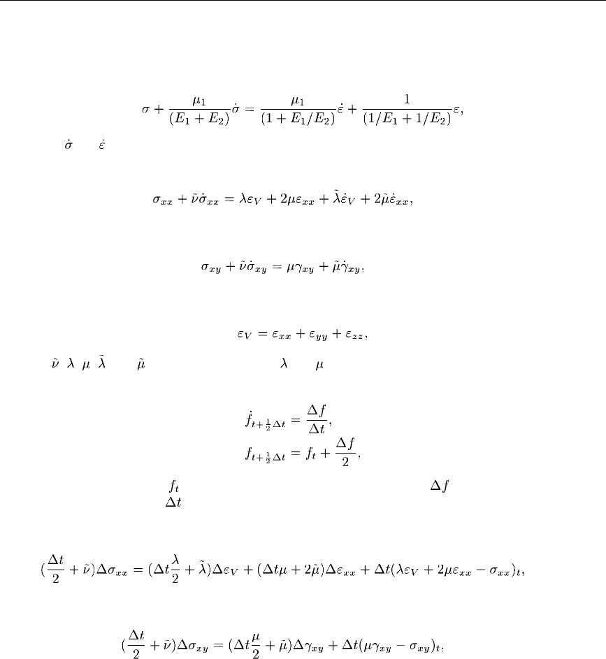
UMAT
Example: Simple linear viscoelastic material
As a simple example of the codin g of user subroutine UMAT, c on sider the linear, viscoelastic model
shown in Figure 1.1.44–1. Althoug h this i s not a very use ful model for real m a terials, it serves to illustrate
how to code the routin e.
The behavior of the one-dimensional model shown in the figure is
where and are the time rates of chan ge of stress and strain. Th is can be generalized for small straining
of an isotropic solid as
etc.,
and
etc.,
where
and , , , ,and are material constants ( and are the Lam é constants).
A simple, stable integration operator for this equation is the central difference operator:
where f is some function, is its value a t the be gin n ing of the increm ent, is the change in the function
over the increm e nt, and
is the time increment.
Applying this to the rate constitutive equations above gives
etc.,
and
etc.,
so that the Jacobian m a trix has the terms
1.1.44–12
Abaqus ID:
Printed on:

UMAT
ε
σ
σ
E
E
2
1
μ
1
Figure 1.1.44–1 Simple linear viscoel a st ic model.
and
The total change in specific energy in an increment for this material is
1.1.44–13
Abaqus ID:
Printed on:

UMAT
whilethechangeinspecific elastic strain energy is
where D is the elastic ity m a trix:
No state variables are needed for this material, so the allocatio n of space fo r them is not necessary.
In a more realistic case a set of parallel models of this type might be used, and the stress com po nents in
each model might be stored as state variables.
For our simple case a user material definition can be used to read in the five constants in the order
, , , ,and so that
The routine can then be coded as follows:
SUBROUTINE UMAT(STRESS,STATEV,DDSDDE,SSE,SPD,SCD,
1 RPL,DDSDDT,DRPLDE,DRPLDT,
2 STRAN,DSTRAN,TIME,DTIME,TEMP,DTEMP,PREDEF,DPRED,CMNAME,
3 NDI,NSHR,NTENS,NSTATV,PROPS,NPROPS,COORDS,DROT,PNEWDT,
4 CELENT,DFGRD0,DFGRD1,NOEL,NPT,LAYER,KSPT,JSTEP,KINC)
C
INCLUDE 'ABA_PARAM.INC'
1.1.44–14
Abaqus ID:
Printed on:
UMAT
C
CHARACTER*80 CMNAME
DIMENSION STRESS(NTENS),STATEV(NSTATV),
1 DDSDDE(NTENS,NTENS),
2 DDSDDT(NTENS),DRPLDE(NTENS),
3 STRAN(NTENS),DSTRAN(NTENS),TIME(2),PREDEF(1),DPRED(1),
4 PROPS(NPROPS),COORDS(3),DROT(3,3),DFGRD0(3,3),DFGRD1(3,3),
5 JSTEP(4)
DIMENSION DSTRES(6),D(3,3)
C
C EVALUATE NEW STRESS TENSOR
C
EV=0.
DEV=0.
DO K1=1,NDI
EV = EV + STRAN(K1)
DEV = DEV + DSTRAN(K1)
END DO
C
TERM1 = .5*DTIME + PROPS(5)
TERM1I = 1./TERM1
TERM2 = (.5*DTIME*PROPS(1)+PROPS(3))*TERM1I*DEV
TERM3 = (DTIME*PROPS(2)+2.*PROPS(4))*TERM1I
C
DO K1=1,NDI
DSTRES(K1) = TERM2+TERM3*DSTRAN(K1)
1 +DTIME*TERM1I*(PROPS(1)*EV
2 +2.*PROPS(2)*STRAN(K1)-STRESS(K1))
STRESS(K1) = STRESS(K1) + DSTRES(K1)
END DO
C
TERM2 = (.5*DTIME*PROPS(2) + PROPS(4))*TERM1I
I1 = NDI
DO K1=1,NSHR
I1 = I1+1
DSTRES(I1) = TERM2*DSTRAN(I1)+
1 DTIME*TERM1I*(PROPS(2)*STRAN(I1)-STRESS(I1))
STRESS(I1) = STRESS(I1)+DSTRES(I1)
END DO
C
C CREATE NEW JACOBIAN
C
1.1.44–15
Abaqus ID:
Printed on:
UMAT
TERM2 = (DTIME*(.5*PROPS(1)+PROPS(2))+PROPS(3)+
1 2.*PROPS(4))*TERM1I
TERM3 = (.5*DTIME*PROPS(1)+PROPS(3))*TERM1I
DO K1=1,NTENS
DO K2=1,NTENS
DDSDDE(K2,K1) = 0.
END DO
END DO
C
DO K1=1,NDI
DDSDDE(K1,K1) = TERM2
END DO
C
DO K1=2,NDI
N2 = K1−1
DO K2=1,N2
DDSDDE(K2,K1) = TERM3
DDSDDE(K1,K2) = TERM3
END DO
END DO
TERM2 = (.5*DTIME*PROPS(2)+PROPS(4))*TERM1I
I1 = NDI
DO K1=1,NSHR
I1 = I1+1
DDSDDE(I1,I1) = TERM2
END DO
C
C TOTAL CHANGE IN SPECIFIC ENERGY
C
TDE=0.
DO K1=1,NTENS
TDE = TDE + (STRESS(K1)-.5*DSTRES(K1))*DSTRAN(K1)
END DO
C
C CHANGE IN SPECIFIC ELASTIC STRAIN ENERGY
C
TERM1 = PROPS(1) + 2.*PROPS(2)
DO K1=1,NDI
D(K1,K1) = TERM1
END DO
DO K1=2,NDI
N2 = K1-1
1.1.44–16
Abaqus ID:
Printed on:
UMAT
DO K2=1,N2
D(K1,K2) = PROPS(1)
D(K2,K1) = PROPS(1)
END DO
END DO
DEE=0.
DO K1=1,NDI
TERM1 = 0.
TERM2 = 0.
DO K2=1,NDI
TERM1 = TERM1 + D(K1,K2)*STRAN(K2)
TERM2 = TERM2 + D(K1,K2)*DSTRAN(K2)
END DO
DEE = DEE + (TERM1+.5*TERM2)*DSTRAN(K1)
END DO
I1 = NDI
DO K1=1,NSHR
I1 = I1+1
DEE = DEE + PROPS(2)*(STRAN(I1)+.5*DSTRAN(I1))*DSTRAN(I1)
END DO
SSE = SSE + DEE
SCD = SCD + TDE − DEE
RETURN
END
1.1.44–17
Abaqus ID:
Printed on:

UMATHT
1.1.45 UMATHT: User subroutine to define a material’s thermal behavior.
Product:
Abaqus/Standard
WARNING : The use of this subroutine generally requires considerable expertise.
You are cautioned that th e implementation of any realistic thermal mod el requires
significant development and testing. Initial testing on models with few elements
under a variety of boundary conditions is strongly recommended.
References
•
“User-defined thermal material behavior,” Section 26.7.2 of the Abaqus Analysis User’s Guide
• *
USER MATERIAL
•
“Freezing of a square solid: the two-dimensional Stefan problem,” Section 1.6.2 of the Abaqus
Benchmarks Guide
•
“UMATHT,” Section 4.1.22 of the Abaqus Verification Guide
Overview
User subroutine UMATHT:
•
can be used to define the thermal constitutive behavior of the material as well as internal heat
generation during heat tran sfer processes;
•
will be called a t all materi al calculation points o f elements for which the material definitio n inclu des
auser-defined t hermal material beh avior;
•
can be used w ith the procedures discussed in “Heat transfer analysis procedures: overview,”
Section 6.5.1 of the Abaqus Analysis User’s Guide;
•
can use solution-depend ent state variables;
•
must define the internal energy per unit mass and its variation with respect to temperature and to
spatial gradients of temperature;
•
must define the heat flux vector and its variation with respect to tem perature and to gradients of
temperature;
•
must upd ate the solutio n-dependent state variables to their values at the en d of the increment;
•
can be used in conjunctionwithusersubroutineUSDFLD to redefine any field variables before they
are passed i n; and
•
is described further in “User-defined thermal material behavior,” Section 26.7.2 of the Abaqus
Analysis User’s Guide.
1.1.45–1
Abaqus ID:
Printed on:

UMATHT
Use of subroutine UMATHT with coupled temperature-displacement and coupled
thermal-electrical-structural elements
User subroutine UMATHT should be used only with reduced-integration o r modified coupled t emperature-
displacement and coupled thermal-electrical-structural elements if the mechanical and thermal fields
are not coupled through plastic dissipation. No such restriction exists with fully integrated coupled
temperature-displacement and coupled thermal-electrical-structural elements.
User subroutine interface
SUBROUTINE UMATHT(U,DUDT,DUDG,FLUX,DFDT,DFDG,
1 STATEV,TEMP,DTEMP,DTEMDX,TIME,DTIME,PREDEF,DPRED,
2 CMNAME,NTGRD,NSTATV,PROPS,NPROPS,COORDS,PNEWDT,
3 NOEL,NPT,LAYER,KSPT,KSTEP,KINC)
C
INCLUDE 'ABA_PARAM.INC'
C
CHARACTER*80 CMNAME
DIMENSION DUDG(NTGRD),FLUX(NTGRD),DFDT(NTGRD),
1 DFDG(NTGRD,NTGRD),STATEV(NSTATV),DTEMDX(NTGRD),
2 TIME(2),PREDEF(1),DPRED(1),PROPS(NPROPS),COORDS(3)
user coding to define U,DUDT,DUDG,FLUX,DFDT,DFDG,
and possibly update STATEV, PNEWDT
RETURN
END
Variables to be defined
U
Internal therm al energy per unit mass, U, at the end of increment. This variab le is passed in as the
value at the start of the increment and must be updated to its value at the end of the increment.
DUDT
Variation of internal thermal energy per unit mass with respect to temperature,
, evaluated at the
end o f the increment.
1.1.45–2
Abaqus ID:
Printed on:
UMATHT
DUDG(NTGRD)
Variation of internal thermal energy per unit m ass with respect to the spatial gradients of temperature,
, at the end of t he increm ent. The size of this array depends on the value of NTGRD as
defined below. This term is typically zero in classical heat transfer analysis.
FLUX(NTGRD)
Heat flux vector,
, at the end of the increment. This variable is passed in with the values at the
beginning of the increment and must be updated to the values at the end of the increment.
DFDT(NTGRD)
Variation of the heat flux vector with respect to temperature,
, evaluated at the end of the
increment.
DFDG(NTGRD,NTGRD)
Variation of the heat flux vector with respect to the spatial gradients of temperature,
,at
the end of the in crem ent. The size of this array depends on the value of NTGRD as defined below.
Variables that can be updated
STATEV(NSTATV)
An array contain ing the solution-dependent state v ariables.
In an uncoupled heat transfer analysis STATEV is passed into UMATHT with the values o f these
variables at the beginning of t he increment. However, any changes in STATEV made in user subrou tine
USDFLD will be included in the values passed into UMATHT,sinceUSDFLD is called before UMATHT.
In addition, if UMATHT is being used in a fully coupled temperature-displacement or coupled thermal-
electrical-structural analysis and user subroutine CREEP, user subroutine UEXPAN, user subrou tine
UMAT, or user subroutine UTRS is used to define the mechanical behav ior of the material, those routines
are called before this routine; therefore, any updating of STATEV done in CREEP, UEXPAN, UMAT,or
UTRS will be included in the values p assed into UMATHT.
In all cases STATEV should be passed back from UMATHT as the values of the state variables at
the end of the current increm ent .
PNEWDT
Ratio of suggested new time increment to the time increment being used (DTIME,seebelow).
This variable allows you to provide input to the automatic time incrementation algori thms in
Abaqus/Standard (if automatic tim e i ncrementation is chosen) .
PNEWDT is set to a large value before each call to UMATHT.
If PNEWDT is redefined to be less than 1.0, A baq us/Stan dard must aban don the time increment
and attempt it again with a smaller time increment. The suggested n ew time increment provided to the
automatic time integration algorithms is PNEWDT × DTIME,wherethePNEWDT used is the minimum
value fo r all calls to user subrou tines that allow redefinition of PNEWDT for this iter a tion.
If PNEWDT is given a value that is greater than 1.0 f or all calls to user subroutines for this iteration
and the increment converges in this iteration, Abaqus/Standard m ay increase the time increment. The
1.1.45–3
Abaqus ID:
Printed on:

UMATHT
suggested new time i ncr ement provided to the automati c time integration algorithms is PNEWDT ×
DTIME,wherethePNEWDT used is the minimum value for all calls to user sub routines for this itera tio n.
If automatic time i ncrementation is not selected in the analysis procedure, values of PNEWDT that
are greater than 1.0 will be ignored and values of PNEWDT that are less than 1.0 will cause the job to
terminate.
Variables passed in for information
TEMP
Temperature at the start of the increm ent.
DTEMP
Increment of tem perature.
DTEMDX(NTGRD)
Current values of the spatial gradients of tem perature,
TIME(1)
Value of step t ime at the begin nin g of the current increment.
TIME(2)
Value of total time at the beginning of the current increment.
DTIME
Time increment.
PREDEF
Array of interpolated values of predefined field variables at this point at the start of the increment, based
on the values read in at the n odes.
DPRED
Array of i ncrements of p redefined field variables.
CMNAME
User-defined m aterial name, left justified.
NTGRD
Number of spatial gradients of temperature.
NSTATV
Number of solution-dependent state variables associated with this material type (defined as described
in “Allocating space” in “User subroutines: overview,” Section 18.1.1 of the Abaqus Analysis User’s
Guide).
PROPS(NPROPS)
User-specified array o f material constants associated with this user m aterial.
1.1.45–4
Abaqus ID:
Printed on:

UMATHT
NPROPS
User-defined number of material c o nstan ts associated with this user material.
COORDS
An array containing the coordinates of this p oin t. These are the current coordinates in a fully coupled
temperature-displacement or coupled thermal-electrical-structural analysis if geometric nonlinearity is
accounted for durin g the step (see “Defining an analysis,” Section 6.1.2 of the Abaqus Analysis User’s
Guide); otherwise, the array contains the origin al coordinates of the point.
NOEL
Element number.
NPT
Integration point number.
LAYER
Layer number (for composite shells and layered solids).
KSPT
Section point number within the c urren t layer.
KSTEP
Step number.
KINC
Increment number.
Example: Using more than one user-defined thermal material model
To use more than one user-defined thermal material model, the variable CMNAME can be tested for
different material names inside user subroutine UMATHT, as illustrated below:
IF (CMNAME(1:4) .EQ. 'MAT1') THEN
CALL UMATHT_MAT1(argument_list)
ELSE IF(CMNAME(1:4) .EQ. 'MAT2') THEN
CALL UMATHT_MAT2(argument_list)
END IF
UMATHT_MAT1 and UMATHT_MAT2 are the actual user material subroutines containing the con st itutive
material models for each material MAT1 and MAT2, respectively. Subroutine UMATHT merely acts as a
directory h ere. The argument list can be the same as th at used in sub ro utine UMATHT.
Example: Uncoupled heat transfer
As a sim ple exam ple of the coding of user subrou tin e UMATHT, consider uncoupled heat transfer analysis
in a material. The equations for this case are developed here, and the corresponding UMATHT is given.
1.1.45–5
Abaqus ID:
Printed on:

UMATHT
This problem can also be solved by specifying thermal conductivity, specific heat, density, and internal
heat generation directly.
First, the equations for an uncoupled heat transfer analysis are outlined.
The basic energy balance is
where V is the volume of solid material with surface area S, i s the density of the material, is the
material time rate of the internal thermal energy, q is the heat flux per unit area of the body flowing into
the body, and r is the heat sup p li ed extern ally in to the body per unit volume.
A heat flux vector
is defined such that
where is the unit outward normal to th e surface S. Introducing the above relation into the energy balance
equation and using the d ivergence theorem, the following relation is obtained:
The corresponding weak fo rm is given by
where
is the temperature gradient and is an arbitrary variational field s atisfy ing the essen tial boundary
conditions.
Introducing the backward difference integration algorithm:
the weak form of the energy balance equation becomes
This nonlinear system is solved using Newton’s m etho d.
In the above equations the thermal constitutive behavior o f the material is given by
1.1.45–6
Abaqus ID:
Printed on:

UMATHT
and
where are state variables.
The Jacobian for Newton’s method is given by (after dropping the subscrip ts
on U)
The thermal constitutive behavior for this example is now defined. We assume a constant specific
heat for the material. T he heat conduction in the m aterial is assumed to be gov ern ed by Fourier’s law.
The internal thermal energy per unit mass is defined as
with
where c is the specific heat of the material and
Fourier’s law for heat conduction is given as
where is the therm al conduct ivi ty mat rix and is position, so that
and
The assumption of conductivity without any temperatu re dependence implies that
1.1.45–7
Abaqus ID:
Printed on:

UMATHT
No state variables are needed for this material, so the allocatio n of space fo r them is not necessary.
A thermal user material definition can be used to read in the two constants for our simple case,
namely the specific heat, c,andthecoefficient of thermal cond uctivity, k,sothat
SUBROUTINE UMATHT(U,DUDT,DUDG,FLUX,DFDT,DFDG,
1 STATEV,TEMP,DTEMP,DTEMDX,TIME,DTIME,PREDEF,DPRED,
2 CMNAME,NTGRD,NSTATV,PROPS,NPROPS,COORDS,PNEWDT,
3 NOEL,NPT,LAYER,KSPT,KSTEP,KINC)
C
INCLUDE 'ABA_PARAM.INC'
C
CHARACTER*80 CMNAME
DIMENSION DUDG(NTGRD),FLUX(NTGRD),DFDT(NTGRD),
1 DFDG(NTGRD,NTGRD),STATEV(NSTATV),DTEMDX(NTGRD),
2 TIME(2),PREDEF(1),DPRED(1),PROPS(NPROPS),COORDS(3)
C
COND = PROPS(1)
SPECHT = PROPS(2)
C
DUDT = SPECHT
DU = DUDT*DTEMP
U = U+DU
C
DO I=1, NTGRD
FLUX(I) = −COND*DTEMDX(I)
DFDG(I,I) = −COND
END DO
C
RETURN
END
1.1.45–8
Abaqus ID:
Printed on:

UMESHMOTION
1.1.46 UMESHMOTION: User subroutine to specify mesh motion constraints during
adaptive meshing.
Product:
Abaqus/Standard
References
•
“Defining ALE ad aptive mesh domains in Abaqus /Stand ard,” Section 12.2.6 of the Abaq us Analysis
User’s Guide
• *
ADAPTIVE MESH
• *
ADAPTIVE MESH CONSTRAINT
Overview
User subro utine UMESHMOTION:
•
is called at the end of any increment where adaptive m eshing is perform ed (as specified by the
frequencyinincrements);
•
can be used to define the motion of nodes in an adaptive m esh constraint node set; and
•
can call utility routines GETVRN, GETNODETOELEMCONN,andGETVRMAVGATNODE to access
results data at the node.
Accessing node point data
You are provided with access to the values of the node point quantities at the end of the i ncrem ent
through the utili ty rou tine GETVRN descr ib e d in “Obtaining node point informat ion ,” Section 2.1.9.
You can also access v alues of material point quantities extrapolated to, and averaged, at nodes at the
end of the increment through the utility routine GETVRMAVGATNODE describedin“Obtainingmaterial
point information averaged at a node,” Section 2.1.8. GETVRMAVGATNODE req uir es the list of e l ements
attached to the node, which is obtai ned by call ing th e u til ity r out ine GETNODETOELEMCONN described
in “Obtaining node to element c onnectivity,” Sect ion 2.1.10.
User subroutine interface
SUBROUTINE UMESHMOTION(UREF,ULOCAL,NODE,NNDOF,
* LNODETYPE,ALOCAL,NDIM,TIME,DTIME,PNEWDT,
* KSTEP,KINC,KMESHSWEEP,JMATYP,JGVBLOCK,LSMOOTH)
C
INCLUDE 'ABA_PARAM.INC'
C
DIMENSION ULOCAL(NDIM),JELEMLIST(*)
DIMENSION ALOCAL(NDIM,*),TIME(2)
1.1.46–1
Abaqus ID:
Printed on:

UMESHMOTION
DIMENSION JMATYP(*),JGVBLOCK(*)
C
user coding to define ULOCAL
and, optio nally PNEWDT
RETURN
END
Variable to be defined
ULOCAL
Components of the mesh displacement or velocity of the adaptive mesh constraint node, described in
the coordinate system ALOCAL. ULOCAL will be passed into the routine as values determined by the
mesh smoothing algorithm. All components of the mesh displacement or velocity will be applied; i.e.,
you do not have the ability to select the directions in which t he mesh displacement should be applied.
Variables that can be updated
PNEWDT
Ratio of suggested n ew time increment to the time increment currently bein g used (DTIME,see
below). This variable allows you to provide input to the automatic tim e increm ent a tion algorithms in
Abaqus/Standard (if automatic tim e i ncrementation is chosen) .
PNEWDT is set to a large value before each call to UMESHMOTION.
The suggested new time increment provided to the aut omatic time integrati on algorithm s is
PNEWDT × DTIME,wherethePNEWDT used is the minimum valu e for all calls to user subroutines
that allow redefi nition of PNEWDT for this increment.
If automatic time increme ntat ion is not selected in the analysis procedure, values of PNEWDT
greater than 1.0 w ill be ignored and values of PNEWDT less than 1.0 will cause the job to terminat e.
LSMOOTH
Flag specifying that surface smoothing be applied after application of the me sh m oti on constraint. Set
LSMOOTH to 1 to enable surface smoothing. When t his flag is set, the constraint defined in ULOCAL
will be modified by the smoothing algorithm. In cases where ULOCAL describes m esh motion normal
to a surface, the smoothing will have a minor impact on this normal component of mesh motion.
Variables passed in for information
UREF
The v alue of the user-specified displacement or velocity provided as part of the adaptive mesh constraint
definition. This value is updated b ased on any a m plitude definitions used with the adaptive mesh
constraint or default ramp amplitude variations associated with the current step.
1.1.46–2
Abaqus ID:
Printed on:
UMESHMOTION
NODE
Node number.
NNDOF
Number of degrees of freedom at the node.
LNODETYPE
Node type flag.
LNODETYPE=1 indicates that the node is on the interior of the adaptive mesh r egion.
LNODETYPE=2 indicates that the node is involved in a tied constraint.
LNODETYPE=3 indicates that the node is at the corner of the boundary of an adaptive m esh region.
LNODETYPE=4 indicates that the node lies on the edge of a boundary o f a n adaptive mesh regio n.
LNODETYPE=5 indicates that the node lies on a flat surface on a boundary of the adaptive mesh
region.
LNODETYPE=6 indicates that the node participates in a constraint (other than a tied constraint)
as a master node.
LNODETYPE=7 indicates that the node participates in a constraint (other than a tied constraint)
as a slave node.
LNODETYPE=10 indicates that a concentrated load is applied to the node.
ALOCAL
Local coordinate system aligned with the tangent to the adaptive mesh domain at the node. If the node
is on the interior of the adaptive m esh dom ain, ALOCAL will be set to the identity matrix. In other
cases the 1-direction is along an edge or in the plane of a flat surface. When NDIM=2, the 2-direction
is normal to the surface. When NDIM=3, the 2-direction also lies in the plane of a fl at surface or is
arbitrary if the node is o n an edge. When NDIM=3 the 3-direction is normal to the surface or is arbitrary
if the node is on an edge.
NDIM
Number o f coordinate dimensions.
TIME(1)
Current value of step time.
TIME(2)
Current value of total time.
DTIME
Time increment.
KSTEP
Step number.
KINC
Increment number.
1.1.46–3
Abaqus ID:
Printed on:
UMESHMOTION
KMESHSWEEP
Mesh sweep num ber.
JMATYP
Variable that must be passed into the GETVRMAVGATNODE utility routine to access local results at the
node.
JGVBLOCK
Variable that must be passed into the GETVRN, GETNODETOELEMCONN,andGETVRMAVGATNODE
utility routines to access local results at the node.
1.1.46–4
Abaqus ID:
Printed on:

UMOTION
1.1.47 UMOTION: User subroutine to specify motions during cavity radiation heat transfer
analysis or steady-state transport analysis.
Product:
Abaqus/Standard
References
•
“Cavity radiation,” Section 41.1.1 of the Abaqus Analysis User’s Guide
•
“Steady-state transport analysis,” Section 6.4.1 of the Abaqus Analysis User’s Guide
• *
MOTION
• *
TRANSPORT VELOCITY
Overview
User subroutine UMOTION:
•
can be used either to define the magnitude of the translatio nal motion for degrees of freedom
specified as a predefined field in a cavity radiation heat transfer analysis or to define the magni tude
of the rotational velocity in a steady-state transport step; and
•
will overwrite any mo tio n or transpor t velocity magnitudes if they are defined directly (and possibly
modified by including an am plitude reference) outside the user subroutine.
User subroutine interface
SUBROUTINE UMOTION(U,KSTEP,KINC,TIME,NODE,JDOF)
C
INCLUDE 'ABA_PARAM.INC'
C
DIMENSION U,TIME(2)
C
user coding to define U
RETURN
END
1.1.47–1
Abaqus ID:
Printed on:

UMOTION
Variable to be defined
U
Total value of the compo nent o f the translation due to prescribed motion for the degree of freedom
specified by JDOF. U will be passed into the routine as the value defined by any magnitude an d/or
amplitude specification in the m otion definitio n for the degree of freedom JDOF. The total value of
the translation must be given in user subroutine UMOTION, regardless of the type of motion de fined
(displacement or v elocity).
When used in conjunction with a steady-state transport analysis, U defines the magnitude of the
rotational velo city. In such a case JDOF is passed in as 0.
Variables passed in for information
KSTEP
Step number.
KINC
Increment number.
TIME(1)
Current value of step time.
TIME(2)
Current value of total time.
NODE
Node number.
JDOF
Degree of freedom. When used in a steady-state transport analysis, JDOF is passed in as 0.
1.1.47–2
Abaqus ID:
Printed on:

UMULLINS
1.1.48 UMULLINS: User subroutine to define damage variable for the Mullins effect
material model.
Product:
Abaqus/Standard
References
•
“Mullins effect,” Section 22.6.1 of the Abaqus Analysis User’s Guide
• *
MULLINS EFFECT
•
“Mullins effect and permanent set,” Section 2.2.3 of the Abaqus Verification Guide
Overview
User subrou tine UMULLINS:
•
can be used to definethedamagevariablefortheMullinseffect material model, including the use
of the Mul lins effect approach to model energy dissip a tio n in elastomeric foams;
•
will be called a t all materi al calculation points o f elements for which the material defini tion contains
auser-defi ned Mullin s effect; and
•
should be used when you do not w ant to use the Ogden and Roxburgh form of the damage v ariab le,
, that is used by Abaqus/Standard.
User subroutine interface
SUBROUTINE UMULLINS(NUMPROPS,PROPS,UMAXNEW,UMAXOLD,SEDDEV,
1 ETA,DETADW,DMGDISSOLD,DMGDISSNEW,SENERNEW,NUMSTATEV,STATEV,
2 TEMP,DTEMP,NUMFIELDV,FIELDV,FIELDVINC,CMNAME,LINPER)
C
INCLUDE 'ABA_PARAM.INC'
C
CHARACTER*80 CMNAME
DIMENSION PROPS(*),STATEV(*),FIELDV(*),FIELDVINC(*)
user coding to define ETA, DETADW,
and, optio nally, DMGDISSNEW, SENERNEW, STATEV
RETURN
END
1.1.48–1
Abaqus ID:
Printed on:

UMULLINS
Variables to be defined
ETA
The damage variable,
.
DETADW
The derivative of the damage variable with respect to the elastic strain energy density of the undamaged
material,
. This quantity is needed for the Jacobian of the o verall system of equations and needs to
be defined accurately to ensure good convergence characteristics.
Variables that can be updated
DMGDISSNEW
The energy dissipation density at the end of the increment. This q uantity can be de fined either in total
form or in an incremental manner using the old value of the da mag e dissipation DMGDISSOLD and the
increment in dam age dissipatio n. This quantity is used for output purposes only.
SENERNEW
The recoverable strain energy d ensity at the end o f the incremen t. This quantity is u sed for output
purposes only.
STATEV
Array co ntai ning the user-defined solution-dependent s tate variables at t his point. These are supplied a s
values at the start of the increment or as values updated by other user subroutines (see “User subroutines:
overview,” Section 18.1.1 of the Abaqus Analysis User’s Guide) and must be returned as values at the
end o f the increment.
Variables passed in for information
UMAXNEW
The value, at the end of the increment, of the maxim um primary strain energy density over its entire
deformation h istory.
UMAXOLD
The value, at the beginning of the increment, of the maxim um primary strain e nergy density over its
entire deformation history.
SEDDEV
The value, at t he end of the increm ent, of the deviatoric primary strain energy d e nsity wh en the prima ry
material behavior is hyperelastic. The value, at the end of the increment, of the total primary strain
energy density when the primary material behavior is hyperfoam.
DMGDISSOLD
The value of energy dissipated at the beginning of the increment.
1.1.48–2
Abaqus ID:
Printed on:
UMULLINS
CMNAME
User-specified material name, left justified.
NUMSTATEV
Number of soluti on- depen dent state variables associated with this material (defined as described in
“Allocating space” in “User subroutines: overview,” S ection 18.1.1 of the Abaqus A nalysis User’s
Guide).
NUMPROPS
Number of material properties entered for this user-defined hyperelastic material.
PROPS
Array of material properties entered for this user-defined hyperelastic material.
TEMP
Temperature at the start of the increm ent.
DTEMP
Increment of tem perature.
NUMFIELDV
Number of field variables.
FIELDV
Array o f interpolated values of predefined field variables at this material point at the beginning of the
increment based on the values read in at the nodes (initial values at the beginning o f th e an alysis and
current values during the analysis).
FIELDVINC
Array of increments of predefined field variables at this material point for this increm e nt; this includes
any values u pdated by user subroutine USDFLD.
LINPER
Linear perturbation flag. LINPER=1 if the step is a l inear perturbation step. LINPER=0 if the step is
a general step.
1.1.48–3
Abaqus ID:
Printed on:

UPOREP
1.1.49 UPOREP: User subroutine to define initial fluid pore pressure.
Product:
Abaqus/Standard
References
•
“Initial conditions in Ab aqu s /S tandard and Abaqus/Explicit ,” Section 34.2.1 of the Abaqus Analysis
User’s Guide
•
“Coupled pore fluid diffusion and s tr ess analysis,” Section 6.8.1 of the Abaq us An a lysi s User’s
Guide
• *
INITIAL CONDITIONS
Overview
User subroutine UPOREP:
•
allows for the specification o f the initial pore pressure values of a porous medium;
•
can be used to define initial pore pressure values as functio ns o f nod al coordin ates an d/o r nod e
numbers; and
•
will be called to define initial fluid pore pressure values at all nodes of a coupled pore fluid diffusion
and stress analysis whenever user-defined initial pore pressure conditions are specified.
User subroutine interface
SUBROUTINE UPOREP(UW0,COORDS,NODE)
C
INCLUDE 'ABA_PARAM.INC'
C
DIMENSION COORDS(3)
C
user coding to define UW0
RETURN
END
Variable to be defined
UW0
Initial fluid pore pressure.
1.1.49–1
Abaqus ID:
Printed on:

UPOREP
Variables passed in for information
COORDS
An array containing the current coordinates of this node.
NODE
Node number.
1.1.49–2
Abaqus ID:
Printed on:

UPRESS
1.1.50 UPRESS: User subroutine to specify prescribed equivalent pressure stress
conditions.
Product:
Abaqus/Standard
References
•
“Mass diffusion analysis,” Section 6.9.1 of the Abaqus Analysis User’s Guide
• *
PRESSURE STRESS
•
“UTEMP, UFIELD, UMASFL,andUPRESS,” Section 4.1.25 of the Ab aqus Verificatio n Guide
Overview
User subroutine UPRESS:
•
allows you to prescribe equivalen t pressure stress values at the nodes of a model;
•
will be called in a mass d iffusion analysis whenever a cu rrent value of equivalent pressure stress is
needed for a node that has user-defined pressure stress conditions;
•
can be used to modify any pressure stresses read in from a results file; and
•
ignores any equivalent pressure stresses provided for the associated pressure stress definitio n outside
the user subrouti ne.
User subroutine interface
SUBROUTINE UPRESS(PRESS,KSTEP,KINC,TIME,NODE,COORDS)
C
INCLUDE 'ABA_PARAM.INC'
C
DIMENSION TIME(2), COORDS(3)
C
user coding to define PRESS
RETURN
END
Variable to be defined
PRESS
Total value of the equivalen t p ressure stress at the node.
1.1.50–1
Abaqus ID:
Printed on:

UPRESS
You may have also requested equivalent pressure stress to be set in one of two other ways: from
a previously generated results file or via d irect data input. When PRESS is passed into user subroutine
UPRESS, it will contain equivalent pressure stresses obtained from the results file only. You can modify
these values within this routine. Any values given as direct data input will be ignored.
Variables passed in for information
KSTEP
Step number.
KINC
Increment number.
TIME(1)
Current value of step time.
TIME(2)
Current value of total time.
NODE
Node number.
COORDS
An array containing the coordinates of this node.
1.1.50–2
Abaqus ID:
Printed on:

UPSD
1.1.51 UPSD: User subroutine to define the frequency dependence for random response
loading.
Product:
Abaqus/Standard
References
•
“Random response analysis,” Section 6.3.11 of the Abaqus An alysis User’s Guide
• *
RANDOM RESPONSE
• *
PSD-DEFINITION
•
“Random respon se to jet noise excitation,” Section 1.4.10 of the Abaqus Benchmarks Guide
Overview
User subroutine UPSD:
•
will be called once for each frequency at which calculations will be made during a random response
analysis if the frequency function is defined in a user subroutine;
•
is used to define complicated frequency dependencies for the cross-spectral density matrix of the
random loading; and
•
ignores any data given for the associated frequency function outside the user subroutine.
User subroutine interface
SUBROUTINE UPSD(PSD,PSDR,PSDI,FREQ,KSTEP)
C
INCLUDE 'ABA_PARAM.INC'
C
CHARACTER*80 PSD
user coding to define PSDR and PSDI
RETURN
END
Variables to be defined
PSDR
Real part of the frequency function at this frequency.
1.1.51–1
Abaqus ID:
Printed on:

UPSD
PSDI
Imaginary part of the frequency function at this frequency.
Variables passed in for information
PSD
User-specified name for this frequency function definition, left justified.
FREQ
Frequency, in radians per time.
KSTEP
Step number.
1.1.51–2
Abaqus ID:
Printed on:

URDFIL
1.1.52 URDFIL: User subroutine to read the results file.
Product:
Abaqus/Standard
References
•
“Results file output form at,” Section 5.1.2 of the Abaqus Analysis User’s Gu ide
•
“Accessing the results file information,” Section 5.1.3 of the Abaq us Analysis User’s Guide
•
“Utility routines for accessing the results file,” Section 5.1.4 of the Abaqus Analysis User’s G uid e
Overview
User subroutine URDFIL:
•
can be used to access the results fileduringananalysis;
•
is called at th e end o f any incr ement in which new inform ation is written to the results file;
•
must call the utility routine DBFILE to read records from the results file (see “Utility routines for
accessing the results file,” Section 5.1.4 of the Abaqus Analysis User’s Guide);
•
can call the utility routine POSFIL to read fro m the results file starting at a specified step and
increment as opposed to the beginning of the file, which would otherwise be done (see “Utility
routines for accessing the results file,” Section 5.1.4 of the Abaqus Analysis User’s Guide);
•
can force an analysis to terminate upon completion of a call by means of the variable LSTOP;
•
allows the last increment written to the results file to be overwritten by means of the variable
LOVRWRT;and
•
allows access to the complete results file in a restarted job if the new result s file is being appended
to th e old resu lts file (s ee the descrip tion of the executio n option fil in “Abaqus/Standard,
Abaqus/Explicit, and Abaqus/CFD execution,” Section 3.2.2 of th e A b aqus An alysis User’s
Guide).
User subroutine interface
SUBROUTINE URDFIL(LSTOP,LOVRWRT,KSTEP,KINC,DTIME,TIME)
C
INCLUDE 'ABA_PARAM.INC'
C
DIMENSION ARRAY(513),JRRAY(NPRECD,513),TIME(2)
EQUIVALENCE (ARRAY(1),JRRAY(1,1))
user coding to read the results file
RETURN
END
1.1.52–1
Abaqus ID:
Printed on:

URDFIL
Variables to be defined
In all cases
LSTOP
Flag to indicate whether an analysis should continue. The analysis will be terminated if LSTOP is set
to 1. Otherwise, the analy sis will con tin ue.
LOVRWRT
Flag to indicate that the info rmation written to the results file for the increment can be overwritten. If
LOVRWRT is set to 1, information for the current increm ent will be over wri tten by i nformation written
to the results file in a subsequent increment unless the current increment is the final increment written to
the results file. The purpose of this flag is to reduce the size of the results file by allowing information
for an incremen t to be overwritten by information for a subsequent increment.
DTIME
Time increment. This variable allows you t o provide input to the automatic time inc rementation
algorithms in Abaqus (if automatic time incrementation is chosen). It is passed in as the value of
the next time incremen t to be taken and can be updated to increase or reduce the time increment. If
automatic time incrementation is not selected in the analysis procedure, updated values of DTIME are
ignored.
Only if utility routine POSFIL is called
NSTEP
Desired step at which file reading will begin via utility ro u ti ne DBFILE.IfNSTEP is set to 0, the first
available step will be read.
NINC
Desired increment at which file reading will begin via utility routine DBFILE.IfNINC is set to 0, the
first available increment of the specified step will be read.
Variables passed in for information
KSTEP
Step number.
KINC
Increment number.
TIME(1)
Value of the step ti me at the end of t he increment.
TIME(2)
Value of the total time at the end of the incr emen t.
1.1.52–2
Abaqus ID:
Printed on:

URDFIL
Example: Terminating an analysis upon exceeding a Mises stress limit
The example below reads the values of Mises stress for the current increm ent from record 12 in the results
file and terminates the analysis if any of the values of Mises stress written to the results file exceed 2.09
×10
8
. H ere, POSFIL is used to position you to read from the current increment.
SUBROUTINE URDFIL(LSTOP,LOVRWRT,KSTEP,KINC,DTIME,TIME)
C
INCLUDE 'ABA_PARAM.INC'
C
DIMENSION ARRAY(513),JRRAY(NPRECD,513),TIME(2)
EQUIVALENCE (ARRAY(1),JRRAY(1,1))
PARAMETER(TOL=2.09D8)
C
C FIND CURRENT INCREMENT.
C
CALL POSFIL(KSTEP,KINC,ARRAY,JRCD)
DO K1=1,999999
CALL DBFILE(0,ARRAY,JRCD)
IF (JRCD .NE. 0) GO TO 110
KEY=JRRAY(1,2)
C
C RECORD 12 CONTAINS VALUES FOR SINV
C
IF (KEY.EQ.12) THEN
IF (ARRAY(3).GT.TOL) THEN
LSTOP=1
GO TO 110
END IF
END IF
END DO
110 CONTINUE
C
RETURN
END
Example: Terminating an analysis when the maximum Mises stress value stops increasing
This example demonstrates the use of URDFIL and POSFIL to stop an analysis when the maximum
value o f Mises stress in the m odel does not i ncrease from one increment in the results file to the next.
A data statement is used to save the maximum M i ses stress value from the last increment. LOVRWRT is
also used in this case to overwrite an increment in the results file once it has been read in URDFIL.
1.1.52–3
Abaqus ID:
Printed on:
URDFIL
The subroutine shown below must be modified to define the maximum Mises stress in the data
statement each time a job is restarted. This can be avoided by removing the LOVRWRT=1 statem ent
and recoding the r outine to read both the previous and the current increment to check that the Mises
stress increases from one increment to the next (in this case you must correctly handle the first increme nt
written to the results file as there will be no previous increment). The results file must also be properly
appended on restart if you wish to com pare the values of Mises stress between the first increm ent of a
restart and the final increment of the job being restarted. T his approach has the disadvantage that th e
results file may become quite large, as no information in the file will be overwr it ten.
SUBROUTINE URDFIL(LSTOP,LOVRWRT,KSTEP,KINC,DTIME,TIME)
C
INCLUDE 'ABA_PARAM.INC'
C
DIMENSION ARRAY(513),JRRAY(NPRECD,513),TIME(2)
EQUIVALENCE (ARRAY(1),JRRAY(1,1))
C
C INITIALIZE THE OLD MAXIMUM. FOR A JOB THAT IS BEING RESTARTED
C THIS VALUE SHOULD BE SET TO THE MAXIMUM MISES STRESS IN THE
C ORIGINAL ANALYSIS.
C
DATA OLDMAX/-1.D0/
C
CURRMAX = 0.D0
C
C FIND CURRENT INCREMENT.
C
CALL POSFIL(KSTEP,KINC,ARRAY,JRCD)
C
C SEARCH FOR THE HIGHEST VALUE OF MISES STRESS
C AND STORE THIS IN CURRMAX
C
DO K1=1,999999
CALL DBFILE(0,ARRAY,JRCD)
IF (JRCD.NE.0) GO TO 110
KEY=JRRAY(1,2)
IF (KEY.EQ.12) THEN
IF (ARRAY(3).GT.CURRMAX) CURRMAX=ARRAY(3)
END IF
END DO
110 CONTINUE
C
C COMPLETED READING OF CURRENT INCREMENT. NOW CHECK TO
C SEE IF VALUE OF MISES STRESS HAS INCREASED SINCE
1.1.52–4
Abaqus ID:
Printed on:
URDFIL
C LAST INCREMENT
C
IF (CURRMAX.LE.OLDMAX) LSTOP=1
OLDMAX=CURRMAX
LOVRWRT=1
C
RETURN
END
1.1.52–5
Abaqus ID:
Printed on:

USDFLD
1.1.53 USDFLD: User subroutine to redefine field variables at a material point.
Product:
Abaqus/Standard
References
•
“Obtaining material point information in an Abaqus/Standard analysis,” Section 2.1.6
•
“Material data definitio n,” Section 21.1.2 o f the Abaqus Analysis User’s Guide
• *
USER DEFINED FIELD
•
“Damage and failure of a laminated com po site plate,” Section 1.1.14 of the Abaqus Example
Problems Guide
•
“USDFLD,” Section 4.1.24 of the Abaqus Verification Guide
Overview
User subroutine USDFLD:
•
allowsyoutodefine field variables at a material point as functions of time or of any of the available
material point quantities lis ted in the O utput Variable Identifiers table (“Abaq us/Stand ard output
variable identifiers,” Section 4.2.1 of the Abaqus Analysis User’s Guide) e xcept the user-de fined
output variables UVA RM and UVA RM n;
•
can be used to introduce solution-dependent m aterial properties since such properties can easily b e
defined as functions of field variables;
•
will be called at all material points of elements for w hich the material definition includes user-
defined field variables;
•
must call utility routine GETVRM to access material point data;
•
can use and up date state variables; and
•
can be used in conjunction with user subroutine UFIELD to prescribe prede fined field variables.
Explicit solution dependence
Since this routine provides access to material point quantities only at the start of the increment, the
solution dependence introduced in this way is explicit: the material properties for a given increment are
not influenced by the results obtained during the increment. Hence, the accuracy of the results depends
on the size of the time increment. Therefore, you can control the time increm entinthisroutinebymeans
of the variable PNEWDT.
Defining field variables
Before user subroutine USDFLD is called, the values of the field variables at the material point are
calculated by interpolation from the values defined at the nodes. Any chang es to the field variables
in the user subroutine are local to the material point: the nodal field variables retain the values defined
1.1.53–1
Abaqus ID:
Printed on:

USDFLD
as initial co ndi tions, pre defined field variables, or in u ser subroutine UFIELD. The values of the field
variables defined in this routine are us ed to calculate values of m aterial properties that are defined to
depend on field variables and are passed into other user subroutines that are called at the material point,
such as the follow ing:
•
CREEP
•
HETVAL
•
UEXPAN
•
UHARD
•
UHYPEL
•
UMAT
•
UMATHT
•
UTRS
Output of the user-defined field variables at the m aterial points can be obtained with the element
integration p oint outp ut variab le FV (see “Abaqus/Standard output variable identifiers,” Section 4.2.1
of the Abaqus Analysis User’s Guide).
Accessing material point data
You are provided with access t o the values of the material point quantities at the start of the increment (or
in the base state in a linear perturbation step) through the utility routi n e GETVRM described in “Obtaining
material point in fo rm a tion in an Abaqus/ St andard analysis,” Section 2.1.6. The values of the material
point quantities are obtained by calling GETVRM with the appropriate output variable keys. The values
of the material point data are recovered in the arrays ARRAY, JARRAY,andFLGRAY fo r floating point,
integer, and character data, respectively. You may not get values of some mater ial p oin t quantities that
have not been defined at t he start of the increment; e.g., ER.
State variables
Since the redefinition of field variables in USDFLD is local to the current increment (field variables are
restored to the values interpolated from the nodal values at the start o f each increm ent), any history
dependence required to update material properties by using this subroutin e must be introduced with user-
defined state variables.
The state variables can be updated in USDFLD and then passed into other user subroutines that can
be called at this material point, such as t hose listed abov e. Yo u specify the number of such state variables,
as show n in the example at the end of this section (see also “Allocating space” in “User subroutines:
overview,” Section 18.1.1 of the Abaqus Analysis User’s Guide).
User subroutine interface
SUBROUTINE USDFLD(FIELD,STATEV,PNEWDT,DIRECT,T,CELENT,
1 TIME,DTIME,CMNAME,ORNAME,NFIELD,NSTATV,NOEL,NPT,LAYER,
1.1.53–2
Abaqus ID:
Printed on:

USDFLD
2 KSPT,KSTEP,KINC,NDI,NSHR,COORD,JMAC,JMATYP,MATLAYO,LACCFLA)
C
INCLUDE 'ABA_PARAM.INC'
C
CHARACTER*80 CMNAME,ORNAME
CHARACTER*3 FLGRAY(15)
DIMENSION FIELD(NFIELD),STATEV(NSTATV),DIRECT(3,3),
1 T(3,3),TIME(2)
DIMENSION ARRAY(15),JARRAY(15),JMAC(*),JMATYP(*),COORD(*)
user coding to define FIELD and, if necessary, STATEV and PNEWDT
RETURN
END
Variable to be defined
FIELD(NFIELD)
An array containing the field variables at the current material point. These are passed in with the values
interpolated from the nodes at the end of the current increment, as specified with initial c ondition
definitions, predefined field variable definitions, or user subroutine UFIELD. The interpolation is
performed using the same scheme used to interpolate t emperatures: an average value is used for linear
elements; an approximate l inear variation is used for quadratic elements (also see “Solid (continuum)
elements,” Section 28.1.1 of the Abaqus Analysis User’s Guide). The updated values are used to
calculate the values of material properties that are defined to depend on field variables and are passed
intootherusersubroutines(CREEP, HETVAL, UEXPAN, UHARD, UHYPEL, UMAT, UMATHT,and
UTRS) that are called at this material p oint.
Variables that can be updated
STATEV(NSTATV)
An array containing the solution-dependent s tate variables. These are passed in as the values at the
beginning of the i ncrement. In all cases STATEV can be updated in this subro utine, and the updated
values are passed into o ther user subroutines (CREEP, HETVAL, UEXPAN, UMAT, UMATHT,andUTRS)
that are called at this material point. The number of state variables associated with this material point
is defined as described in “Allocating space” in “User subroutines: overview,” Section 18.1.1 of the
Abaqus Analysis User’s Guide.
PNEWDT
Ratio of suggested new time increment to the time increment being used (DTIME,seebelow).
This variable allows you to provide input to the automatic time incrementation algori thms in
Abaqus/Standard (if automatic tim e i ncrementation is chosen) .
1.1.53–3
Abaqus ID:
Printed on:

USDFLD
PNEWDT is set to a large value before each call to USDFLD.
If PNEWDT is redefined to be less than 1.0, A baq us/Stan dard must aban don the time increment
and attempt it again with a smaller time increment. The suggested n ew time increment provided to the
automatic time integration algorithms is PNEWDT × DTIME,wherethePNEWDT used is the minimum
value fo r all calls to user subrou tines that allow redefinition of PNEWDT for this iter a tion.
If PNEWDT is given a value that is greater than 1.0 f or all calls to user subroutines for this iteration
and the increment converges in this iteration, Abaqus/Standard m ay increase the time increment. The
suggested new time i ncr ement provided to the automati c time integration algorithms is PNEWDT ×
DTIME,wherethePNEWDT used is the minimum value for all calls to user sub routines for this itera tio n.
If automatic time i ncrementation is not selected in the analysis procedure, values of PNEWDT that
are greater than 1.0 will be ignored and values of PNEWDT that are less than 1.0 will cause the job to
terminate.
Variables passed in for information
DIRECT(3,3)
An array containing the direction cosines of the material directions in terms of the global b
asis
directions. DIRECT(1,1), DIRECT(2,1), DIRECT(3,1) give the (1, 2, 3) components of the
first material direction; DIRECT(1,2), DIRECT(2,2), DIRECT(3,2) give the second material
direction, etc. For shell and membrane elem ents, the first two directions are in the plane of the element
and the third direction is the normal. This information is not availab le for beam element s .
T(3,3)
An array containing the direction cosines of the material orientation components relative to the element
basis directions. This is the orien tation that defines the material directions (DIRECT)intermsof
the element basis directions. For continuum elements T and DIRECT are identical. For shell and
membrane elements T(1,1)
, T(1,2) , T(2,1) , T(2,2) ,
T(3,3)
, and all other components are zero, where is the counterclockwise rotation around the
normal vector that defines the orientation. If no orientatio n is used, T is an identity m at ri x. Ori e ntat ion
is not available for beam elements.
CELENT
Characteristic element length. This is a typical length of a line across an element for a fi rst-order
element; it is half of the same typical length for a second-order element. For beams and trusses it is a
characteristic length along the element axis. For membranes and shells it is a characteristic length in
the reference surface. For axisymmetric elements it is a characteristic length in the
plane only.
TIME(1)
Value of step t ime at the begin nin g of the current increment.
TIME(2)
Value of total time at the beginning of the current increment.
1.1.53–4
Abaqus ID:
Printed on:
USDFLD
DTIME
Time increment.
CMNAME
User-specified material name, left justified.
ORNAME
User-specified local orientation nam e, left justified.
NFIELD
Number of field variables defined at th is m aterial point.
NSTATV
User-defined number of solution-dependent state variables (see “Allocating space” in “User
subroutines: overview,” Section 18.1.1 of the Abaqus Analysis User’s Guide).
NOEL
Element number.
NPT
Integration point number.
LAYER
Layer number (for composite shells and layered solids).
KSPT
Section point number within the c urren t layer.
KSTEP
Step number.
KINC
Increment number.
NDI
Number of direct stress components at this point.
NSHR
Number of shear stress components at this point.
COORD
Coordinates at this material point.
JMAC
Variable that must be passed into the GETVRM utility routine to access an output variable.
1.1.53–5
Abaqus ID:
Printed on:

USDFLD
JMATYP
Variable that must be passed into the GETVRM utility routine to access an output variable.
MATLAYO
Variable that must be passed into the GETVRM utility routine to access an output variable.
LACCFLA
Variable that must be passed into the GETVRM utility routine to access an output variable.
Example: Damaged elasticity model
Included below is an example of user su bro utine USDFLD. In this example a truss element is loaded
in tension. A damaged elasticity model is introduced: the modulus decreases as a function of the
maximum tensile strain that occurred during the loading history. The maximum tensile strain is s tored
as a solution-dependent state variable—see “Defining solution-dependent field variables” in “Predefined
fields,” Section 34.6.1 of the Abaqus Analysis User’s G uide.
Input file
*
HEADING
DAMAGED ELASTICITY MODEL WITH USER SUBROUTINE USDFLD
*
ELEMENT, TYPE=T2D2, ELSET=ONE
1, 1, 2
*
NODE
1, 0., 0.
2, 10., 0.
*
SOLID SECTION, ELSET=ONE, MATERIAL=ELASTIC
1.
*
MATERIAL, NAME=ELASTIC
*
ELASTIC, DEPENDENCIES=1
** Table of modulus values decreasing as a function
** of field variable 1.
2000., 0.3, 0., 0.00
1500., 0.3, 0., 0.01
1200., 0.3, 0., 0.02
1000., 0.3, 0., 0.04
*
USER DEFINED FIELD
*
DEPVAR
1
*
BOUNDARY
1, 1, 2
2, 2
*
STEP
*
STATIC
1.1.53–6
Abaqus ID:
Printed on:
USDFLD
0.1, 1.0, 0.0, 0.1
*
CLOAD
2, 1, 20.
*
END STEP
*
STEP
*
STATIC
0.1, 1.0, 0.0, 0.1
*
CLOAD
2, 1, 0.
*
END STEP
*
STEP, INC=20
*
STATIC
0.1, 2.0, 0.0, 0.1
*
CLOAD
2, 1, 40.
*
END STEP
User subroutine
SUBROUTINE USDFLD(FIELD,STATEV,PNEWDT,DIRECT,T,CELENT,
1 TIME,DTIME,CMNAME,ORNAME,NFIELD,NSTATV,NOEL,NPT,LAYER,
2 KSPT,KSTEP,KINC,NDI,NSHR,COORD,JMAC,JMATYP,MATLAYO,
3 LACCFLA)
C
INCLUDE 'ABA_PARAM.INC'
C
CHARACTER*80 CMNAME,ORNAME
CHARACTER*3 FLGRAY(15)
DIMENSION FIELD(NFIELD),STATEV(NSTATV),DIRECT(3,3),
1 T(3,3),TIME(2)
DIMENSION ARRAY(15),JARRAY(15),JMAC(*),JMATYP(*),
1 COORD(*)
C
C Absolute value of current strain:
CALL GETVRM('E',ARRAY,JARRAY,FLGRAY,JRCD,JMAC,JMATYP,
MATLAYO,LACCFLA)
EPS = ABS( ARRAY(1) )
C Maximum value of strain up to this point in time:
CALL GETVRM('SDV',ARRAY,JARRAY,FLGRAY,JRCD,JMAC,JMATYP,
MATLAYO,LACCFLA)
EPSMAX = ARRAY(1)
C Use the maximum strain as a field variable
FIELD(1) = MAX( EPS , EPSMAX )
1.1.53–7
Abaqus ID:
Printed on:
USDFLD
C Store the maximum strain as a solution dependent state
C variable
STATEV(1) = FIELD(1)
C If error, write comment to .DAT file:
IF(JRCD.NE.0)THEN
WRITE(6,*) 'REQUEST ERROR IN USDFLD FOR ELEMENT NUMBER ',
1 NOEL,'INTEGRATION POINT NUMBER ',NPT
ENDIF
C
RETURN
END
1.1.53–8
Abaqus ID:
Printed on:

UTEMP
1.1.54 UTEMP: User subroutine to specify prescribed temperatures.
Product:
Abaqus/Standard
References
•
“Predefined fields,” Section 34.6.1 of the Abaqus Analysis User ’s Guide
• *
TEMPERATURE
•
“LE11: Solid cylinder/taper/sphere—temperature loading,” Section 4.2 .11 of t he Abaqus
Benchmarks Guide
•
“UTEMP, UFIELD, UMASFL,andUPRESS,” Section 4.1.25 of the Ab aqus Verificatio n Guide
Overview
User su bro utine UTEMP:
•
allows you to prescribe temperatures at the nodes of a model;
•
will be called whenever a current value of temperature is needed for a node that is listed under a
user-defined temperature field defi nition;
•
ignores any temperat ures p rovided for the associated temperature field definition outside the user
subroutine; and
•
can be used to m odify any temperatures read in from a results file.
User subroutine interface
SUBROUTINE UTEMP(TEMP,NSECPT,KSTEP,KINC,TIME,NODE,COORDS)
C
INCLUDE 'ABA_PARAM.INC'
C
DIMENSION TEMP(NSECPT), TIME(2), COORDS(3)
C
user coding to define TEMP
RETURN
END
1.1.54–1
Abaqus ID:
Printed on:

UTEMP
Variable to be defined
TEMP(NSECPT)
Array of temperature values at nod e num ber NODE. If the node is not connected to a beam or shell
element, only one value of temperature must be ret urned (NSECPT=1). Otherwise, the number of
temperatures to be returned depends on the mode of temperature and field variable input selected for
the beam or shell section. The following cases are possible:
1. Temperatures and field variables for a beam section are given as values at the points shown in
the beam section descriptions. The nu mber of values required, NSECPT, is determined by the
particular section t ype specified, as described in “Beam cross-section library,” Section 29.3.9 of
the Ab a qus Analysis User’s Guid e.
2. Temperatures and field variables are given as values at n equally spaced points through each layer
of a shell section. The nu mb er of values required, NSECPT,isequalton.
3. Temperatures and field variables for a beam section are given as values at the origin of the cross-
section together with gradients with respect to the 2-direction and, f or three-dimensional beams,
the 1-direction of the section; or temperatures and field variables for a shell section are given as
values at the reference surface together with gradients with respect to the thickness. The number
of values required, NSECPT, is 3 for three-dimensional beams, 2 for tw o-dim ensio nal b eams,
and 2 for shells. Give the midsurface value first, followed by the first and (if necessary) second
gradients, as described in “Beam elements,” Section 29.3 of the Abaqus Analysis U ser’s Guide,
and “Shell elem ents,” Section 29.6 of the Abaqus Analysis User’s Guide.
You can also request temperatures to be set in one of two other ways: from a previously generated
results file or via direct data input. When array TEMP is passed into user subroutin e UTEMP, it will
contain tem peratures obtained from the results file only. You can modify these values within this
routine. Any values given as direct data input will be ignored .
Variables passed in for information
NSECPT
Maximum number of section values required for any node in the m odel.
KSTEP
Step number.
KINC
Increment number.
TIME(1)
Current value of step time.
TIME(2)
Current value of total time.
1.1.54–2
Abaqus ID:
Printed on:
UTEMP
NODE
Node number.
COORDS
An array containing the current coordinates of this point. These are the current coordinates if geometric
nonlinearity is accounted for du ring the step (see “Defining an analysis,” Section 6.1.2 of the Abaqus
Analysis User’s Guide); oth erwise, the array contains the original coordinates of the n ode.
1.1.54–3
Abaqus ID:
Printed on:

UTRACLOAD
1.1.55 UTRACLOAD: User subroutine to specify nonuniform traction loads.
Product:
Abaqus/Standard
References
•
“Distributed loads,” Section 34.4.3 of the Abaqus Analysis User’s Guide
• *
DLOAD
• *
DSLOAD
•
“Distributed traction and edge loads,” Section 1.4.18 of the Abaqus Verification Guide
Overview
User subroutine UTRACLOAD:
•
can be used to define the variati on of the distributed traction load magnitude as a functio n of position,
time, element number, load integration point number, etc.;
•
if needed, can be used to define the ini tial lo ading dir ecti on for the distributed traction load as a
function of po sition, elem ent number, load integration point number, etc.;
•
will be called at each load integration point for each element-based, edge-based, or surface-based
nonuniform distributed traction load definition during stress analysis;
•
cannot be used in mode-based procedures to describe the time variation of the load; and
•
ignores any amplitude references that may a ppear with the associated step definition or nonuniform
distributed traction load definition.
User subroutine interface
SUBROUTINE UTRACLOAD(ALPHA,T_USER,KSTEP,KINC,TIME,NOEL,NPT,
1 COORDS,DIRCOS,JLTYP,SNAME)
C
INCLUDE 'ABA_PARAM.INC'
C
DIMENSION T_USER(3), TIME(2), COORDS(3), DIRCOS(3,3)
CHARACTER*80 SNAME
user coding to define ALPHA and T_USER
RETURN
END
1.1.55–1
Abaqus ID:
Printed on:

UTRACLOAD
Variables to be defined
ALPHA
Magnitude of the d istributed traction l oad. Units are F L
−2
for surface loads, FL
−1
for edge loads, and F
for edge moments. ALPHA is passed into the routine as the magnitude of the load specified as part of
the elem e nt-based or surface-based distributed load definition. If the magn itude is not defined, ALPHA
is passed in as zero. For a static analysis that uses the m odified Riks method (“Unstable collapse and
postbuckling a n alysis,” Section 6.2.4 of the Abaqus Analysis User’s Guide) ALPHA must be defined
as a function of the load proportionality factor,
. The distributed load magnitude is not available for
output purposes.
T_USER
Loading direction of the distributed t ract ion load. T_USER is passed in to the routine as the load
direction specified as part of the element-based or surface-based distributed load definition. The
vector T_USER passed out of the subroutine is used as the initial loading direction
discussed in
“Distributed loads,” Section 34.4.3 of the Abaqus Analysis User’s Guide. The direction of T_USER
as defined by the subroutine s h ould no t chan ge during a step. If it does, convergence difficulties
might arise. Load directions are needed only for a nonuniform general surface traction, shear surface
traction, and general edge tr action. If a direction is defined for the non uniform normal edge traction,
shear edge traction, transverse edge traction, or edge mom ent, it will be ignored. See “Distributed
loads,” Section 34.4.3 of the Abaqus Analysis User’s Guide, for details.
Variables passed in for information
KSTEP
Step number.
KINC
Increment number.
TIME(1)
Current value of step time or current value of the load proportionality factor,
,inaRiksstep.
TIME(2)
Current value of total time.
NOEL
User-defined element number.
NPT
Load integration point number within the element or on the element’s surface, depending on the load
type.
1.1.55–2
Abaqus ID:
Printed on:

UTRACLOAD
COORDS
An ar ray containing the coor din a tes of the load integration point. T hese are the current coordinat es if
geometric nonlinearity is accounted for during the step (see “Defining an analysis,” Section 6.1.2 of
the Abaqus Analysis User’s Guide); otherwise, the array contains the original coordinates of the point.
DIRCOS
Orientation of the face or edge in the reference configuration. For three-dimensional facets the first and
second columns are the normalized local directions in the plane of the surface, and the third column
is the normal to the face. For solid elements the normal points inward, which i s the negative of what
is defined in “Conventions,” Section 1.2.2 of the Abaqus Analysis User’s Guide; for shell elements
the normal definition is consistent w ith the convention. For two-dim ensional facets the first column
is the n ormalized tangent, the second column is the facet normal, and t he third column is n ot used.
For three-dimensional shell edges the first column is the tangent to the shell edg e (shear direction),
the second column is the in-plane normal (normal direction), and th e thi rd column is the normal to the
plane of the shell (transverse direction).
JLTYP
Identifies th e l oad type for which this call to UTRACLOAD is being made. The load type may be an
element-based surface load, an edge-based load, or a surface-based load. This variable identifies the
element face or edge for which this call to UTRACLOAD is being mad e. This information is useful when
several different nonuniform distributed loads are being imposed on an element at the same time. See
Part VI, “Elements,” of the Abaq us Analysis User’s Guide for element face and e d ge identification. The
load labels are shown in Table 1.1.55–1. For surface- or edge-based loading (TRSHRNU, TRVECNU,
EDLDNU, EDNORNU, EDSHRNU, EDTRANU, EDM OMNU ), j in the load type identifies the face
or edge of the element underlying the surface.
Table 1.1.55–1 JLTYP values for surface traction and edge load labels.
Load Label JLTYP Load Label JLTYP Load Label JLTYP
TRSHRNU 510+j EDLDNU 540+j EDTRANU 570+j
TRSHR1NU 511 EDLD1NU 543 EDTRANU 573
TRSHR2NU 512 EDLD2NU 544 EDTRANU 574
TRSHR3NU 513 EDLD3NU 545 EDTRANU 575
TRSHR4NU 514 EDLD4NU 546 EDTRANU 576
TRSHR5NU 515 EDNORNU 550+j EDMOMNU 580+j
TRSHR6NU 516 EDNOR1NU 553 EDMOM1NU 583
TRVECNU 520+j EDNOR2NU 554 EDMOM2NU 584
TRVEC1NU 521 EDNOR3NU 555 EDMOM3NU 585
1.1.55–3
Abaqus ID:
Printed on:

UTRACLOAD
Load Label JLTYP Load Label JLTYP Load Label JLTYP
TRVEC2NU 522 EDNOR4NU 556 EDMOM4NU 586
TRVEC3NU 523 EDSHRNU 560+j
TRVEC4NU 524 EDSHRNU 563
TRVEC5NU 525 EDSHRNU 564
TRVEC6NU 526 EDSHRNU 565
EDSHRNU 566
SNAME
Surface name for a surface-based l oad definition. For an element-based or edge-based load the surface
name is p a ssed in as blank.
1.1.55–4
Abaqus ID:
Printed on:

UTRS
1.1.56 UTRS: User subroutine to define a reduced time shift function for a viscoelastic
material.
Product:
Abaqus/Standard
References
•
“Time domain viscoelasticity,” Section 22.7.1 of the A baqus Analysis User’s Guide
• *
TRS
• *
VISCOELASTIC
•
“Transient thermal loading of a viscoelastic slab,” Section 3.1.2 of the Abaqus Benchmarks Guide
Overview
User subroutine UTRS:
•
can be used to define a temperatu re- time s hi ft for a tim e domain viscoelastic analysis;
•
will be called for all material points of elements for which a user-defined shift function is specified
to define the time-temperature correspondence as part of the viscoelastic material defin ition;
•
will be called before user subroutine UMATHT and/or u s er subroutine HETVAL if either or both are
to be used with UTRS in a fully coupled temperature-displacement or a coupled thermal-electrical-
structural analysis;
•
can use and update solution-depen dent state variables; and
•
can be used in conjunctionwithusersubroutineUSDFLD to redefine any field variables before they
are passed in.
User subroutine interface
SUBROUTINE UTRS(SHIFT,TEMP,DTEMP,TIME,DTIME,PREDEF,DPRED,
1 STATEV,CMNAME,COORDS)
C
INCLUDE 'ABA_PARAM.INC'
C
CHARACTER*80 CMNAME
DIMENSION SHIFT(2),TIME(2),PREDEF(1),DPRED(1),STATEV(1),
1 COORDS(1)
C
user coding to define SHIFT(1) and SHIFT(2)
RETURN
END
1.1.56–1
Abaqus ID:
Printed on:

UTRS
Variable to be defined
SHIFT
An array of length two that defines the sh ift function, A (
), at t h is point. SHIFT(1) defines the
shift function at the beginnin g of the increment, and SHIFT(2) defines t he shift function at the end of
the incremen t. Abaqus/Standard will apply an a veragin g scheme to these values that assumes that the
natural logarithm of the shift function can be approximated by a linear function over the increment.
If either element of SHIFT is fo u nd to be less than or equal to zero, the analysis will terminate
with an error message.
Variable that can be updated
STATEV
An array containing the solution- dependent state variables at this point. This array will be passed
in containing the values of these variables at the start of the increment unless they are updated in user
subroutines USDFLD or UEXPAN, in which case the updated values are passed in. If an y of the solution-
dependent state variables are being used in conjunction with the viscoelastic behavior, t hey must b e
updated in this subroutine to their values at the end of the increment.
Variables passed in for information
TEMP
Temperature at the end of the increment.
DTEMP
Increment of temperature during the time increment.
PREDEF
An array containing the values of all of the user-specified field variables at this point at the end of the
increment (initial values at the beginning of the analysis and current values during the analysis).
DPRED
An array c o ntai nin g the increments of all of the predefined field variables during the time increment.
TIME(1)
Value of s tep time at the end of the current increm ent .
TIME(2)
Value of t otal time at the end of th e current increm ent.
DTIME
Time increment. If this subroutine is called during a procedure such as a static analysis in which the
viscoelastic effects will not be taken into account, this variable is passed in as zero.
CMNAME
User-specified material name, left justified.
1.1.56–2
Abaqus ID:
Printed on:
UTRS
COORDS
An array co ntai ning the co ord inat es of the mater ial point. These are the current coordinates if geometric
nonlinearity is accounted for du ring the step (see “Defining an analysis,” Section 6.1.2 of the Abaqus
Analysis User’s Guide); otherwise, the array contains the origin a l coordinates of the point.
1.1.56–3
Abaqus ID:
Printed on:

UTRSNETWORK
1.1.57 UTRSNETWORK: User subroutine to define a reduced time shift function for models
defined within the parallel rheological framework.
Product:
Abaqus/Standard
References
•
“Parallel rheological framework,” Section 22.8.2 of the Abaqus Analysis User’s Guide
•
“Nonlinear large-strain viscoelastici ty with hyperelast icit y,” Section 2.2.8 of the Abaqus
Ver ification Guide
• *
VISCOELASTIC
Overview
User subro utine UTRSNETWORK:
•
can be used to define a time-temperature shift for a nonlin ear viscoelastic network for models defined
using the parallel rheological framework;
•
will be called for all material points of elements for which a user-defined shift function is specified
to define the time-temperature correspondence as part of the viscoelastic material defin ition;
•
can use and update solution-depen dent state variables; and
•
can be used in conjunctionwithusersubroutineUSDFLD to redefine any field variables before they
are passed in.
User subroutine interface
subroutine utrsnetwork (
C Must be updated
* outputData,
C Can be updated
* statev,
C Information (Read only)
* nOutput,
* nstatv,
* networkid,
* coords,
* temp,
* dtemp,
* nfield,
* predef,
* dpred,
* nprops,
1.1.57–1
Abaqus ID:
Printed on:
UTRSNETWORK
* props,
* i_array,
* niarray,
* r_array,
* nrarray,
* c_array,
* ncarray)
C
include 'aba_param.inc'
C
parameter( io_trs_shift_begin = 1,
* io_trs_shift_end = 2 )
C
parameter( i_trs_kstep = 1,
* i_trs_kinc = 2,
* i_trs_noel = 3,
* i_trs_npt = 4,
* i_trs_layer = 5,
* i_trs_kspt = 6 )
C
parameter( ir_trs_step_time = 1,
* ir_trs_total_time = 2,
* ir_trs_creep_time = 3,
* ir_trs_timeinc = 4 )
C
parameter( ic_trs_material_name=1)
C
dimension
* statev(nstatv),
* predef(nfield),
* dpred(nfield),
* props(nprops),
* coords(*),
* outputData(nOutput),
* i_array(niarray),
* r_array(nrarray)
character*80 c_array(ncarray)
C
user coding to define outputData(io_trs_shift_begin)
1.1.57–2
Abaqus ID:
Printed on:

UTRSNETWORK
and outputData(io_trs_shift_end)
return
end
Variables to be defined
outputData(io_trs_shift_begin)
The shift function at the beginning of the increment.
outputData(io_trs_shift_end)
The shift fu nction at the end of the increment.
Variable that can be updated
statev
An array containing the user-defined solution-depen dent state variables at this po int.
Variables passed in for information
nOutput
Size of array outputData. Currently equal to 2.
nstatv
Number of solution-dependent state variables associated with this material.
networkid
Network identification number, which identifies the network for which creep is defined.
coords
An array containing the current coordinates at t his point.
temp
Temperature at the end of the increment.
dtemp
Increment of tem perature.
nfield
Number of field variables.
predef
An array of interpolated values of predefined field variables at this point at the en d of the increment,
based on the values read in at the nodes and, optionally, redefinedinusersubroutineUSDFLD.
dpred
An array of increments of predefined field variables.
1.1.57–3
Abaqus ID:
Printed on:
UTRSNETWORK
nprops
User-specified number of user-defined material properties.
props
An array of user-specified property values.
i_array(i_trs_kstep)
Step number.
i_array(i_trs_kinc)
Increment number.
i_array(i_trs_noel)
Element number.
i_array(i_trs_npt)
Integration p oint.
i_array(i_trs_layer)
Layernumber(forlayeredsolids).
i_array(i_trs_kspt)
Section point number within the c urren t layer.
niarray
Size of array i_array. Currently equal to 6.
r_array(ir_trs_step_time)
Value o f step time at the end of th e increment.
r_array(ir_trs_total_time)
Value of total time at the end of the increment.
r_array(ir_trs_creep_time)
Value of creep time at the end of the increm ent.
r_array(ir_trs_timeinc)
Time increment.
nrarray
Size of array r_array. Currently equal to 4.
c_array(ic_trs_material_name)
User-specified material nam e, left justified. S om e internal material models are given names starting
with the “ABQ_” character string. To avoid conflict, you should not use “ABQ_” as the leading string
for the material name.
1.1.57–4
Abaqus ID:
Printed on:

UTRSNETWORK
ncarray
Size of array c_array. Currently equal to 1.
Example: Williams-Landel-Ferry shift function
As an example of the coding of user subroutin e UTRSNETWORK, consider the William-Landel-Ferry
model to define the shift fu nction. In this case the shift function is expressed as (see “Thermo-
rheologically simple temperature effects” in “Time domain viscoelasticity,” Section 22.7.1 of the
Abaqus A nalysis User’s Guide)
where
is t he tem per a tur e,
is the reference tem perature, and
and are constants.
The user subroutine would be coded as fo llo ws:
subroutine utrsnetwork (
C Must be updated
* outputData,
C Can be updated
* statev,
C Information (Read only)
* nOutput,
* nstatv,
* networkid,
* coords,
* temp,
* dtemp,
* nfield,
* predef,
* dpred,
* nprops,
* props,
* i_array,
* niarray,
* r_array,
* nrarray,
* c_array,
* ncarray)
1.1.57–5
Abaqus ID:
Printed on:
UTRSNETWORK
C
include 'aba_param.inc'
C
parameter( io_trs_shift_begin = 1,
* io_trs_shift_end = 2 )
C
parameter( i_trs_kstep = 1,
* i_trs_kinc = 2,
* i_trs_noel = 3,
* i_trs_npt = 4,
* i_trs_layer = 5,
* i_trs_kspt = 6 )
C
parameter( ir_trs_step_time = 1,
* ir_trs_total_time = 2,
* ir_trs_creep_time = 3,
* ir_trs_timeinc = 4 )
C
parameter( ic_trs_material_name=1)
C
C
parameter( zero=0.0d0, one=1.0d0, dln10=2.30258509299d0)
C
dimension
* statev(nstatv),
* predef(nfield),
* dpred(nfield),
* props(nprops),
* coords(*),
* outputData(nOutput),
* i_array(niarray),
* r_array(nrarray)
character*80 c_array(ncarray)
C
outputData(io_trs_shift_begin) = zero
outputData(io_trs_shift_end) = zero
temp0 = temp-dtemp
C
C WLF
C
1.1.57–6
Abaqus ID:
Printed on:
UTRSNETWORK
theta0 = props(1)
C1 = props(2)
C2 = props(3)
outputData(io_trs_shift_begin) =
& exp(-dln10*C1*(temp0-theta0)/(C2+(temp0-theta0)))
outputData(io_trs_shift_end) =
& exp(-dln10*C1*(temp-theta0)/(C2+(temp-theta0)))
C
return
end
1.1.57–7
Abaqus ID:
Printed on:

UVARM
1.1.58 UVARM: User subroutine to generate element output.
Product:
Abaqus/Standard
References
•
“Obtaining material point information in an Abaqus/Standard analysis,” Section 2.1.6
• *
USER OUTPUT VARIABLES
•
“UVARM,” Section 4.1.26 of the Abaqus Verification Guide
Overview
User su bro utine UVARM:
•
will be called a t all materi al calculation points o f elements for which the material definitio n inclu des
the specification of user-defined output variables;
•
may be called multiple times for each material point in an increm ent, as Abaqus/Standard iterates
to a converged solution;
•
will be called for each increment in a step;
•
allowsyoutodefine output q uantities that are functions of any of the available integration
point qu a nti ties listed in the Output Variable Identifiers tab le (“Abaqus/Standard output variable
identifiers,” Section 4.2.1 of the Abaqus Analysis User’s Guide);
•
allows you to define the material directions as output variables;
•
can be used for gasket elements;
•
can call utility rout ine GETVRM to access material point data;
•
cannot be used with linear perturbation procedures; and
•
cannot be u pdated in the zero increment.
Accessing material point data
You are provided with access to the values of the material point quantities through the utility routine
GETVRM described in “Obtaining material point information in an Ab aqus/Standard analysis,”
Section 2.1.6. In a nonlinear analysis values returned will correspond to the current solution iteration,
representing a converged solution only at the final iteration for each increment. The values of the
material point data are recovered in the arrays ARRAY, JARRAY,andFLGRAY for floating point,
integer, and character data, respectively. Floating point data are recovered as double-precision data.
Using user-defined output variables
The output identifier for the user-defined o utp ut quantities is UVARM. Individual components are
accessed with UVARMn,where
, NUVARM. You must specify the number of user-defined
output variables, NUVARM, for a given material to allocate space at each material calculation point for
1.1.58–1
Abaqus ID:
Printed on:

UVARM
each variable. The user-defined output variables are available for both printed and results file output
and are written to the output d a tabase and restart files for contouring, printing, and X–Y plotting in
Abaqus/CAE. Any number of user-defined output variables can be used.
Output precision
The data are provided in double precision for outp ut to the data (.dat) and results (.fil) files and are
written to the output database (.odb) file in single precision. Because the user provides UVARM output
variables in double precision, numeric overflow errors related to output to the output database file may
occur in cases where the output results exceed the capacity for single-precision representation even when
no overflow errors occur in UVARM.
User subroutine interface
SUBROUTINE UVARM(UVAR,DIRECT,T,TIME,DTIME,CMNAME,ORNAME,
1 NUVARM,NOEL,NPT,LAYER,KSPT,KSTEP,KINC,NDI,NSHR,COORD,
2 JMAC,JMATYP,MATLAYO,LACCFLA)
INCLUDE 'ABA_PARAM.INC'
C
CHARACTER*80 CMNAME,ORNAME
CHARACTER*3 FLGRAY(15)
DIMENSION UVAR(NUVARM),DIRECT(3,3),T(3,3),TIME(2)
DIMENSION ARRAY(15),JARRAY(15),JMAC(*),JMATYP(*),COORD(*)
C The dimensions of the variables FLGRAY, ARRAY and JARRAY
C must be set equal to or greater than 15.
user coding to define UVAR
RETURN
END
Variable to be defined
UVAR(NUVARM)
An array con tain ing the user-defined output variables. These are passed in as the values at the beginning
of the increm e nt and must be r etu rned as the values at the end of the increm e nt.
1.1.58–2
Abaqus ID:
Printed on:

UVARM
Variables passed in for information
DIRECT(3,3)
An array containing the direction cosines of the material direction s in terms of the global b a sis
directions. DIRECT(1,1), DIRECT(2,1), DIRECT(3,1) give the (1, 2, 3) components of the
first material direction; DIRECT(1,2), DIRECT(2,2), DIRECT(3,2) give the second material
direction, etc. For shell and membrane elements the first two directions are in the plane of the element
and the third d ir ection is the norm a l. This information is not available for beam and truss elements.
T(3,3)
An array containing the direction cosines of the material orientation components relative to the element
basis directions. This is the orien tation that defines the material directions (DIRECT)intermsof
the element basis directions. For continuum elements T and DIRECT are identical. For shell and
membrane elements T(1,1)
, T(1,2) , T(2,1) , T(2,2) ,
T(3,3)
, and all other components are zero, where is the counterclockwise rotation around the
normal vector that defines the orientation. If no orientatio n is used, T is an identity m at ri x. Ori e ntat ion
is not available for beam and truss elements.
TIME(1)
Value of s tep time at the end of the current increm ent .
TIME(2)
Value of t otal time at the end of th e current increm ent.
DTIME
Time increment.
CMNAME
User-specified material name, left justified.
ORNAME
User-specified local orientation nam e, left justified.
NUVARM
User-specified number of user-defined output variables.
NOEL
Element number.
NPT
Integration point number.
LAYER
Layer number (for composite shells and layered solids).
1.1.58–3
Abaqus ID:
Printed on:

UVARM
KSPT
Section point number within the c urren t layer.
KSTEP
Step number.
KINC
Increment number.
NDI
Number of direct stress components at this point.
NSHR
Number of shear stress components at this point.
COORD
Coordinates at this material point.
JMAC
Variable that must be passed into the GETVRM utility routine to access an output variable.
JMATYP
Variable that must be passed into the GETVRM utility routine to access an output variable.
MATLAYO
Variable that must be passed into the GETVRM utility routine to access an output variable.
LACCFLA
Variable that must be passed into the GETVRM utility routine to access an output variable.
Example: Calculation of stress relative to shift tensor
Below is an example of user subroutine UVARM. The subroutine calculates t he position of the current
state of stress relative to the center of the yield surface for the kinematic hardening plasticity m odel
by subtracting the kinematic shift tensor,
, from the stress tensor, . S ee “Metal plasticity models,”
Section 4.3.1 of the Abaqus Theory G uid e, for additional det ails.
SUBROUTINE UVARM(UVAR,DIRECT,T,TIME,DTIME,CMNAME,ORNAME,
1 NUVARM,NOEL,NPT,LAYER,KSPT,KSTEP,KINC,NDI,NSHR,COORD,
2 JMAC,JMATYP,MATLAYO,LACCFLA)
C
INCLUDE 'ABA_PARAM.INC'
C
CHARACTER*80 CMNAME,ORNAME
CHARACTER*3 FLGRAY(15)
DIMENSION UVAR(NUVARM),DIRECT(3,3),T(3,3),TIME(2)
1.1.58–4
Abaqus ID:
Printed on:
UVARM
DIMENSION ARRAY(15),JARRAY(15),JMAC(*),JMATYP(*),COORD(*)
C
C Error counter:
JERROR = 0
C Stress tensor:
CALL GETVRM('S',ARRAY,JARRAY,FLGRAY,JRCD,JMAC,JMATYP,
1 MATLAYO,LACCFLA)
JERROR = JERROR + JRCD
UVAR(1) = ARRAY(1)
UVAR(2) = ARRAY(2)
UVAR(3) = ARRAY(3)
UVAR(4) = ARRAY(4)
UVAR(5) = ARRAY(5)
UVAR(6) = ARRAY(6)
C Kinematic shift tensor:
CALL GETVRM('ALPHA',ARRAY,JARRAY,FLGRAY,JRCD,JMAC,JMATYP,
1 MATLAYO,LACCFLA)
JERROR = JERROR + JRCD
C Calculate the position relative to the center of the
C yield surface:
UVAR(1) = UVAR(1) - ARRAY(1)
UVAR(2) = UVAR(2) - ARRAY(2)
UVAR(3) = UVAR(3) - ARRAY(3)
UVAR(4) = UVAR(4) - ARRAY(4)
UVAR(5) = UVAR(5) - ARRAY(5)
UVAR(6) = UVAR(6) - ARRAY(6)
C If error, write comment to .DAT file:
IF(JERROR.NE.0)THEN
WRITE(6,*) 'REQUEST ERROR IN UVARM FOR ELEMENT NUMBER ',
1 NOEL,'INTEGRATION POINT NUMBER ',NPT
ENDIF
RETURN
END
1.1.58–5
Abaqus ID:
Printed on:

UWAVE
1.1.59 UWAVE: User subroutine to define wave kinematics for an Abaqus/Aqua analysis.
Products:
Abaqus/Standard Abaqus/Aq ua
References
•
“Abaqus/Aqua analysis,” Section 6.11.1 of the Abaqus Analysis User’s G uide
• *
WAVE
Overview
User su bro utine UWAVE:
•
will be called at each load integration point for which an Abaqus/Aqua load is specified and a user-
defined gravity wave is specified;
•
can be used to define the wave kinematics (fluid velocity and acceleration, dynamic pressure, vertical
gradient of the dynamic pressure, and the instantaneous fluid surface elevation) as a function of time
and space; and
•
for stochastic analysis, can be used to determine when during the analysis the current configuration
should be retained as the intermediate configuration upon which the wave kinematics are based.
User subroutine interface
SUBROUTINE UWAVE(V,A,PDYN,DPDYNDZ,SURF,LPDYN
1 LRECOMPUTE,LUPLOCAL,LUPGLOBAL,
2 LSURF,NDIM,XCUR,XINTERMED,
3 GRAV,DENSITY,ELEVB,ELEVS,
4 SEED,NSPECTRUM,FREQWAMP,
5 TIME,DTIME,NOEL,NPT,KSTEP,KINC)
C
INCLUDE 'ABA_PARAM.INC'
C
DIMENSION V(NDIM),A(NDIM),XCUR(NDIM),XINTERMED(NDIM),
1 FREQWAMP(2,NSPECTRUM),TIME(2)
user coding to define V, A, PDYN, DPDYNDZ, SURF
and, if necessary, LUPGLOBAL and LUPLOCAL
RETURN
END
1.1.59–1
Abaqus ID:
Printed on:

UWAVE
Variables to be defined
When LSURF=0
V(NDIM)
The total fluid velocity at the current load integr ation location. This arr a y i s passed i nto UWAVE as the
steady current velocity. The array should be up dated as the sum of the steady current velocity and the
velocity contr ibution from the user-de fined wave theory.
A(NDIM)
The fluid acceleration at the current load integration location.
PDYN
The dynam ic pressure contribution to the total pressure. This variable is needed only for buoyancy
loads. The total pressure at a location below the instantaneous surface elevation is t he sum of the
atmospheric p ressure, the hydrost atic pressure measured to the mean fluid elevation, and the dyn amic
pressure. See “Airy wave theory,” Section 6.2.2 of the Abaqus Theory Guide, and “Stokes wave
theory,” Section 6.2.3 of the A baqu s T heo ry G u ide, for definition s of the dynamic p ressure for Airy
and Stokes waves, respectively.
DPDYNDZ
The g radient of t he d ynam ic pressu re in the vertical direction. This variab le is needed only for buoyancy
loads.
When LSURF=1
SURF
The vertical coordinate of the instantaneous fluid surface correspond ing to the horizontal position of
the load integration point ( given in XCUR). If the current location of the load integration point is above
the instantaneous surface elevation, no fluid loads will be applied.
Only in an analysis with stochastic wave kinematics based on an intermediate configuration
LUPLOCAL
Flag to determine if the in termediate configuration will be updated for this element. T h is flag can be
set only when LRECOMPUTE=1. Return LUPLOCAL as 0 (default) to indicate that t he interm ediate
configuration sh ould not be updated. Return LUPLOCAL as 1 if the intermediate configuration should
be updated for this elem ent. The intermediate configuration is stored on an element-by-element basis.
Therefore, all integration points for a given element will have their intermediate configuration updated
if an update is requested at any one integration point on the element.
LUPGLOBAL
Flag to determine if the intermediate configuration will be updated f or all elem ents. This fl ag can be
set only when LRECOMPUTE=1. Return LUPGLOBAL as 0 (default) to indicate that the interm ediate
configuration should not be updated. Return LUPGLOBAL as 1 if the intermediate con figuration should
be updated for all elements with Abaqus/Aqua loads.
1.1.59–2
Abaqus ID:
Printed on:

UWAVE
Variables passed in for information
LRECOMPUTE
For stochastic analysis LRECOMPUTE=1 indicates that an update to the intermediate configuration is
permittedduringthiscalltousersubroutineUWAVE. The local and global u pdate flags must be set
accordingly. If the intermediate configu ration is to be updated, th e local update flag LUPLOCAL or
the global update flag LUPGLOBAL must be set to 1. When LRECOMPUTE=1 and the intermediate
configuration needs to be up dated , the user subroutine should recompute all wave kinematics
information based on the new inter med iate configuration. For nonstochastic analysis this flag is
always set to 0.
LPDYN
LPDYN=1 indicates that only the dynamic pressure and its gradient need to be calculated (i.e., buoyancy
loads). LPDYN=0 indicates that only the fluid velocity and acceleration need to be calculated (i.e., drag
or inertia loads).
LSURF
LSURF=1 indicates that subroutine UWAVE only needs to return the instantaneous fluid surface
elevation. When LSURF=1, no velocity, acceleration, or dynamic pressure needs to be calculated.
LSURF=0 indicates that the instantaneous fluid surface elevation SURF is not needed.
NDIM
Two or three, indicating that the analysis is in two or three dimensions. The vertical direction is the
global y-direction in two-dimensional analysis and the global z-direction in three-dimensional analysis.
XCUR(NDIM)
An array containing the current coordinates of the load integ ration point.
XINTERMED(NDIM)
An array containing the interm ediat e configuration coordinates of the load integration point. For
nonstochastic analysis this array is not used. In a stochastic analysis the wave field is based upon
this configuration. At the beginning of each load increment the LRECOMPUTE flagissetto1to
prompt you for update action. If the intermediate configuration should be replaced by the current
configuration, the flag LUPLOCAL shou ld be set to 1 to update the interm e diate configuration for
this element only or the flag
LUPGLOBAL should be set to 1 to update the intermediate configuration
for all elements that have Abaqus/Aq ua loading. At the b egin nin g of the ana lysis the intermediate
configuration is the reference configuration.
GRAV
The user-specified gravitational constant in the fluid variable definition.
DENSITY
The user-specified fluid mass density in the fluid variable definition.
1.1.59–3
Abaqus ID:
Printed on:
UWAVE
ELEVB
The user-specified elevation o f the seabed in the fluid variable definition.
ELEVS
The user-specifi ed elevation of the still fluid level in the fluid variable definition.
SEED
For stochastic analysis the u ser-speci fied random number seed in the gravity wave de finition.
NSPECTRUM
For stochastic analysis the number of user-specified frequency versus wave amplitude pairs in the
gravity wave definition, used to define the wave spectrum.
FREQWAMP(1,NSPECTRUM)
For stochastic analy sis the frequency values used to define the wave spectrum.
FREQWAMP(2,NSPECTRUM)
For stochastic analysis the wave amplitude values used to define the wave spectrum.
TIME(1)
Value of s tep time at the end of the current increm ent .
TIME(2)
Value of t otal time at the end of th e current increm ent.
DTIME
Time increment.
NOEL
Element number.
NPT
Load integration point number. All line elements use full integration for the application of external
loads. For distributed loads applied to the ends of the element, NPT correspond s to the end number of
the element.
KSTEP
Step number.
KINC
Increment number.
1.1.59–4
Abaqus ID:
Printed on:

UXFEMNONLOCALWEIGHT
1.1.60 UXFEMNONLOCALWEIGHT: User subroutine to define the weight function used to
compute the average stress/strain to determine the crack propagation direction.
Product:
Abaqus/Standard
References
•
“Modeling discontinuities as an enriched feature u sing the extended finite element method,”
Section 10.7.1 of the Abaqus Analysis User’s G uide
•
“Progressive damage and f ailure,” Section 24.1.1 of the Abaqus Analysis User’s Guide
• *
DAMAGE INITIATION
Overview
User subroutine UXFEMNONLOCALWEIGHT:
•
can be used to specify a user-defi ned weight function; and
•
is currentl y available o nly for enri c hed elements.
User subroutine interface
SUBROUTINE UXFEMNONLOCALWEIGHT(WEIGHT, JELNO, NPT, COORDS,
& CRACKTIPCOORD, NNCRD, RADIUS, KSTEP, KINC, TIME)
C
INCLUDE 'ABA_PARAM.INC'
C
DIMENSION TIME(2), COORDS(NNCRD), CRACKTIPCOORD(NNCRD)
user coding to define weight
RETURN
END
Variable to be defined
weight
A scalar weight functio n used to compute the average stress/strain at the crack tip.
Variables passed in for information
JELNO
Element number.
1.1.60–1
Abaqus ID:
Printed on:
UXFEMNONLOCALWEIGHT
NPT
Integration point number.
COORDS
An array containing the curr ent co or dinates of this integration point.
CRACKTIPCOORDS
An array containing the current coordina tes of the crack tip.
NNCRD
Dimension of the model.
RADIUS
Influence radius in which the elements are included for averaging.
KSTEP
Step number.
KINC
Increment number.
TIME(1)
Value of step t ime at the begin nin g of the current increment.
TIME(2)
Value of total time at the beginning of the current increment.
1.1.60–2
Abaqus ID:
Printed on:

VOIDRI
1.1.61 VOIDRI: User subroutine to define initial void ratios.
Product:
Abaqus/Standard
References
•
“Initial conditions in Ab aqu s /S tandard and Abaqus/Explicit ,” Section 34.2.1 of the Abaqus Analysis
User’s Guide
•
“Coupled pore fluid diffusion and s tr ess analysis,” Section 6.8.1 of the Abaq us An a lysi s User’s
Guide
• *
INITIAL CONDITIONS
Overview
User subroutine VOIDRI:
•
will be called to d efine initi al void rat io values a t material calculation points of continuum elements
(see Part VI, “Elements,” of the Abaqus A nalysis User’s Guide) in a porous medium whenever a
user-defined ini tial condition on v oid ratio is specified; and
•
can be used to define initial void ratio values as fu nctions of material point co ordinates a nd /or
element numbers.
User subroutine interface
SUBROUTINE VOIDRI(EZERO,COORDS,NOEL)
C
INCLUDE 'ABA_PARAM.INC'
C
DIMENSION COORDS(3)
C
user coding to define EZERO
RETURN
END
Variable to be defined
EZERO
Initial void ratio.
1.1.61–1
Abaqus ID:
Printed on:

VOIDRI
Variables passed in for information
COORDS
An array containing the current coordinates of this point.
NOEL
Element number.
1.1.61–2
Abaqus ID:
Printed on:
Abaqus/Explicit SUBROUTINES
1.2 Abaqus/Explicit subroutines
•
“VDFLUX,” Section 1.2.1
•
“VDISP,” Section 1.2.2
•
“VDLOAD,” Section 1.2.3
•
“VEXTERNALDB,” Section 1.2.4
•
“VFABRIC,” Section 1.2.5
•
“VFRIC,” Section 1.2.6
•
“VFRIC_COEF,” Section 1.2.7
•
“VFRICTION,” Section 1.2.8
•
“VUAMP,” Section 1.2.9
•
“VUANISOHYPER_INV,” Section 1 .2.10
•
“VUANISOHYPER_STRAIN,” Section 1.2.11
•
“VUCHARLENGTH,” Section 1.2.12
•
“VUCREEPNETWORK,” Section 1.2.13
•
“VUEL,” Section 1.2.14
•
“VUEOS,” Section 1.2.15
•
“VUFIELD,” Section 1.2.16
•
“VUFLUIDEXCH,” Section 1.2.17
•
“VUFLUIDEXCHEFFAREA,” Section 1.2.18
•
“VUHARD,” Section 1.2.19
•
“VUINTER,” Section 1.2.20
•
“VUINTERACTION,” Section 1.2.21
•
“VUMAT,” Section 1.2.22
•
“VUMULLINS,” Section 1.2.23
•
“VUSDFLD,” Section 1.2.24
•
“VUTRS,” Section 1.2.25
•
“VUVISCOSITY,” Section 1.2.26
•
“VWAVE,” Section 1.2.27
1.2–1
Abaqus ID:
Printed on:

VDFLUX
1.2.1 VDFLUX: User subroutine to specify nonuniform distributed fluxes in an explicit
dynamic coupled temperature-displacement analysis.
Product:
Abaqus/Explicit
References
•
“Thermal loads,” Section 34.4.4 of the A baqus Analysis User’s Guide
• *
DFLUX
• *
DSFLUX
Overview
User subroutine VDFLUX:
•
can be used to define the variation of the distributed flux as a function of position, tem peratu re,
time, velocity, elem ent number, etc. for a group of points in a dynamic coupled thermal-stress
analysis using explicit integration (for more information , see “Fully coupled thermal-stress
analysis,” Section 6.5.3 of the Abaqus Analysis User’s Guide);
•
will be called at each flux integration point associated with each element-based or surface-based
nonuniform distributed flux definition in the ana lysi s; and
•
recognizes an amplitude reference (“Amplitude curves,” Section 34.1.2 of the Abaqus Analysis
User’s Guide) if it appears with the associated nonuniform fl ux definition.
User subroutine interface
subroutine vdflux (
C Read only (unmodifiable)variables -
1 nblock, ndim, kStep, kIncr, stepTime, totalTime, jUid,
2 amplitude, temp, curCoords, velocity, dirCos, jltyp, sname,
C Write only (modifiable) variable -
1 value )
C
include 'vaba_param.inc'
C
dimension curCoords(nblock,ndim), velocity(nblock,ndim),
1 jUid(nblock), dirCos(nblock,ndim,ndim), temp(nblock),
2 value(nblock)
character*80 sname
C
do 100 km = 1, nblock
user coding to define value
1.2.1–1
Abaqus ID:
Printed on:

VDFLUX
100 continue
return
end
Variable to be defined
value(nblock)
Magnitude of the distributed flux. Units are JT
−1
L
−2
for surface fluxes an d JT
−1
L
−3
for body fluxes.
Variables passed in for information
nblock
Number of points to be processed in this call to VDFLUX.
ndim
Number of coordinate directions: 2 for two-dimensional models, 3 for three-dimensional models. The
model is considered three-dimensional if any three-dimensional elements are defined.
kStep
Step number.
kIncr
Increment number.
stepTime
Value of t ime sin ce the step began.
totalTime
Value of total time. Th e time at the beginning of the step is given by totalTime − stepTime.
jUid
User-defined element numbers.
amplitude
Current value of the amplitude referenced for this flux (set to unity if no amplit ude is referenced ). You
must multiply the flux by the current amplitude value within the user subroutine if the amplitude is
required.
TEMP
Current value of temperature at this i nteg ration point.
curCoords(nblock, ndim)
Current coordinates of each point for which the flux is to be prescribed.
1.2.1–2
Abaqus ID:
Printed on:
VDFLUX
velocity(nblock, ndim)
Current velocity of each point for which the flux is to be prescribed.
dirCos(nblock, ndim, ndim)
Current orientation of the face or edge (not applicable for body flux type loads). The second dimension
indicates the vector, and the third dimension indicates the com ponents of that vector. For faces (surface
fluxes on three-dimensional continuum and shell elements) the first and second vectors are the local
directions in the plane of the surface and the third v ector is the normal to the face, as defined in
“Conventions,” Section 1.2.2 of the A baqu s Analysis User’s Guide. For solid elements the normal
points inward, wh ich is the opposite o f what is defi nedintheconventions;forshell elements the normal
definition is consistent with the defined conventions. For edges (fluxes on two-dimensional continuum
elements) the first vector is the normal to the edge; the second vector is the tangent to the edge; and, if
ndim=3, the third vector is a u nit normal in the out-of-plane direction.
jltyp
Key that identifies the distributed flux type. The load type may be a body flux, a surface-based flux,
or an element-based surface flux. For element-based surface fluxes this variable identifies the element
face for which this call to VDFLUX is being m ade. See Part VI, “Elements,” of the Abaqus Analysis
User’s Guide, for element load type identification. This information is useful when several different
nonuniform distributed loads are being imposed on an element at the same time. The key is as follows:
jltyp Load type
0 Surface-based load
1BFNU
11 S1NU or SN EGNU
12 S2NU or SPOSNU
13 S3NU
14 S4NU
15 S5NU
16 S6NU
sname
Surface name for a surface-based flux load definition ( JLTYP=0). For a b ody flux or an element-based
face load the surface name is passed in as a blank.
1.2.1–3
Abaqus ID:
Printed on:

VDISP
1.2.2 VDISP: User subroutine to specify prescribed boundary conditions.
Product:
Abaqus/Explicit
References
•
“Boundary c ond itions in Abaqus/Standard and Abaqus/Explicit,” Section 34.3.1 of the Abaq us
Analysis User’s Guide
• *
BOUNDARY
•
“VDISP,” Section 4.1.28 of the Abaqus Verification Guide
Overview
User su bro utine VDISP:
•
can be u sed to prescribe translational and rotational boundary co nditio ns;
•
is called for all degrees of freedom listed in the associated boundary condition;
•
allows user to specify values for either the degree of freedom or its time derivatives such as velocity
and acceleration;
•
releases the boundary condition by default if th e user does not specify a value for the boun dary
condition;
•
can be used to apply a concentrated load, instead, by adjusting the default motion of the node;
•
can be called for blocks of nodes for w hich the boundary conditions are defin e d in the subroutine.
Initial velocity
At the beginning of each step user subroutine VDISP is called once to establish the initial velocity; and
then, it is called once on each configuration, in clud ing the initial configu ration , to establish the nodal
acceleration.
The first call to user subroutine VDISP is made to establish the initial velocity, which is indicated
by th e passing of a step time value of
into t he subroutine, where is the current time increment.
If displacem ent is prescribed, the returned variable, rval, corresponds to
,where and
are the initial displacement and velocity respectively. If velocity is prescribed, the returned variable
corresponds to the initial velocity
. If acceleration is p rescribed, the returned variable corresponds to
where is the initial velocity.
The default value of rval is consistent with the velocity at the end of previou s step or that specified
as an initial condition in case of the first step. You only need to reset the rval if a different initial velo city
is desired. The arrays u and v stand for the default initial displacement and velocity, respectively. The
array a contains a zero value.
1.2.2–1
Abaqus ID:
Printed on:

VDISP
Acceleration
During time incrementation user subroutine VDISP is called once for each configuration, including the
initial configuration, to establis h the nodal acceleration.
If displacement is prescribed, the returned variable should be set equal to the displacem ent
at stepTime+dtNext,wherestepTime is the step time and dtNext is the next time
increment. If velocity is prescribed, the returned variable should be set equal to the mean velocity at
stepTime+dtNext/2. If acceleration is prescribed, the returned variable should be set equal to the
acceleration at stepTime. Note that stepTime is zero for the initial configuration.
The variable rval has a default value that is com puted as if the b oundary condition is released.
You only need to reset the rval if the b oundary condition is active. The variable u contains values at
stepTime. W hereas, the variable v contains initial velocity when stepTime is zero and, otherwise,
velocity at stepTime—dt/2. The variable a contains values at stepTime computed as if the bondary
condition is released.
Tip: If you wish to apply a concentrated load, instead of the boundary condition , you can
compute t he change in acceleratio n due to this load and m odify the rval value to account
for that change. Note that the nodal mass and the rotary inertia are available in VDISP for
computing the change in acceleration. Also, note that the default value of rval already reflects
all other forces acting at the node.
User subroutine interface
subroutine vdisp(
c Read only variables -
1 nblock, nDof, nCoord, kstep, kinc,
2 stepTime, totalTime, dtNext, dt,
3 cbname, jBCType, jDof, jNodeUid, amp,
4 coordNp, u, v, a, rf, rmass, rotaryI,
c Write only variable -
5 rval )
c
include 'vaba_param.inc'
c
character*80 cbname
dimension jDof(nDof), jNodeUid(nblock),
1 amp(nblock), coordNp(nCoord,nblock),
2 u(nDof,nblock), v(nDof,nblock), a(nDof,nblock),
3 rf(nDof,nblock), rmass(nblock), rotaryI(3,3,nblock),
4 rval(nDof,nblock)
c
do100k=1,nblock
1.2.2–2
Abaqus ID:
Printed on:

VDISP
do100j=1,nDof
if( jDof(j) .gt. 0 ) then
user coding to define rval(j, k)
end if
100 continue
c
return
end
Variable to be defined
rval(nDof, nblock)
Values of the prescribed variable for degrees of fr eedom 1–6 (translation and rotation) at the nodes.
The variable can be displacement, velocity, or acceleration, depending on the type specified in the
associated bou ndary condition. The variable type is indicated by jBCType. The variable rval has
a default value that is computed as if the boundary condition is released. You only need to reset the
rval if the boundar y condition is act ive.
Variables passed in for information
nblock
Number of nodal points to be processed in this call to VDISP.
nDof
Number of degrees of freedom (equals 6).
nCoord
Number of coordinate comp onen ts (equals 3).
kstep
Step number.
kinc
Increment number.
stepTime
Value of t ime sin ce the step began.
totalTime
Value of total time. The time at the begin nin g of the step is given by totalTime-stepTime.
dtNext
Next tim e increment size.
dt
Current time increment size.
1.2.2–3
Abaqus ID:
Printed on:
VDISP
cbname
User-specified name corresponding to the associated boundary condition.
jBCType
Indicator for type of prescribed variable: 0 for displacem ent, 1 for velocity, and 2 for acceleration.
jDof(nDof)
Indicator for prescribed degrees of freedom. The values given by rval(j,k) are prescribed only if
jDof(j) equals 1.
jNodeUid(nblock)
Node numbers.
amp(nblock)
Amplitude values c orrespo nding to the associated amplitude f unction s. These values are passed in for
information only and will not co ntribu te to the values of the prescribed variable autom atically.
coordNp(nCoord, nblock)
Nodal point coordinates.
u(nDof, nblock)
Initial displacements when stepTime is negative, and, otherwise, displacement at stepTime.All
translations are included if one or more translational degrees of freedom are prescribed. All rotations
are included if one or more rotational degrees of freedom are prescribed.
v(nDof, nblock)
Initial nodal velocities when stepTime is non-positive and, otherwise, mean velocities at
stepTime-dt/2 during time incrementation. All translation al velocities are included if one or
more translational degrees of freedom are prescribed. All angular velocities are included if one or
more rotational degrees of freedom are prescribed.
a(nDof, nblock)
Contains a zero value when stepTime is negative and, otherwise, the accelerations, computed without
accounting for the boundary condition, at stepTime. All translational accelerations are included if
one or more translational degrees of freedom are prescribed. All angular accelerations are included if
one or more rotational degrees of freedom are prescribed.
rf(nDof, nblock)
Nodal point reaction at stepTime-dt. All reaction forces are included if one or more translational
degrees of freedom are prescribed. All reaction moments are included if one or more rotational degrees
of freedom are prescribed.
rmass(nblock)
Nodal point masses.
1.2.2–4
Abaqus ID:
Printed on:

VDISP
rotaryI(3, 3, nblock)
Nodal point rotary inertia.
Example: Imposition of acceleration on a rigid body with nonzero initial velocity
In this example a sinusoidal acceleration is imposed on the reference node of a rigid body. Nonzero
initial velocity is also specified for the rigid body. User subroutine VDISP given below illustrates how
the return value array i s to be computed for different phases of the solution. The an alysis results show
that both the initial velocity and acceleration are correctly specified.
Input file
*
HEADING
Test VDISP with S4R element
*
NODE, NSET=NALL
1,
2, 2., 0.
3, 0., 2.
4, 2., 2.
9, 1., 1., 0.
*
ELEMENT, TYPE=S4R, ELSET=SHELL
10, 1,2,4,3
*
SHELL SECTION, ELSET=SHELL, MATERIAL=ELSHELL
2.0000000e-02, 3
*
MATERIAL, NAME=ELSHELL
*
DENSITY
7850.0,
*
ELASTIC
2.5000000e+11, 3.0000000e-01
*
RIGID BODY, REF NODE=9, ELSET=SHELL
*
INITIAL CONDITIONS, Type=VELOCITY
9, 1, 0.4
*
STEP
*
DYNAMIC, EXPLICIT, DIRECT USER CONTROL
0.01, 0.8
*
BOUNDARY, USER, TYPE=ACCELERATION
9, 1
*
OUTPUT, HISTORY, TIME INTERVAL=0.01, OP=NEW
*
NODE OUTPUT, NSET=NALL
U, V, A
*
END STEP
1.2.2–5
Abaqus ID:
Printed on:
VDISP
User subroutine
subroutine vdisp(
c Read only variables -
* nblock, nDof, nCoord, kstep, kinc,
* stepTime, totalTime, dtNext, dt,
* cbname, jBCType, jDof, jNodeUid, amp,
* coordNp, u, v, a, rf, rmass, rotaryI,
c Write only variable -
* rval )
c
include 'vaba_param.inc'
parameter( zero = 0.d0, half = 0.5d0, one = 1.d0 )
c
character*80 cbname
dimension jDof(nDof), jNodeUid(nblock),
* amp(nblock), coordNp(nCoord,nblock),
* u(nDof,nblock), v(nDof,nblock), a(nDof,nblock),
* rf(nDof,nblock), rmass(nblock),
* rotaryI(3,3,nblock), rval(nDof,nblock)
c
c Impose acceleration
c
if( jBCType .eq. 2 ) then
c
if( stepTime .lt. zero ) then
c
c Initialization 1
c
do 310 k=1, nblock
do 310 j=1, nDof
if ( jDof(j) .gt. 0 ) then
v0 = v(j,k)
rval(j,k) = v0/dt
end if
310 continue
c
else
c
c Time incrementation
c
amplitude = 2.0
1.2.2–6
Abaqus ID:
Printed on:
VDISP
period = 0.8
twopi = 6.2831853d0
c
do 350 k=1, nblock
do 350 j=1, nDof
if ( jDof(j) .gt. 0 ) then
rval(j,k) = amplitude*
* sin( twopi*stepTime / period )
end if
350 continue
end if
end if
c
return
end
1.2.2–7
Abaqus ID:
Printed on:

VDLOAD
1.2.3 VDLOAD: User subroutine to specify nonuniform distributed loads.
Product:
Abaqus/Explicit
References
•
“Applying loads: overview,” Section 34.4.1 of the Abaqus A naly sis User’s Guide
•
“Distributed loads,” Section 34.4.3 of the Abaqus Analysis User’s Guide
• *
DLOAD
• *
DSLOAD
•
“Deformation of a sandwich plate under CONWEP blast load ing,” Section 9.1.9 of the A baq us
Example Problems Guide
Overview
User subroutine VDLOAD:
•
can be used to define the variation of the distributed load magnitude as a function of position, time,
velocity, etc. for a group of points, each of which appears in an elem ent-based or surface-based
nonuniform load definition;
•
will be called for load integration points associated with each nonuniform load definition including
PENU and PINU loads applicable for pipe eleme nts;
•
does not make available the curren t value of the nonuniform distributed loads for file output
purposes; and
•
recognizes an amplitude reference (“Amplitude curves,” Section 34.1.2 of the Abaqus Analysis
User’s Guide) if it appears with the associated nonuniform load definition.
User subroutine interface
subroutine vdload (
C Read only (unmodifiable)variables -
1 nBlock, ndim, stepTime, totalTime,
2 amplitude, curCoords, velocity, dirCos, jltyp, sname,
C Write only (modifiable) variable -
1 value )
C
include 'vaba_param.inc'
C
dimension curCoords(nBlock,ndim), velocity(nBlock,ndim),
1 dirCos(nBlock,ndim,ndim), value(nBlock)
character*80 sname
C
1.2.3–1
Abaqus ID:
Printed on:

VDLOAD
do 100 km = 1, nBlock
user coding to define value
100 continue
return
end
Variable to be defined
value (nBlock)
Magnitude of the distr ibuted lo ad. U nits ar e FL
−2
for surface loads, FL
−3
for bod y forces.
Variables passed in for information
nBlock
Number of points to be processed in this call to VDLOAD.
ndim
Number of coordinate directions: 2 for two-dimensional models, 3 for three-dimensional models. The
model will be considered th ree-dim e nsional if any three-dimensional elements are define d (including
SPRINGA elements).
stepTime
Value of t ime sin ce the step began.
totalTime
Value of total time. Th e time at the beginning of the step is given by totalTime − stepTime.
amplitude
Current value of th e amplitude referenced for this load (set to unity if no amplitude is referenced). You
must mult ipl y the load by the cu rr ent amplitu de value within the user subroutine if the amplitude is
required.
curCoords (nBlock, ndim)
Current coordinates of each point for which the load is to be calculated.
velocity (nBlock, ndim)
Current velocity of each point for which the load is to be calculated.
dirCos (nBlock, ndim, ndim)
Current orientation of the face, edge, pipe, or b eam for pressure type loads (not applicable for body
force type loads). The second dimension indicates the v ector, and the third dimension indicates the
components of that vector. For faces (pressures o n three-dimensional continuum, shell, and membrane
elements), the first and second vectors are the local directions in the plane of the surface and the th ird
1.2.3–2
Abaqus ID:
Printed on:

VDLOAD
vector is the normal to the face, as defined in “Conventions,” Section 1.2.2 of the Abaq us Analy sis
User’s Guide. For solid elements the n orm al poin ts inward , which is the opposite of what is defined in
the conven tions; for shell elements the normal definition is consistent with the defined co nventions. For
edges (pressures on tw o-dim ensio nal continuum elements an d two-dimensional beam s and pipes), the
first vector is the norm a l to the edge, the second vector is the tange nt to the edge, and, if ndim=3, the
third vector will be a unit norma l in the out-of-plane direction. For three-dimensional beam and pipe
elements, t he first and second vectors are the local axes (
, ) and the third vector is the tangent vector
(
), as defined in “Beam element cross-section orientation,” Section 29.3.4 of the Abaqus Analysis
User’s Guide.
For a discrete element analysis using PD3D elements, the first column o f the array is the radius of
the element.
jltyp
Key that identifies the distributed load type. The load type may be a body force, a surface-based load,
or an element-based surface load. For element-based surface loads, this variable identi fies the element
face for which this call to VDLOAD is being m ade. See Part VI, “Elements,” of the Abaqus Analysis
User’s Guide for element load type identification. This information is useful w hen several different
nonuniform distributed loads are being imposed on an element at the same time. The key is as follows:
Jltype Load type
0 Surface-based load
1BXNU
2BYNU
3BZNU
20 PNU
21 P1NU
22 P2NU
23 P3NU
24 P4NU
25 P5NU
26 P6NU
27 PINU
28 PENU
41 PXNU
1.2.3–3
Abaqus ID:
Printed on:
VDLOAD
Jltype Load type
42 PYNU
43 PZNU
sname
Surface name for a surface-based load definition (JLTYP=0). For a body force o r an element-based
load the surface name is passed i n as a blank.
1.2.3–4
Abaqus ID:
Printed on:

VEXTERNALDB
1.2.4 VEXTERNALDB: User subroutine that gives control to the user at key moments
of the analysis so that data can be exchanged dynamically among Abaqus user
subroutines and with external programs or files.
Product:
Abaqus/Explicit
Reference
•
“User sub rou tin es: overview,” Sectio n 18.1.1 of the Abaqus Analysis User’s Guide
Overview
User subro utine VEXTERNALDB:
•
is called once at the beginning of the analysis, at the beginning of each step, before each increment,
at the start of each increment, at the end of each increment, at the end of each step, and finally at
the end of the ana lysis;
•
can be used to communicate data between external programs and user subroutines within
Abaqus/Explicit;
•
can be used to control the time incrementation of the Abaqus /E xpl icit analysis;
•
can be used to control the output of the restart data for the analysis;
•
can be used either to skip the remainder of an Abaqus step or to terminate the analysis;
•
can be used to open and close external files as needed for exchange of data w ith the Abaqus analysis;
•
can be used to exchange data with other user subroutines via user-allocated global and thread-local
arrays (see “Allocatable arrays,” Section 2.1.23) and;
•
can be used to exchange data with other Abaqus processes via an MPI mechanism (see “Obtaining
parallel processes information,” Section 2.1.4) in d omain-parallel analyses.
Dynamic exchange of data with other Abaqus user subroutines and external programs
Typically, Abaqus user subroutines are called with the context data limited to a specific material p oint,
a specific elem ent, etc. Rarely, you need to know some nonlocal information such as the state of the
neighboring material points or elements. In other situations you want to specify the behavior in the
user subroutines to depend dynamically on the external programs. Both these complex scenarios can be
addressed using user subroutine VEXTERNALDB.
VEXTERNALDB is called once at the beginning of the analysis, at the beginning of each step, before
each increment, at the start of each increment, at the end of each increment, at the end of each step, and
finally at the end of the analysis. Other Abaqus subroutines are called after the call to user subroutine
VEXTERNALDB at the start o f the increment but before the next call at the end of that increm e nt.
1.2.4–1
Abaqus ID:
Printed on:

VEXTERNALDB
User subroutine interface
subroutine vexternaldb(lOp, i_Array, niArray, r_Array, nrArray)
C
include 'vaba_param.inc'
c
C Contents of i_Array
parameter( i_int_nTotalNodes = 1,
* i_int_nTotalElements = 2,
* i_int_kStep = 3,
* i_int_kInc = 4,
* i_int_iStatus = 5,
* i_int_lWriteRestart = 6 )
C Possible values for the lOp argument
parameter( j_int_StartAnalysis = 0,
* j_int_StartStep = 1,
* j_int_SetupIncrement = 2,
* j_int_StartIncrement = 3,
* j_int_EndIncrement = 4,
* j_int_EndStep = 5,
* j_int_EndAnalysis = 6 )
C Possible values for i_Array(i_int_iStatus)
parameter( j_int_Continue = 0,
* j_int_TerminateStep = 1,
* j_int_TerminateAnalysis = 2)
C Contents of r_Array
parameter( i_flt_TotalTime = 1,
* i_flt_StepTime = 2,
* i_flt_dTime = 3 )
C
dimension i_Array(niArray),
* r_Array(nrArray)
kStep = i_Array(i_int_kStep)
kInc = i_Array(i_int_kInc)
1.2.4–2
Abaqus ID:
Printed on:
VEXTERNALDB
Note that you can use the MPI communication between parallel Aba qus processes to gather
and scatter the data.
C Start of the analysis
if (lOp .eq. j_int_StartAnalysis) then
User coding to set up the environment, open files, launch/connect to the external programs, etc.
C continuation from a previous analysis (restart)
if (kStep .ne. 0) then
end if
C Start of the step
else if (lOp .eq. j_int_StartStep) then
Set up or exchange (import and export) initial values with external programs.
C The initial values may need to match those at the
point of restart.
if ( kInc .ne. 0) then
end if
C Setup the increment
else if (lOp .eq. j_int_SetupIncrement) then
Change i_Array(i_int_lWriteRestart) and
i_Array(i_int_iStatus) if desired.
Change r_Array(i_flt_dTime) if desired.
C Start of the increment
else if (lOp .eq. j_int_StartIncrement) then
The time increment is finalized. Use r_Array(i_flt_dTime) if desired.
If needed, gather and export data from the configuration at the end of the previous
increment to external programs.
Import and scatter data from external program to influence the current Abaqus increment.
C End of the increment
else if (lOp .eq. j_int_EndIncrement) then
Change i_Array(i_int_iStatus) if desired.
Gather and exp ort data from the configuration at the end of the current in crement
1.2.4–3
Abaqus ID:
Printed on:

VEXTERNALDB
to external programs.
C End of the step
else if (lOp .eq. j_int_EndStep) then
In the case of mul tiple steps, prepare the transition to the next step.
For example, these data can serve as initia l values for the next step .
C End of the analysis
else if (lOp .eq. j_int_EndAnalysis) then
User coding to close files and disconnect a ny external programs, etc.
end if
return
end
Variables to be defined
None.
Variables that can be updated
i_Array(i_int_lWriteRestart)
i_Array(i_int_lWriteRestart) indicates whether restart data are currently scheduled to be
written. When lOp=j_int_SetupIncrement, you can optionally modify it either to write restart
data or to skip it. A value of 1 would captu re the data for a possible future restart of the analysis from
the c urrent time point; w h ereas 0 would forego such restart from the cu rrent time point.
i_Array(i_int_iStatus)
i_Array(i_int_iStatus) indicates the status o f the analysis and has a default value of
j_int_Continue.WhenlOp=j_int_SetupIncrement or j_int_EndIncrement, you
can optionally modi fy it either to a val ue o f j_int_TerminateStep to skip the remainder of
the curren t step or to a value of j_int_TerminateAnalysis to terminate the analysis. If you
request to terminate the analysis, the analysis will go through one additional increment with a zero
time incre men t size to generate the field output that reflects the state at termination, as described
in “Abaqus/Explicit output as a result of analysis termination” in “Output to the output database,”
Section 4.1.3 of the Abaqus Analysis User’s Guide. When the passed in value is not equal to
j_int_Continue, you can coordinate the necessary events with any external program.
r_Array(i_flt_dTime)
Time increment. When lOp=j_int_SetupIncrement, it is the tim e increment proposed
for the current increment and i t can be modified to control the incrementation. When
1.2.4–4
Abaqus ID:
Printed on:

VEXTERNALDB
lOp=j_int_StartIncrement,itisthefinalized time increment for the increment to be taken;
whereas when lOp=j_int_EndIncrement, it is the time increment just taken.
Variables passed in for information
i_Array(i_int_nTotalNodes)
Total number of nodes in the model.
i_Array(i_int_nTotalElements)
Total number of elements in the model.
i_Array(i_int_kStep)
Current step number. When lOp=j_int_StartAnalysis, i_Array(i_int_kStep) gives
the restart step number.
i_Array(i_int_kInc)
Current increment number. When lOp=j_int_StartStep, i_Array(i_int_kInc) gives the
restart increm ent num ber.
lOp
lOp=j_int_StartAnalysis ind icates that the user subroutin e is being called at the start of the
analysis. A nonzero i_Array(i_int_kStep) ind icates that th e a naly sis is starting from a prior
analysis (restart).
lOp=j_int_StartStep indicates that the user subroutine is being called at the start of a
step. A nonzero i_Array(i_int_kInc) indicates a continu ation of the step from a prior analysis
(restart).
lOp=j_int_SetupIncrement indicates that the user subroutine is being called
to set up an increment and r_Array(i_flt_dTime) can be modified . In addition,
i_Array(i_int_lWriteRestart) can be modified to control output of restart data at
the end of the current increm ent. You can also control the continuation of the analysis via
i_Array(i_int_iStatus).
lOp=j_int_StartIncrement indicates that the user subroutine is being called at the start
of the agreed increment. You need to import or com put e the data necessary for starting the increment.
lOp=j_int_EndIncrement indicates that the user subroutine i s being called at the end of
the increment. If you ha ve results to exp ort, this is a good time to do so. You can also control the
continuation of the analysis via i_Array(i_int_iStatus).
lOp=j_int_EndStep indicates that the user subroutine is being called at the end of the step.
lOp=j_int_EndAnalysis indicates that the user subroutine is being called at the end of the
analysis.
r_Array(i_flt_StepTime)
Value of current step tim e. When lOp=j_int_SetupIncrement or
j_int_StartIncrement, the step time is at the start of the increment. When lOp
=j_int_EndIncrement, the step time is at the e nd o f the increm e nt.
1.2.4–5
Abaqus ID:
Printed on:
VEXTERNALDB
r_Array(i_flt_TotalTime)
Value of cu rre nt total time. When lOp =j_int_SetupIncrement or
j_int_StartIncrement, the total time is at the start of the increment. When lOp
=j_int_EndIncrement, the total tim e is at the end of the increment.
1.2.4–6
Abaqus ID:
Printed on:

VFABRIC
1.2.5 VFABRIC: User subroutine to define fabric material behavior.
Product:
Abaqus/Explicit
WARNING : Th e use of this user subroutine generally requires con siderab le
expertise. You are cautioned that the implementa tion of any realistic constitutive
model requires extensive development and testing. Initial testing on a single-element
model with prescribed traction loading is strongly recommended.
References
•
“Fabric material behavior,” Section 23.4.1 of the Abaqus Analysis User’s Guide
• *
FABRIC
Overview
User subroutine VFABRIC:
•
is used to define the mechanical constitutive behavior of a fabric material in the plane of the fabric;
•
is valid for materials that exhibit two “structural” directions that may not be orthogonal to each
other with deformation;
•
is used to update th e nominal fabric stresses for a given nominal fabric strain where the direct
strains are defined as the nominal strain measured along the two yarn d irectio ns of the fabric and
the engineering shear strain is defin ed as the drop in the angle between the two yarn directions going
from the reference configuration to the current configuration;
•
can be used with elements under plane stress co nditions;
•
will be called for blocks of material calculation po ints fo r which the material is defined in a user
subroutine (“Material data definition,” Section 21.1.2 of the Abaqus Analysis User’s Guide);
•
can use and u pdate solution-dependent state variables;
•
can use any field variables that are passed in; and
•
cannot be used in an adiabatic analysis.
Component ordering in tensors
The component ordering d e pend s upon whethe r the tensor is a “strain” variable or a “stress” variable.
Symmetric tensors
Tensors such as the strain and strain increment have four componen ts, and tensors such as stress have
three components, with the difference between the two sets of variables arising from the assumed plan e
stress condition. The componen t order with the arrays for these variables is listed in the table below:
1.2.5–1
Abaqus ID:
Printed on:

VFABRIC
Component Strain Stress
1
2
3
4
The shear strain com ponents in user subroutine VFABRIC are stored as tensor com ponents and not as
engineering components.
Initial calculations and checks
In the datacheck phase of the analysis Abaq us/Exp licit calls user subroutine VFABRIC with a set of
fictitious strain s and a totalTime and stepTime that are both equal to 0.0. This step serves as a
check o n your constitutive relation and calculates the equivalent initial material properties, upon w hich
the initial elastic wave speeds are computed.
Orientation of the fabric yarn
In general, the yarn directions may not be orthogonal to each other in the reference configuration. You
can specify these local directions with respect to the in-plane a xes of an orthogonal orientation s ystem
at a material point. B oth the local directions and the orthogonal system are defined together as a single
orientation definition. If the local directions are not specified, these directions are assumed to match the
in-plane axes of the orthogonal system. The local directio n may not remain orthogon al with deformation.
Abaqus updates th e local directions with deformation and computes th e nominal strains along these
directions and the drop in angle between them (the fabric engineer ing shear strain). The const itutive
behavior for the fabric defines the fabric nominal stresses as a function of the fabric strains. Abaqus
converts these fabric stresses into the Cauchy stress and the resulting internal forces.
Material point deletion
Material points that satisf y a user-defin e d failu re cr iter io n can be del eted from the model (see “User-
defined mechanical material behavior,” Section 26.7.1 of the Abaqus Analysis User’s Guide). You must
specify the state variable number contr olling the element deletion flag when you allocate space for the
solution-dependent state variables, as explained in “Fabric material behavior,” Section 23.4.1 of the
Abaqus Analysis User ’s Guide. The deletion state variable should be set to a value of one or zero in user
subroutine VFABRIC. A value of one indicates that the material point is active, while a value of zero
indicates that Abaqus/Explicit should delete the material point from the model by setting the stresses
to zero. The structure of the block of materi al points passed to user subroutine VFABRIC remains
unchanged during the analysis; deleted material points are not removed from the blo ck. A baqu s/Explicit
will pass zero stresses an d str a in increments for all deleted material points. O nce a m aterial point has
been flagged as deleted, it cannot be reactivated.
1.2.5–2
Abaqus ID:
Printed on:

VFABRIC
User subroutine interface
subroutine vfabric(
C Read only (unmodifiable)variables -
1 nblock, ndim, npt, layer, kspt, kstep, kinc,
2 nstatev, nfieldv, nprops,
3 lOp, jElem, stepTime, totalTime, dt, cmname, coordMp,
4 charLength, props, density, braidAngle, fabricStrain,
5 fabricStrainInc,
6 tempOld, fieldOld, fabricStressOld, stateOld,
7 tempNew, fieldNew, enerIntern,
C Write only (modifiable) variables -
8 fabricStressNew, stateNew, enerInelas )
C
C NOTE: In addition to the above "Write only" variables,
C the thickness direction component of fabricStrainInc
C i.e, fabricStrainInc(*,ndirStrain) may also be set by
C the user for changing thickness as a function
C of material in-plane state.
C
include 'vaba_param.inc'
C
parameter ( ndirStrain = 3, nshr = 1, ndirStress = 2)
C
C NOTE: The constants defined above are used for array
C dimensions below.
C
dimension
* jElem(nblock),
* coordMp(nblock,ndim),
* charLength(nblock),
* props(nprops),
* density(nblock),
* braidAngle(nblock),
* fabricStrain(nblock,ndirStrain+nshr),
* strainFabricInc(nblock,ndirStrain+nshr),
* tempOld(nblock),
* fieldOld(nblock,nfieldv),
* fabricStressOld(nblock,ndirStress+nshr),
* stateOld(nblock,nstatev),
* tempNew(nblock),
1.2.5–3
Abaqus ID:
Printed on:

VFABRIC
* fieldNew(nblock,nfieldv),
* fabricStressNew(nblock,ndirStress+nshr),
* stateNew(nblock,nstatev),
* enerIntern(nblock),
* enerInelas(nblock)
*
character*80 cmname
C
do 100 km = 1,nblock
user coding
100 continue
return
end
Variables to be defined
fabricStressNew(nblock,ndirStress+nshr)
Nominal fabric stress at each material point at the end of the increment. This nominal fabric stress can
be requested as output variable SFABRIC.
stateNew(nblock,nstatev)
State variables at each material point at the end of the increment. You define the size of this array by
allocating s pace for it (see “User subroutines: overview,” S ection 18.1.1 of the Abaqus Analysis User’s
Guide, for more information). This variable can be requested as output variable SDV.
enerInelas(nblock)
Total inelastic energy density at material points at the end of the increment. This variable can be
requested as output variable ENER.
Variable that can be updated
fabricStrainInc(*,ndirStrain)
Thickness direction str ain increment. T he thickness can be requested as output variable STH.
Variables passed in for information
nblock
Number of material points to be processed in this call to VFABRIC.
ndim
Two for a two-dimensio nal model and three for a t hree-dimen sional model.
npt
Current integration point number.
1.2.5–4
Abaqus ID:
Printed on:
VFABRIC
layer
Current layer number in the case of a composite section.
kspt
Current material po int number within the section.
kStep
Current Abaqus step number.
kInc
Increment number of the current Abaqus step.
nstatev
Number of user-defined state variables that are associated with this material type (you define this
as described in “Allocating space” in “User subroutines: overview,” Section 18.1.1 of the Abaqus
Analysis User’s Guide).
nfieldv
Number of user-defined external field variables.
nprops
User-specified number of user-defined material properties.
lOp
Integer flag indicating the computation that is expected. lOp = −2 indicates that the routine is being
called t o initial ize the stresses corresponding to the initial strains, which can b e large. lOp = −1
indicates that the routine is being called to update the stresses based on the instantaneous elastic
response for a small “artificial” strain increment given. lOp = 0 indicates that this is an annealing
process and you sh ould reinitialize the internal state variables, stateNew, if necessary. T he stresses
willbesettozerobyAbaqus.lOp = 1 indicates that the routine is being called to update th e stresses
and the state for a given strain increment.
jElem(nblock)
Array of elem e nt numb ers.
stepTime
Value of t ime sin ce the step began.
totalTime
Value o f total time. The time at the beginnin g of the step is given by totalTime - stepTime.
dt
Time increment size.
1.2.5–5
Abaqus ID:
Printed on:
VFABRIC
cmname
User-specified material name, left justified. It is passed in as an uppercase character string. Some
internal material models are given names starting with the character string “ABQ_”. To avoid conflict,
you should not use “ABQ_” as the leading string for cmname.
coordMp(nblock,*)
Material point coordinates. It is the midplane material point for shell elements and the centroid for
beam elements.
charLength(nblock)
Characteristic element length, which is either the default value based o n the geometric mean or the
user-defined characteristic elem ent length defined in user subroutin e VUCHARLENGTH. The default
value is a typical length of a line across an element for a first-orderelement;itishalfofthesametypical
length for a second-order element. For membranes and shells the default value is a characteristic length
in the reference surface.
props(nprops)
User-supplied m aterial properties.
density(nblock)
Current density at the material points in the midstep con figuration. This value may be inaccurate in
problems where the v olumetric strain increment is very small. If an accurate value of the density is
required in such cases, t he analysis should be run in double precision. This value of the density is not
affected by mass scaling.
braidAngle(nblock)
Angle in r adian s between the two yarn directions at the end of the increment.
fabricStrain(nblock,ndirStrain+nshr)
Total nom inal strain in the fabric at the end of increment. This variable can be req uested as output
variable EFABRIC.
fabricStrainInc(nblock,ndirStrain+nshr)
Incremental nominal strain in the fabric.
tempOld(nblock)
Temperatures at each m aterial point at the beginning of the increment.
fieldOld(nblock,nfieldv)
Values of the user-defined field v ariables at each material point at the beginning of the increment.
fabricStressOld(nblock,ndirStress+nshr)
Nominal fabric stress at each material point at the beginning of the increment.
1.2.5–6
Abaqus ID:
Printed on:

VFABRIC
stateOld(nblock,nstatev)
State variables at each material point at the beginning of the increment.
tempNew(nblock)
Temperatures at each material point at the end of the increment.
fieldNew(nblock,nfieldv)
Values of the user-defined field variables at each material point at the end of the increment.
enerIntern(nblock)
Internal energy per unit mass at each material point at the beginning of the increment.
Example: Using more than one user-defined material model
To use more than one user-defined fabric material model, the variable cmname can be tested for different
fabric material names inside user subroutine VFABRIC, as illustrat e d below:
if (cmname(1:4) .eq. 'MAT1') then
call VFABRIC_MAT1(argument_list)
else if (cmname(1:4) .eq. 'MAT2') then
call VFABRIC_MAT2(argument_list)
end if
VFABRIC_MAT1 and VFABRIC_MAT2 are the actual fabric material user subroutines containing the
constitutive m aterial models for each material MAT1 and MAT2, respectively. User subroutine VFABRIC
merely acts as a directory here. The argument list can be the same as that used in subroutine VFABRIC.
The m aterial names must be in uppercase characters since cmname is passed in as an uppercase character
string.
Example: Influence of nonorthogonal material directions in highly anisotropic elastic material
As an example of the coding of user subroutine VFABRIC, consider a simple elastic lamina material
with highly anisotropic properties. For a fabric the material definitions need not remain orthogonal with
deformation, whereas the directions do remain orthogo nal for a built-in elastic m aterial. The simple
VFABRIC rou tine given below defines an elastic fabric and can be used to compare the fabric and the
built-in elast ic materials un der different loading conditions.
The user subroutine would be coded as follows:
subroutine vfabric(
C Read only (unmodifiable)variables -
1 nblock, ndim, npt, layer, kspt, kstep, kinc,
2 nstatev, nfieldv, nprops,
3 lOp, jElem, stepTime, totalTime, dt, cmname, coordMp,
4 charLength, props, density, braidAngle, fabricStrain,
5 fabricStrainInc,
1.2.5–7
Abaqus ID:
Printed on:
VFABRIC
6 tempOld, fieldOld, fabricStressOld, stateOld,
7 tempNew, fieldNew, enerIntern,
C Write only (modifiable) variables -
8 fabricStressNew, stateNew, enerInelas )
C
C NOTE: In addition to the above "Write only" variables,
C the thickness direction component of fabricStrainInc
C i.e, fabricStrainInc(*,ndirStrain) may also be set by the user
C for changing thickness as a function of material in-plane
C state.
C
include 'vaba_param.inc'
C
parameter( ndirStrain = 3, nshr = 1, ndirStress = 2,
one = 1.d0, two = 2.d0 )
C
C NOTE: The constants defined above are used for array
C dimensions and computation below.
C
dimension
* jElem(nblock),
* coordMp(nblock,ndim),
* charLength(nblock),
* props(nprops),
* density(nblock),
* braidAngle(nblock),
* fabricStrain(nblock,ndirStrain+nshr),
* fabricStrainInc(nblock,ndirStrain+nshr),
* tempOld(nblock),
* fieldOld(nblock,nfieldv),
* fabricStressOld(nblock,ndirStress+nshr),
* stateOld(nblock,nstatev),
* tempNew(nblock),
* fieldNew(nblock,nfieldv),
* fabricStressNew(nblock,ndirStress+nshr),
* stateNew(nblock,nstatev),
* enerIntern(nblock),
* enerInelas(nblock)
C
character*80 cmname
C
1.2.5–8
Abaqus ID:
Printed on:
VFABRIC
C
C Read properties
E1 = props(1)
E2 = props(2)
xnu12 = props(3)
twiceG12 = two * props(4)
C
xnu21 = E2 * xnu12 / E1
C
C Let us assume:
xnu13 = xnu12
xnu23 = xnu21
C
xnu13OverE1 = xnu13/E1
xnu23OverE2 = xnu23/E2
C
fr = one / ( one - xnu12 * xnu21 )
D11=E1*fr
D22=E2*fr
D12 = E2 * xnu12 * fr
C
dok=1,nblock
C
C Update the stress
stressInc11 = D11 * fabricStrainInc(k,1)
* + D12 * fabricStrainInc(k,2)
stressInc22 = D22 * fabricStrainInc(k,2)
* + D12 * fabricStrainInc(k,1)
stressInc12 = twiceG12 *
* fabricStrainInc(k,ndirStrain + 1)
C
fabricStressNew(k,1) = fabricStressOld(k,1)
* + stressInc11
fabricStressNew(k,2) = fabricStressOld(k,2)
* + stressInc22
C
C shear stress
fabricStressNew(k,ndirStress+1) =
* fabricStressOld(k,ndirStress+1) + stressInc12
C
C Thickness direction strain
1.2.5–9
Abaqus ID:
Printed on:
VFABRIC
C fabricStrainInc(k,ndirStrain) =
C * - ( xnu13OverE1 * stressInc11
C * + xnu23OverE2 * stressInc22
C* )
C
end do
return
end
1.2.5–10
Abaqus ID:
Printed on:

VFRIC
1.2.6 VFRIC: User subroutine to define frictional behavior for contact surfaces.
Product:
Abaqus/Explicit
References
•
“Frictional behavior,” Section 37.1.5 of the Abaqus Analysis User ’s Guide
• *
FRICTION
•
“VFRIC, VFRIC_COEF,andVFRICTION,” Section 4.1.30 of the Abaqus Verification Guide
Overview
User su bro utine VFRIC:
•
can be used to define the frictional behavior between contact pair surfaces;
•
can be used when th e classical Coulomb friction model is too restrictive and a more com plex
definition of shear transm ission between contacting surfaces is required;
•
must p rov ide the entire de finition of shear interaction b etween the contacting surfaces;
•
can use and u pdate solution-dependent state variables;
•
cannot b e used in conjunction with softened tangential surface behavior; and
•
cannot be used w ith the general contact algorithm.
Terminology
The use of user subroutine VFRIC r e quires familiarity with the fo ll owing terminology.
Surface node numbers
The “surface node number” refers to the position of a particular node in the list of nodes on the surface.
For example, there are nSlvNod nodes on the slave surface. Number
nSlvNod,isthe
surface node numb er of the nth node in this list; jSlvUid
is the user- de fined global number of this
node. An Abaqu s/Explicit model can be defined in terms of an assembly of part instances (see “Defining
an assembly,” Section 2.10.1 of the Abaqus Analysis User’s Guide). In such models a node number in
jSlvUid is an internally generated node number. If the original node number and part instance name
are required, call the utility rout ine VGETPARTINFO (see “Obtaining part information,” Section 2.1 .5).
Contact points
The nodes on the slave surface that are in contact in the current time increment are defined as “contact
points.” The n umber of contact points is passed into this subroutine as nContact.Thearray
jConSlvid(nContact) giv e s the surface node n umbers for th e contact points.
1.2.6–1
Abaqus ID:
Printed on:

VFRIC
Local coordinate system
A local coordinate system is defined for each contact point to facilitate specification of frictional forces
and incremental slips. The local 1-direction for both two-dimensional and three-dimensional contact
is tangential to the master surface, and it is defined by
,where is the incremental
slip vector. The incremental slip vector used to define
corresponds to the incremental slip in the
current time increment for penalty contact and the predicted incremental slip for kinematic contact. The
master surface normal direction,
, is the local 2-direction for two-dimensional contact and the local
3-direction for three-dim ension a l contact. The local 2-direction for three-dimensional contact is given
by
, w hich is also tangent to the master surface. The vectors are shown in Figure 1.2.6–1
and F igure 1.2.6–2. The direction cosines for
and w ith respect to the global coordinate system are
available in dirCosT1 and dirCosN, respectively. In the case of zero incremental slip (
)we
choose an arbitrary direction for
that is orthogonal to the normal direction, .
n
t
1
surface
normal
master
surface
slip direction
slave node
incremental
frictional slip
ds
Figure 1.2.6–1 Local coordinate system for two-dimensional contact with VFRIC.
Frictional forces
You specify the frictional force, fTangential, at each contact point in local coordinates in this
subroutine. The array fTangential is dimensioned such that only the tangential components can be
specified. A ny com pon ents of the frictional force that are not specified will remain equal to zero. For
three-dimensional contact with isotropic friction, only the first component of the frictional f orce need be
specified since the second component should be zero. A “stick force” at each contact point is provided
in the array fStickForce to assist you in setting the appropriate fri ctional f or ce values. The stick
force is the force required to prevent additional “plastic” slipping. The stick force at each contact point
is provided as a scalar value as it would act in the direction opposite to
. The stick force is computed
prior to calling user subro utine VFRIC by either the kinematic or the penalty contact algorithm. See
“Contact constraint enforcement meth ods in Abaqus/Explicit,” Section 3 8.2.3 of the Ab aqus Analysis
User’s Guide, for descriptions of the kinematic and penalty contact algorithms and the user interface
for choosing between them. T he first component of the frictional force should be in the range between
1.2.6–2
Abaqus ID:
Printed on:

VFRIC
surface
normal
n
master
surface
t
2
t
1
ds
slip directions
slave node
incremental
frictional slip
Figure 1.2.6–2 Local coordinate system for three-dimensional contact with VFRIC.
zero and minus the stick force value. Typically, the stick force will be positive and the first component
of the applied frictional force w ill be negative, opposing the incremental slip. Penalty contact includes
an elastic slip regime due to finite penalty stiffness, so occasionally, during recovery of elastic slip, the
stick force will b e negative, indicating that it is appropriate for the first component of the frictional force
to be po siti ve (i.e., acting in the same direction as the incr emen tal slip). A noisy or unstable solution is
likely to resu lt if the first component of fTangential is set o utside of the rang e between zero and
negative the value of the stick force.
AfterusersubroutineVFRIC is called, frictional forces that oppose the forces specified at the contact
points are distributed to the m aster nodes. For balanced master-slave contact we then compute weighted
averages of the frictional forces for both master-slave o rientations. These forces are directly applied if the
penalty contact algorithm is being used. If the kinematic con tact algorithm is being used, th e frictional
forces are converted to acceleration corrections by dividing by the nodal masses.
User subroutine interface
subroutine vfric(
C Write only -
1 fTangential,
C Read/Write -
2 statev,
C Read only -
3 kStep, kInc, nContact, nFacNod, nSlvNod, nMstNod,
4 nFricDir, nDir, nStateVar, nProps, nTemp, nPred, numDefTfv,
5 jSlvUid,jMstUid, jConSlvid, jConMstid, timStep, timGlb,
1.2.6–3
Abaqus ID:
Printed on:

VFRIC
6 dTimCur, surfInt, surfSlv, surfMst, lContType,
7 dSlipFric, fStickForce, fTangPrev, fNormal, frictionWork,
8 shape, coordSlv, coordMst, dirCosSl, dircosN, props,
9 areaSlv, tempSlv, preDefSlv, tempMst, preDefMst)
C
include `vaba_param.inc'
C
character*80 surfInt, surfSlv, surfMst
C
dimension props(nProps), statev(nStateVar,nSlvNod),
1 dSlipFric(nDir,nContact),
2 fTangential(nFricDir,nContact),
3 fTangPrev(nDir,nContact),
4 fStickForce(nContact), areaSlv(nSlvNod),
5 fNormal(nContact), shape(nFacNod,nContact),
6 coordSlv(nDir,nSlvNod), coordMst(nDir,nMstNod),
7 dirCosSl(nDir,nContact), dircosN(nDir,nContact),
8 jSlvUid(nSlvNod), jMstUid(nMstNod),
9 jConSlvid(nContact), jConMstid(nFacNod,nContact)
1 tempSlv(nContact), preDefSlv(nContact,nPred),
2 tempMst(numDefTfv), preDefMst(numDefTfv,nPred)
user coding to define fTangential
and, optio nally, statev
return
end
Variable to be defined
fTangential(nFricDir, nContact)
This array must be updated to the current values of the frictional force components for all contact
points in the local tangent dir ectio ns. See Figure 1.2.6–1 and Figure 1.2.6–2 fo r d efinition o f the local
coordinate system. This array will be zero (no friction force) until you reset it.
Variable that can be updated
statev(nstateVar, nSlvNod)
This array contain s the user-defined solu tio n-dependent state variables for all the nodes on the slave
surface. You define the size of this array (see “Frictional behavior,” Section 37.1.5 of the Abaqus
Analysis U ser’s Guide, for more information). This array will be passed in containing the values
of these v ariables prior to the call to user subro utine VFRIC. If any of the solution -d epend ent state
variables is being used in conjunction with the friction behavior, it must be updated in this subroutine.
1.2.6–4
Abaqus ID:
Printed on:

VFRIC
The state variables are available even for slave nodes that are not in contact. T his may be useful when,
for example, the state variables need to be reset for slave nodes that are not in contact.
Variables passed in for information
kStep
Step number.
kInc
Increment number.
nContact
Number o f contacting slave nodes.
nFacNod
Number of nodes on each master surface facet (nFacNod is 2 for two-dimensional surfaces, nFacNod
is 4 for three-dimensional surfaces). If the master surface is an analytical rigid surface, this variable is
passedinas0.
nSlvNod
Number of slave nodes.
nMstNod
Number of master surface nodes, if the master surface is made up of facets. If the master surface is an
analytical rigid surface, this variable is passed in as 0.
nFricDir
Number of tangent directions at the con tact points (nFricDir = nDir - 1).
nDir
Number of coordinate directions at the contact points. (In a three-dimensional model nDir will be
two if the surfaces in the contact pair are two-dimensional analytical rigid surfaces or are formed by
two-dimensional elements.)
nStateVar
Number of user-defined state variables.
nProps
User-specified number of property valu es associated with this friction model.
nTemp
1 if the temperature is defined and 0 if the temp eratu re is not defined.
nPred
Number of predefined field v ariables.
1.2.6–5
Abaqus ID:
Printed on:

VFRIC
numDefTfv
Equal to nContact if the master surface is made up of facets. If the master surface is an analytical
rigid surface, this variable is passed in as 1.
jSlvUid(nSlvNod)
This array lists th e user-defined global n ode numbers (or internal node numbers for models defined in
terms of an assembly of part instances) of the nodes on the s lave surface.
jMstUid(nMstNod)
This array lists th e user-defined global n ode numbers (or internal node numbers for models defined in
terms of an assembly of part instances) of the nodes on the master surface. If the master surface is an
analytical rigid surface, this array is passed in as a dummy array.
jConSlvid(nContact)
This array lists the surface node nu mb ers of the slave surface nodes that are in contact.
jConMstid(nFacNod, nContact)
This array lists the surface node numbers of the master surface nodes that make up the facet with w hich
each contact point is in contact. If the master surface is an analytical rigid surface, this array is passed
in as a dumm y array.
timStep
Value of step time.
timGlb
Value of total time.
dtimCur
Current increment in time from
to .
surfInt
User-specified surface interaction name, left justified.
surfSlv
Slave surface name.
surfMst
Master surface name.
lContType
Contact type flag. This flag is set based on the type o f constraint enforcement m ethod (see “Contact
constraint enforcement methods in A baqus/Explicit,” Section 38.2.3 of the A baqus Analysis User’s
Guide) bein g used: 1 for kine matic contact and 2 for penalty contact. Stick conditions are satisfied
exactly with the kinematic contact algorithm; they are satisfied only approximately (subject to an
automatically chosen penalty stiffness value) with the p enalty contact algorithm.
1.2.6–6
Abaqus ID:
Printed on:

VFRIC
dSlipFric(nDir, nContact)
This array contains the incremental frictional slip during the current time increment for each contact
point in the c urren t local coordinate system. These incremental slips correspond to tangential motion
in the time increment from
to . For penalty c on tact this incremental slip is
used to define the local coordinate system at each contact point (see Figure 1.2.6–1 and Figure 1.2.6–2)
so that only the first component of dSlipFric can be nonzero in the local system. The contact points
for kinematic contact are determined based on penetrations detected in the predicted configuration (at
), and the predicted incremental slip direction is used to define the local coordinate
system at each contact point. If the slip direction changes between increments, dSlipFric may have
a nonzero component in the local 2-direction and, if the surface is faceted and t he contact point moves
from one facet to another, in the local 3-direction.
fStickForce(nContact)
This array contains the m agnitude of frictional force required to enforce stick conditions at each contact
point. For k inem atic contact this force co rresponds to no slip; for penalty contact this f orce depen ds
on the previous frictional force, the value of the penalty stiffness, and the previous incremental slip.
The penalty stiffness is assigned automatically. Occasionally, during recovery of elastic slip associated
with the penalty method, the stick force will be assigned a negative value.
fTangPrev(nDir, nContact)
This array contains the value s of the frictional force com ponents calculated in the previous increment
but pro vid ed in the current local coordinate system (zero for nodes that were not in contact).
fNormal(nContact)
This array contains t he magnitu de of the normal force for the contact points applied at the end of c urrent
time i ncrement; i.e., at time
.
frictionWork
This variable contains the value of the total frictional dissipation in the entire model from t he beginn ing
of the analysis. The units are energy per unit area.
shape(nFacNod, nContact)
For each contact point this array contains the shape functions of the nodes of its master surface facet,
evaluated at the location of the contact point. If the master surface is an analytical rigid surface, this
arrayispassedinasadummyarray.
coordSlv(nDir, nSlvNod)
Array containing the nDir components of the current coordinates of the slave nodes.
coordMst(nDir, nMstNod)
Array containing the nDir components of the c u rrent coordinates of the m aster nodes. If the master
surface is an analytical rigid surface, this array is passed in as a dummy array.
1.2.6–7
Abaqus ID:
Printed on:
VFRIC
dirCosSl(nDir, nContact)
Direction cosines of the incremental slip at the contact points.
dircosN(nDir, nContact)
Direction cosines of the norm als to the master surface at the contact points.
props(nProps)
User-specified vector of property values to define the frictional behavior between the contacting
surfaces.
areaSlv(nSlvNod)
Area associated with the slave nodes (equal to 1 for node-based surface nodes).
tempSlv(nContact)
Current temperature at the slave nodes.
preDefSlv(nContact,nPred)
Current user-specified predefined field variables at the slave nodes (initial values at the beginning of
the analysis and current values during the analysis).
tempMst(numDefTfv)
Current temperature at the nearest points on the master surface.
preDefMst(numDefTfv,nPred)
Current user-specified predefined field variables at the nearest points on the master surface (initial
values at the beginning of the analysis and current values during the analysis).
1.2.6–8
Abaqus ID:
Printed on:

VFRIC_COEF
1.2.7 VFRIC_COEF: User subroutine to define the frictional coefficient for contact
surfaces.
Product:
Abaqus/Explicit
References
•
“Frictional behavior,” Section 37.1.5 of the Abaqus Analysis User ’s Guide
• *
FRICTION
•
“VFRIC, VFRIC_COEF,andVFRICTION,” Section 4.1.30 of the Abaqus Verification Guide
Overview
User subroutine VFRIC_COEF:
•
can be used to define the isotropic friction al coefficient between contacting surfaces;
•
corresponds to the classical Coulomb friction model; and
•
can be used only with the general contact algorithm .
User subroutine interface
subroutine vfric_coef (
C Write only -
* fCoef, fCoefDeriv,
C Read only -
* nBlock, nProps, nTemp, nFields,
* jFlags, rData,
* surfInt, surfSlv, surfMst,
* props, slipRate, pressure,
* tempAvg, fieldAvg )
C
include 'vaba_param.inc'
C
dimension fCoef(nBlock),
* fCoefDeriv(nBlock,3),
* props(nProps),
* slipRate(nBlock),
* pressure(nBlock),
* tempAvg(nBlock),
* fieldAvg(nBlock,nFields)
C
parameter( iKStep = 1,
1.2.7–1
Abaqus ID:
Printed on:

VFRIC_COEF
* iKInc = 2,
* nFlags = 2 )
C
parameter( iTimStep = 1,
* iTimGlb = 2,
* iDTimCur = 3,
* nData = 3 )
C
dimension jFlags(nFlags), rData(nData)
C
character*80 surfInt, surfSlv, surfMst
C
user coding to define fCoef
C
return
end
Variables to be defined
fCoef(nBlock)
This array m ust be updated to the current values of the friction coefficient for all contacting points.
fCoefDeriv(nBlock,3)
This array is n ot applicable to Abaqus/Explicit an alyses.
Variables passed in for information
nBlock
Number of contacting points to be processed in this call to VFRIC_COEF.
nProps
User-specified number of property valu es associated with this friction model.
nTemp
1 if the temperature is defined and 0 if the temp eratu re is not defined.
nFields
Number of user-specified field v ariables.
jFlag(1)
Step number.
jFlag(2)
Increment number.
1.2.7–2
Abaqus ID:
Printed on:

VFRIC_COEF
rData(1)
Value of step time.
rData(2)
Value of total time.
rData(3)
Current increment in time from
to .
surfInt
User-specified surface interaction name, left justified.
surfSlv
Slave surface name, not applicable to general contact.
surfMst
Master surface name, not applicable to general contact.
props(nProps)
User-specified vector of property values to define the frictional coefficient at contacting points.
slipRate(nBlock)
This array co ntains the rate of tangential slip at the contacting points for the current time increment.
pressure(nBlock)
This array contains the pressure at the contacting points app lied at the end of the current time increment.
tempAvg(nBlock)
Average current temperature between the master and slave surfaces at the contacting points.
fieldAvg(nBlock,nFields)
Average current value of all the user-specified field variables between the m aster and slave surfaces at
the contacting points.
1.2.7–3
Abaqus ID:
Printed on:

VFRICTION
1.2.8 VFRICTION: User subroutine to define frictional behavior for contact surfaces.
Product:
Abaqus/Explicit
References
•
“Frictional behavior,” Section 37.1.5 of the Abaqus Analysis User ’s Guide
• *
FRICTION
•
“VFRIC, VFRIC_COEF,andVFRICTION,” Section 4.1.30 of the Abaqus Verification Guide
Overview
User subroutine VFRICTION:
•
can be used to define the frictional behavior between contacting surfaces;
•
can be used when th e classical Coulomb friction model is too restrictive and a more com plex
definition of shear transm ission between contacting surfaces is required;
•
must p rov ide the entire de finition of shear interaction b etween the contacting surfaces;
•
can use and update solution-dependent state variables for n ode-to-face and node-to-analytical rigid
surface contact;
•
cannot b e used in conjunction with softened tangential surface behavior; and
•
can be used only with the general contact algorithm .
Contact points
The points considered in user subroutine VFRICTION are called contact points. Each contact point is
primarily associated with a slave n ode or a point along a slave edge; the contact point also references the
corresponding master surface that it contacts. A contact point exists for each pairing of slave node and
master surface. Therefore, more than one contact point may reference the same slave node but different
master surfaces, such as with contact at a corner.
The number of contact points currently being passed into user subroutine VFRICTION is nBlock.
The array jConSlvUid(nNodSlv,nBlock) giv e s the slave surface node numbers associated with
the contact po ints. The variable nNodSlv indicates whether a single slave node (for node-to-face
contact) o r two slave nodes of an edge (for edge-to-edge contact) are associated with each contact point.
Similarly, the array jConMstUid(nNodMst,nBlockAnal) gives the master surface node numbers
associated with each contact point; the nodes can belong to a facet, an edge, or an analytical surface. The
variable nNodMst indicates the number of master nodes associated with each contact point.
An Abaqus/Ex plicit model can b e defined in term s of an assembly of part instances (see “Defining
an assembly,” Section 2.10.1 of the Abaqus Analysis U ser’s Guide). In such models a node number is
an internally generated node num ber. If the original node number and part instance name are required,
call the utility routi ne VGETPARTINFO (see “Obtaining part information,” Section 2 .1.5).
1.2.8–1
Abaqus ID:
Printed on:

VFRICTION
Local coordinate system
A local coordinate system is defined for each contact point to facilitate specification of frictional forces
and incremental slip. The local 1-direction is tangential to the m aster surface; it is defined by
,where is the incremental slip vector. The incremental slip vector used to define corresponds
to the in c remental slip in the current time increment. The master surface norm al direction,
,isthe
local 3-direction. The local 2-direction is given by
, which is also tangent to the master
surface. The vectors are shown in Figure 1.2.8–1. The direction cosines for
and with respect to
the global coordinat e syste m are avail a ble in dirCosS1 and dirCosN, respectively. In the case of
zero incremental slip (
) we choose an arbitrary direction for that is orthogonal to the normal
direction,
.
surface
normal
n
master
surface
t
2
t
1
ds
slip directions
slave node
incremental
frictional slip
Figure 1.2.8–1 Local coordin ate system for three-dimensional contact with VFRICTION.
Frictional forces
You specify the frictional force, fTangential, at each contact point in local coordinates in this
subroutine. The array fTangential is dim ensio ned such that only the tang ential compon ents can
be specified. Any co mp onen ts of the frictional force that are not specified will rem ain equal to zero.
For isot ropic friction, only the fi rst component of the frictional force need be specified since the second
component should be zero. A “stick force” at each contact point is provided in the array fStickForce
to assist you in setting appropriate frictional fo rce values. The stick force is the force required to prevent
additional “plastic” slipping. The stick force at each contact point is provided as a scalar value a s it
would act in the direction opposite to
. The stick force is computed prior to calling user subroutine
VFRICTION.Thefirst component of the frictional force should be in the range between zero and the
1.2.8–2
Abaqus ID:
Printed on:

VFRICTION
negative of the stick force value. Typically, the stick force will be positive a nd the first component of
the applied frictional force will be negative, opp osing the incr emen tal slip. Penalty contact includes an
elastic s lip regime due to finite penalty stiffness; so occasionally the stick force will be negative during
recovery of elastic slip , indicating that it is appropriate for the first co mponent of the frictional force to
be positive (i.e., acting in the same direction as the incremental slip). A noisy or unstable solution is
likely to result if the first component of fTangential is set o utside the range between zero and the
negative of the stick force value.
AfterusersubroutineVFRICTION is called, frictional forces that oppose the forces specified at the
contact points are distributed to the master nodes.
User subroutine interface
subroutine vfriction (
C Write only -
* fTangential,
C Read/Write -
* state,
C Read only -
* nBlock, nBlockAnal, nBlockEdge,
* nNodState, nNodSlv, nNodMst,
* nFricDir, nDir,
* nStates, nProps, nTemp, nFields,
* jFlags, rData,
* surfInt, surfSlv, surfMst,
* jConSlvUid, jConMstUid, props,
* dSlipFric, fStickForce, fTangPrev, fNormal,
* areaCont, dircosN, dircosS1,
* shapeSlv, shapeMst,
* coordSlv, coordMst,
* velSlv, velMst,
* tempSlv, tempMst,
* fieldSlv, fieldMst )
C
include `vaba_param.inc'
C
dimension fTangential(nFricDir,nBlock),
* state(nStates,nNodState,nBlock),
* jConSlvUid(nNodSlv,nBlock),
* jConMstUid(nNodMst,nBlockAnal),
* props(nProps),
* dSlipFric(nDir,nBlock),
* fStickForce(nBlock),
1.2.8–3
Abaqus ID:
Printed on:

VFRICTION
* fTangPrev(nDir,nBlock),
* fNormal(nBlock),
* areaCont(nBlock),
* dircosN(nDir,nBlock),
* dircosS1(nDir,nBlock),
* shapeSlv(nNodSlv,nBlockEdge),
* shapeMst(nNodMst,nBlockAnal),
* coordSlv(nDir,nNodSlv,nBlock),
* coordMst(nDir,nNodMst,nBlockAnal),
* velSlv(nDir,nNodSlv,nBlock),
* velMst(nDir,nNodMst,nBlockAnal),
* tempSlv(nBlock),
* tempMst(nBlockAnal),
* fieldSlv(nFields,nBlock),
* fieldMst(nFields,nBlockAnal)
C
parameter( iKStep = 1,
* iKInc = 2,
* iLConType = 3,
* nFlags = 3 )
C
parameter( iTimStep = 1,
* iTimGlb = 2,
* iDTimCur = 3,
* iFrictionWork = 4,
* nData = 4 )
C
dimension jFlags(nFlags), rData(nData)
C
character*80 surfInt, surfSlv, surfMst
C
user coding to define fTangential
and, optio nally, state
C
return
end
Variable to be defined
fTangential(nFricDir,nBlock)
This array must be updated to the current values of the frictional force components for all cont act points
in the local tangent directio ns. See Figure 1.2.8 –1 for a definition of the local coordinate system. This
array will be zero (no friction force) until it is set.
1.2.8–4
Abaqus ID:
Printed on:

VFRICTION
Variable that can be updated
state(nStates,nNodState,nBlock)
This array contains the user-defined, solution-depende nt state variables for all the n odes on the slave
surface. The use of state variables is applicable for node-to-face and node-to-analytical rigid surface
contact. See “Frictional behavior,” Section 37.1.5 of the Abaqus Analysis User’s Guide, for more
information on the size of this array. This array will be passed in containing the values of these variables
prior to the call to user s u bro utine VFRICTION.
If any of the solution-dependent state variables are being used in conjunction with the friction
behavior, they must be updated in this subroutine. These state variables need to be u pdated with care:
outside the user subroutine these state variables are single-valued per slave node, but multiple contact
points may refer to the same slave node (if it con tacts a master surface at more than one point). Each
contact point may be passed into the user subroutine independently in a given increment, possibly on
separate calls to the user subroutine; therefore, you may end up advancing the state variables for the
associated node m ultiple times for a single increment. To keep track of whether or not a node state is
advanced, you may want to use one o f the state variables exclusively for this purpose. You could set
that selected state v ariable to the current increment number and update the state only if it is not already
set to t he current increment number.
Variables passed in for information
nBlock
Number of contact points to be processed in this call to VFRICTION.
nBlockAnal
1 for analytical rigid master surface; nBlock otherwise.
nBlockEdge
nBlock for edge-type slave surface; 1 otherwise.
nNodState
1 for node-to-face contact and node-to-analytical rigid surface contact.
nNodSlv
1 for node-to-face and node-to -an a lytical rigid surface contact; 2 for edge-to -ed ge contact.
nNodMst
1 for analytical rigid master surface; 2 for edge-type master s urface; 4 for facet-type master surface.
nFricDir
Number of tangent directions at the con tact points (nFricDir = nDir - 1).
nDir
Number of coordinate directions at the contact points (equal to 3).
1.2.8–5
Abaqus ID:
Printed on:

VFRICTION
nStates
Number of user-defined state variables.
nProps
User-specified number of property valu es associated with this friction model.
nTemp
1 if the temperature is defined and 0 if the temp eratu re is not defined.
nFields
Number of predefined field v ariables.
jFlag(1)
Step number.
jFlag(2)
Increment number.
jFlag(3)
1 for node-to-face contact, 2 for edge-to-ed ge contact, and 3 f or node-to-analytical rigid surface contact.
rData(1)
Value of step time.
rData(2)
Value of total time.
rData(3)
Current increment in time from
to .
rData(4)
This variable contains the value of the total frictional dissipation in the entire model from t he beginn ing
of the analysis. The units are energy per unit area.
surfInt
User-specified surface interaction name, left justified.
surfSlv
Slave surface name, currently set to a blank.
surfMst
Master surface name, curren tly set to a blank.
jConSlvUid(nNodSlv,nBlock)
This array lists the surface node numbers of the slave surface nodes associated with each contact point.
1.2.8–6
Abaqus ID:
Printed on:

VFRICTION
jConMstUid(nNodMst,nBlockAnal)
This array lists the surface node numbers of the master surface nodes that make up t he facet, edge, or
analytical rigid surface associated with each contact point.
props(nProps)
User-specified vector of property values to define the frictional behavior between the contacting
surfaces.
dSlipFric(nDir,nBlock)
This array contains the incremental frictional slip during the current time increment for each contact
point in the c urren t local coordinate system. These incremental slips correspond to tangential motion
in the time increment from
to . This incremental slip is used to define the
local coordinate system at each contact point (see Figure 1.2.8–1) so that only the first compo nent of
dSlipFric can be nonzero in the local system.
fStickForce(nBlock)
This array contains the m agnitude of frictional force required to enforce stick conditions at each contact
point. This force depends on the previous frictional force, the value of the penalty stiffness, and
the previous incremental slip. The penalty stiffness is assigned automatically. Occasionally, during
recovery of elastic slip associated w i th the penalty method, the stick force will be assigned a negative
value.
fTangPrev(nDir,nBlock)
This array contains the value s of the frictional force com ponents calculated in the previous increment
but pro vid ed in the current local coordinate system (zero for nodes that were not in contact).
fNormal(nBlock)
This array contains t he magnitu de of the normal force for the contact points applied at the end of c urrent
time i ncrement; i.e., at time
.
areaCont(nBlock)
Area associated with the contact points. The sum of the contact areas among all contact points
associated with a single slave no de equals the surface area associated with that slave node (equal to 1
for node-based surface nodes). Therefore, the co ntact area at a contact point depends on the number of
contact points currently associated with the same slave node. A contact point contributes a frictional
stress to the associated slave node that is equal to fTangential(1,k) divided by areaCont(k).
dircosN(nDir,nBlock)
Direction cosines of the norm als to the master surface at the contact points.
dirCosS1(nDir,nBlock)
Direction cosines of the incremental slip at the contact points. The direction cosines are undefined (all
components zero) if the incremental frictional slip is zero.
1.2.8–7
Abaqus ID:
Printed on:
VFRICTION
shapeSlv(nNodSlv,nBlockEdge)
For edge-to-edge contact this array contains the shape functions of the nodes of its slave edge, evaluated
at the location of the contact point. If the contact is not ed ge-to-edge, this array is passed i n as a dummy
array.
shapeMst(nNodMst,nBlockAnal)
For node-to-face and edge-to-edge contact this array contains the shape functions of the nodes of its
master surface, evaluated at the location of the contact point. If the m aster surface is an analytical rigid
surface, this array is passed in as a dummy array.
coordSlv(nDir,nNodSlv,nBlock)
Array containing the nDir components of the current coord inates of the contact points.
coordMst(nDir,nNodMst,nBlockAnal)
Array containing the nDir components of the current coordinates of the master nodes associated with
the contact points. If the master surface is an analytical rigid surface, this array is passed in as a dummy
array.
velSlv(nDir,nNodSlv,nBlock)
Array containing the nDir components of the current velocity o f the contact points.
velMst(nDir,nNodMst,nBlockAnal)
Array containing the nDir components of th e current velocity of the master nodes associated with the
contact points. If the master surface is an analytical rigid surface, this array is passed in as a dummy
array.
tempSlv(nBlock)
Current temperature of the slave surface at the contact points.
tempMst(nBlockAnal)
Current temperature at the points on the master surface associated with the contact points.
fieldSlv(nFields,nBlock)
Current user-specified predefined field variables on the slave surface at the contact points (initial values
at the beginning of the analysis and current values during the analysis).
fieldMst(nFields,nBlockAnal)
Current user-specified predefined field variables at the p oints on the master surface associated with the
contact points (initial values at t he beginning o f the analysis and current values d uring the analysis).
1.2.8–8
Abaqus ID:
Printed on:

VUAMP
1.2.9 VUAMP: User subroutine to specify amplitudes.
Product:
Abaqus/Explicit
References
•
“Amplitude curves,” Section 34.1.2 of the Abaqus Analysis User’s Guide
• *
AMPLITUDE
• *
OUTPUT
Overview
User su bro utine VUAMP:
•
allowsyoutodefine the current value of an amplitude definition as a function of time;
•
can be used to model control engineering aspects of your system when sensors are used (sensor
values are fro m the beginning o f the increment);
•
can use a predefined numbe r of state v a riables in its definition; and
•
can optionally compute the derivatives and integrals of the am plitude function.
Explicit solution dependence
The solution dependence introduced in this user subroutine is explicit: all data passed in the subroutine
for information or to be updated are values at the beginning of that increment.
User subroutine interface
SUBROUTINE VUAMP(
* ampName, time, ampValueOld, dt, nprops, props, nSvars,
* svars, lFlagsInfo, nSensor, sensorValues, sensorNames,
* jSensorLookUpTable,
* AmpValueNew,
* lFlagsDefine,
* AmpDerivative, AmpSecDerivative, AmpIncIntegral)
INCLUDE 'VABA_PARAM.INC'
C time indices
parameter (iStepTime = 1,
* iTotalTime = 2,
* nTime = 2)
C flags passed in for information
1.2.9–1
Abaqus ID:
Printed on:

VUAMP
parameter (iInitialization = 1,
* iRegularInc = 2,
* ikStep = 3,
* nFlagsInfo = 3)
C optional flags to be defined
parameter (iComputeDeriv = 1,
* iComputeSecDeriv = 2,
* iComputeInteg = 3,
* iStopAnalysis = 4,
* iConcludeStep = 5,
* nFlagsDefine = 5)
dimension time(nTime), lFlagsInfo(nFlagsInfo),
* lFlagsDefine(nFlagsDefine),
* sensorValues(nSensor),
* props(nprops),
* sVars(nSvars)
character*80 sensorNames(nSensor)
character*80 ampName
dimension jSensorLookUpTable(*)
user coding to define AmpValueNew, and
optionally lFlagsDefine, AmpDerivative, AmpSecDerivative,
AmpIncIntegral
RETURN
END
Variable to be defined
AmpValueNew
Current valu e of the amplitude.
Variables that can be updated
lFlagsDefine
Integer flag array to determine whether the computation of additional quantities is necessary or to set
step continuation requirem ents.
lFlagsDefine(iComputeDeriv) If set to 1, you must provide the
computation of the amplitude derivative.
The default is 0, which means t hat Abaqus
computes the derivative autom atical ly.
1.2.9–2
Abaqus ID:
Printed on:

VUAMP
lFlagsDefine(iComputeSecDeriv) If set to 1, you must provide the
computation o f the amplitude second
derivative. The default is 0, which
means that Abaqus com putes the second
derivative automatically.
lFlagsDefine(iComputeInteg) If set to 1, you must provide the
computation of the amplitude incremental
integral. The default is 0, which means
that Abaqus computes the incremental
integral automatically.
lFlagsDefine(iStopAnalysis) If set to 1, the analysis will be stopp ed
and an error message will be issued. The
default is 0, which means that Abaqus will
not stop the analysis.
lFlagsDefine(iConcludeStep) If set to 1, Abaqus will conclude the step
execution and advance to the next step (if
a next step is available). The default is 0.
svars
An arr a y containing the values of the solution- depen dent state variables a sso c iated with this amplitude
definition. The number of such variables is nsvars (see above). You define the m eaning of these
variables.
This array is passed into VUAMP containing the values of these variables at the start of the current
increment. In most cases they should be updated to be the values at the end of the increment.
AmpDerivative
Current value of th e amplitude derivative.
AmpSecDerivative
Current value of the amplitu de second derivative.
AmpIncIntegral
Current value of the amplitude incremental integral.
Variables passed in for information
ampName
User-specified amplitude name, left justified.
time(iStepTime)
Current value of step time.
1.2.9–3
Abaqus ID:
Printed on:
VUAMP
time(iTotalTime)
Current value of total time.
ampValueOld
Old value of the am plitu de fro m the previous increment.
dt
Current stable time increment.
nprops
User-defined number of properties associated with this ampli tud e definition.
props(nprops)
User-supplied amplitude properties.
nSvars
User-defined number of s olution-depen dent state variables associated with this amplitude definition.
lFlagsInfo
Integer flagarraywithinformationregrading the current call to VUAMP:
lFlagsInfo(iInitialization) This flag is equal to 1 if VUAMP is called from
the initialization phase of each step and is set to 0
otherwise.
lFlagsInfo(iRegularInc) This flag is equal to 1 if VUAMP is called from a
regular increment and is set to 0 otherwise.
lFlagsInfo(ikStep) Step number.
nSensor
Total number of sensors in the model.
sensorValues
Array with sensor values at the end of the previous increment. Each sensor value corresponds to a
history output v ariable associated with the output database request defining the sensor.
sensorNames
Array with user-defined sensor names in the entire model, left justified. Each sensor name corresponds
to a sensor value provided with the output database request. All names will be converted to uppercase
characters i f lowercase or mixed-case characters were used in their definition.
jSensorLookUpTable
Variable that must be passed into the utility functions IVGETSENSORID and VGETSENSORVALUE.
1.2.9–4
Abaqus ID:
Printed on:

VUAMP
Example: Amplitude definition using sensor and state variables
c user amplitude subroutine
Subroutine VUAMP(
C passed in for information and state variables
* ampName, time, ampValueOld, dt, nprops, props, nSvars,
* svars, lFlagsInfo, nSensor, sensorValues, sensorNames,
* jSensorLookUpTable,
C to be defined
* ampValueNew,
* lFlagsDefine,
* AmpDerivative, AmpSecDerivative, AmpIncIntegral)
include 'vaba_param.inc'
C svars - additional state variables, similar to (V)UEL
dimension sensorValues(nSensor), props(nprops),
* svars(nSvars)
character*80 sensorNames(nSensor)
character*80 ampName
C time indices
parameter( iStepTime = 1,
* iTotalTime = 2,
* nTime = 2)
C flags passed in for information
parameter( iInitialization = 1,
* iRegularInc = 2,
* ikStep = 3,
* nFlagsInfo = 3)
C optional flags to be defined
parameter( iComputeDeriv = 1,
* iComputeSecDeriv = 2,
* iComputeInteg = 3,
* iStopAnalysis = 4,
* iConcludeStep = 5,
* nFlagsDefine = 5)
parameter( tStep=0.18, tAccelerateMotor = .00375,
* omegaFinal=23.26)
c Alternatively, assign the user-defined amplitude
1.2.9–5
Abaqus ID:
Printed on:
VUAMP
c properties on the data lines rather than using a parameter
c definition above.
c tStep = props(1)
c tAccelerateMotor = props(2)
c omegaFinal = props(3)
dimension time(nTime), lFlagsInfo(nFlagsInfo),
* lFlagsDefine(nFlagsDefine)
dimension jSensorLookUpTable(*)
lFlagsDefine(iComputeDeriv) = 1
lFlagsDefine(iComputeSecDeriv) = 1
c get sensor value
vTrans_CU1 = vGetSensorValue('HORIZ_TRANSL_MOTION',
* jSensorLookUpTable,
* sensorValues)
if (ampName(1:22) .eq. 'MOTOR_WITH_STOP_SENSOR' ) then
if (lFlagsInfo(iInitialization).eq.1) then
ampValueNew = ampValueOld
svars(1) = 0.0
svars(2) = 0.0
else
tim = time(iStepTime)
c ramp up the angular rot velocity of the electric
c motor after which hold constant
if (tim .le. tAccelerateMotor) then
ampValueNew = omegaFinal*tim/tAccelerateMotor
else
ampValueNew = omegaFinal
end if
c retrieve old sensor value
vTrans_CU1_old = svars(1)
c detect a zero crossing and count the number of
c crossings
if (vTrans_CU1_old*vTrans_CU1 .le. 0.0 .and.
1.2.9–6
Abaqus ID:
Printed on:
VUAMP
* tim .gt. tAccelerateMotor ) then
svars(2) = svars(2) + 1.0
end if
nrCrossings = int(svars(2))
c stop the motor if sensor crosses zero the second
c time
if (nrCrossings.eq.2) then
ampValueNew = 0.0
lFlagsDefine(iConcludeStep)=1
end if
c store sensor value
svars(1) = vTrans_CU1
end if
end if
return
end
1.2.9–7
Abaqus ID:
Printed on:

VUANISOHYPER_INV
1.2.10 VUANISOHYPER_INV: User subroutine to define anisotropic hyperelastic material
behavior using the invariant formulation.
Product:
Abaqus/Explicit
References
•
“Anisotropic hyperelastic behavior,” Section 22.5.3 of the Abaqus Analysis User’s Guide
• *
ANISOTROPIC HYPERELASTIC
•
“UANISOHYPER_INV and VUANISOHYPER_INV,” Section 4.1.13 of the Abaqus Verification
Guide
Overview
User subroutine VUANISOHYPER_INV:
•
can be used to define the strain energy potential of anisotropic hyperelastic materials as a function
of an irreducible set of scalar invariants;
•
will be called for blocks of material calculation po int s for which the material defi nition contains
user-defined anisotropic hyperelastic behavior with invari ant- based for mulation (“Anisotropic
hyperelastic behavior,” Section 22.5.3 of the Ab aqus Analysis User’s Guide);
•
can use and u pdate solution-dependent state variables;
•
can use any field variables that are passed in; and
•
requires t hat the values of the derivatives of the strain energy density function be defined w ith respect
to the scalar invariants.
Enumeration of invariants
To facilitate coding and provide easy access to the array of invariants passed to user subroutine
VUANISOHYPER_INV, an enum erated representation of each invariant is introduced. Any scalar
invariant can, therefore, be represented uniquely by an enumerated invariant,
, where the su bscript n
denotes the order of the invariant according to the enumeration scheme in the following table:
Invariant Enumeration,
1.2.10–1
Abaqus ID:
Printed on:

VUANISOHYPER_INV
For example, in the case of three families of fibers th ere are a total of 15 invariants: , , ,six
invariants of type
, and six invariants of type ,with .Thefollowing
correspondence exists between each of these invariants and their enumerated counterpart:
Enumerated
invariant
Invariant
A similar scheme is used for the array zeta of terms . Each term can be represented
uniquely by an enum erated counterpart
, as shown below:
Dot product Enumeration,
As an example, for the case of three fam ilies of fi bers there are three terms: , ,and .These
are stored i n the zeta array as
.
1.2.10–2
Abaqus ID:
Printed on:

VUANISOHYPER_INV
Storage of arrays of derivatives of energy function
The compo nents of the array duDi of first derivatives of the strain energy potential with respect to
the scalar invariants,
, are stored using the enumeration scheme discussed a bove for the scalar
invariants.
The elements of the array d2uDiDi of second derivatives of the strain energy function,
, ar e laid out in mem ory using triangular storage: if denotes the component in this array
corresponding to the term
,then . For example, the term
is stored in component in the d2uDiDi array.
Special considerations for shell elements
When VUANISOHYPER_INV is used to define the material response of shell elements, A baqus/Explicit
cannot calculate a default value for the transverse shear stiffness of the element. Hence, you must define
the element’s transverse shear stiffness. See “Shell section behavior,” Section 29.6.4 of the Abaqus
Analysis User’s Guide, for guidelines on choosin g this stiffness.
Material point deletion
Material points that satisfy a user-defined failure criterion can be deleted from the model (see
“User-defined mechanical m aterial behavior,” Section 26.7.1 of the Abaqus Analysis User’s Guid e).
You must specify the state variable number controlling the element deletion flag when you allocate
space for the solution-dependent state variables, as ex plained in “User-defined mechanical material
behavior,” Section 26.7.1 of the Abaqus Analysis User’s Guide. The deletion state variable should
be set to a value of one or zero in VUANISOHYPER_INV. A value of one indicates that the material
point is active, and a value of zero i ndicates that Abaqus/Explicit should delete the material point from
the model by set tin g the stresses to zero. The structure of the block of ma ter ial points passed to user
subroutine VUANISOHYPER_INV remains unch a nged during the analysis; deleted material points
are not removed from the block. Abaqus/Explicit will “freeze” the values of the invariants passed to
VUANISOHYPER_INV for all deleted material points; that is, the values remain constant after deletion
is triggered. Once a material point has been flagged as deleted, it cannot be reactivated.
User subroutine interface
subroutine vuanisohyper_inv (
C Read only (unmodifiable) variables –
1 nblock, nFiber, nInv,
2 jElem, kIntPt, kLayer, kSecPt,
3 cmname,
4 nstatev, nfieldv, nprops,
5 props, tempOld, tempNew, fieldOld, fieldNew,
6 stateOld, sInvariant, zeta,
C Write only (modifiable) variables –
1.2.10–3
Abaqus ID:
Printed on:

VUANISOHYPER_INV
7 uDev, duDi, d2uDiDi,
8 stateNew )
C
include 'vaba_param.inc'
C
dimension props(nprops),
1 tempOld(nblock),
2 fieldOld(nblock,nfieldv),
3 stateOld(nblock,nstatev),
4 tempNew(nblock),
5 fieldNew(nblock,nfieldv),
6 sInvariant(nblock,nInv),
7 zeta(nblock,nFiber*(nFiber-1)/2),
8 uDev(nblock), duDi(nblock,nInv),
9 d2uDiDi(nblock,nInv*(nInv+1)/2),
* stateNew(nblock,nstatev)
C
character*80 cmname
C
do 100 km = 1,nblock
user coding
100 continue
return
end
Variables to be defined
udev(nblock)
, the devi ator ic part of the s trai n energy density of the primary material response. T his quantity
is needed only if the cur ren t material definition also includes Mullins effect (see “Mullins effect,”
Section 22.6.1 of the Abaqus Analysis User’s Guide).
duDi(nblock,nInv)
Array of derivatives of strain energy potential with respect to the scalar invariants,
, ordered
using the enumeration scheme discussed above.
d2uDiDi(nblock,nInv*(nInv+1)/2)
Arrays of second derivatives of strain energy potential with respect to the scalar invariants (using
triangular storag e),
.
1.2.10–4
Abaqus ID:
Printed on:

VUANISOHYPER_INV
stateNew(nblock,nstatev)
State variables at each material point at the end of the increment. You define the size of this array by
allocating s pace for it (see “User subroutines: overview,” S ection 18.1.1 of the Abaqus Analysis User’s
Guide, for more information).
Variables passed in for information
nblock
Number of material points to be processed in this call t o VUANISOHYPER_STRAIN.
nFiber
Number of families of fi bers defi ned for this material.
nInv
Number of sc
alar invariants.
jElem(nblock)
Array of elem e nt numb ers.
kIntPt
Integration point number.
kLayer
Layer number (for composite shells).
kSecPt
Section point number within the c urren t layer.
cmname
User-specified material name, left justified. It is passed in as an uppercase character string. Some
internal material models are given names starting with the “A BQ_” character string. To avoid conflict,
you should not use “ABQ_” as the leading string for cmname.
nstatev
Number of user-defined state variables that are associated with this material type (you define this
as described in “Allocating space” in “User subroutines: overview,” Section 18.1.1 of the Abaqus
Analysis User’s Guide).
nfieldv
Number of user-defined external field variables.
nprops
User-specified number of user-defined material properties.
props(nprops)
User-supplied m aterial properties.
1.2.10–5
Abaqus ID:
Printed on:
VUANISOHYPER_INV
tempOld(nblock)
Temperatures at each m aterial point at the beginning of the increment.
tempNew(nblock)
Temperatures at each material point at the end of the increment.
fieldOld(nblock,nfieldv)
Values of the user-defined field v ariables at each material point at the beginning of the increment.
fieldNew(nblock,nfieldv)
Values of the user-defined field variables at each material point at the end of the increment.
stateOld(nblock,nstatev)
State variables at each material point at the beginning of the increment.
sInvariant(nblock,nInv)
Array of scalar invariants,
, at each material point at the end of the increment. The invariants are
ordered using the enumeration scheme discussed ab ove.
zeta(nblock,nFiber*(nFiber-1)/2) )
Array of dot product between the directions of different f am ilies of fiber in the reference configuration,
. The array contains the enumerated values using the scheme discussed above.
Example: Using more than one user-defined anisotropic hyperelastic material model
To use more than one user-defined anisotropic hyperelastic material model, the v ariable cmname can be
tested for different material names inside user subroutine VUANISOHYPER_INV, as illustrated belo w :
if (cmname(1:4) .eq. 'MAT1') then
call VUANISOHYPER_INV1(argument_list)
else if (cmname(1:4) .eq. 'MAT2') then
call VUANISOHYPER_INV2(argument_list)
end if
VUANISOHYPER_INV1 and VUANISOHYPER_INV2 are the actual subroutin es containing the
anisotropic hyperelastic m odels for each material MAT1 and MAT2, r espectively. Subroutine
VUANISOHYPER_INV merely acts as a directory here. The argument list can be the same as that
used in sub rou tin e VUANISOHYPER_INV. The material names must be in uppercase characters since
cmname is passed in as an uppercase character string.
Example: Anisotropic hyperelastic model of Kaliske and Schmidt
As an example of the coding of subroutine VUANISOHYPER_INV, consider t he model proposed by
Kaliske and Schmidt (2005) for nonlinear anisotro pic el ast icity w i th two families of fibers. The strain
energy fu nction is given by a polynomial series expansion in the form
1.2.10–6
Abaqus ID:
Printed on:

VUANISOHYPER_INV
The code in subroutin e VUANISOHYPER_INV must return the derivatives of the strain energy
function with respect to the scalar invariants, which are readily computed from the above expression. In
this example auxiliary functions are used to facilitate enumeration of pseudo-invarinats of t ype
and , as wel l a s for indexing into the ar ray of second d erivatives using symmetric storage. The
subroutine would be co ded as follows:
subroutine vuanisohyper_inv (
C Read only -
* nblock, nFiber, nInv,
* jElem, kIntPt, kLayer, kSecPt,
* cmname,
* nstatev, nfieldv, nprops,
* props, tempOld, tempNew, fieldOld, fieldNew,
* stateOld, sInvariant, zeta,
C Write only -
* uDev, duDi, d2uDiDi,
* stateNew )
C
include 'vaba_param.inc'
C
dimension props(nprops),
* tempOld(nblock),
* fieldOld(nblock,nfieldv),
* stateOld(nblock,nstatev),
* tempNew(nblock),
* fieldNew(nblock,nfieldv),
* sInvariant(nblock,nInv),
* zeta(nblock,nFiber*(nFiber-1)/2),
* uDev(nblock), duDi(nblock,*),
* d2uDiDi(nblock,*),
* stateNew(nblock,nstatev)
C
character*80 cmname
C
parameter ( zero = 0.d0, one = 1.d0, two = 2.d0,
* three = 3.d0, four = 4.d0, five = 5.d0, six = 6.d0 )
1.2.10–7
Abaqus ID:
Printed on:
VUANISOHYPER_INV
C
C Kaliske energy function (3D)
C
C Read material properties
d=props(1)
dinv = one / d
a1=props(2)
a2=props(3)
a3=props(4)
b1=props(5)
b2=props(6)
b3=props(7)
c2=props(8)
c3=props(9)
c4=props(10)
c5=props(11)
c6=props(12)
d2=props(13)
d3=props(14)
d4=props(15)
d5=props(16)
d6=props(17)
e2=props(18)
e3=props(19)
e4=props(20)
e5=props(21)
e6=props(22)
f2=props(23)
f3=props(24)
f4=props(25)
f5=props(26)
f6=props(27)
g2=props(28)
g3=props(29)
g4=props(30)
g5=props(31)
g6=props(32)
C
dok=1,nblock
Udev(k) = zero
C Compute Udev and 1st and 2nd derivatives w.r.t invariants
C-I1
1.2.10–8
Abaqus ID:
Printed on:
VUANISOHYPER_INV
bi1 = sInvariant(k,1)
term = bi1-three
Udev(k) = Udev(k)
* + a1*term + a2*term**2 + a3*term**3
duDi(k,1) = a1 + two*a2*term + three*a3*term**2
d2uDiDi(k,indx(1,1)) = two*a2 + three*two*a3*term
C-I2
bi2 = sInvariant(k,2)
term = bi2-three
Udev(k) = Udev(k)
* + b1*term + b2*term**2 + b3*term**3
duDi(k,2) = b1 + two*b2*term + three*b3*term**2
d2uDiDi(k,indx(2,2)) = two*b2 + three*two*b3*term
C - I3 (=J)
bi3 = sInvariant(k,3)
term = bi3-one
duDi(k,3) = two*dinv*term
d2uDiDi(k,indx(3,3)) = two*dinv
C - I4(11)
nI411 = indxInv4(1,1)
bi411 = sInvariant(k,nI411)
term = bi411-one
Udev(k) = Udev(k)
* + c2*term**2 + c3*term**3 + c4*term**4
* + c5*term**5 + c6*term**6
duDi(k,nI411) =
* two*c2*term
* + three*c3*term**2
* + four*c4*term**3
* + five*c5*term**4
* + six*c6*term**5
d2uDiDi(k,indx(nI411,nI411)) =
* two*c2
* + three*two*c3*term
* + four*three*c4*term**2
* + five*four*c5*term**3
* + six*five*c6*term**4
C - I5(11)
nI511 = indxInv5(1,1)
bi511 = sInvariant(k,nI511)
term = bi511-one
Udev(k) = Udev(k)
1.2.10–9
Abaqus ID:
Printed on:
VUANISOHYPER_INV
* + d2*term**2 + d3*term**3 + d4*term**4
* + d5*term**5 + d6*term**6
duDi(k,nI511) =
* two*d2*term
* + three*d3*term**2
* + four*d4*term**3
* + five*d5*term**4
* + six*d6*term**5
d2uDiDi(k,indx(nI511,nI511)) =
* two*d2
* + three*two*d3*term
* + four*three*d4*term**2
* + five*four*d5*term**3
* + six*five*d6*term**4
C - I4(22)
nI422 = indxInv4(2,2)
bi422 = sInvariant(k,nI422)
term = bi422-one
Udev(k) = Udev(k)
* + e2*term**2 + e3*term**3 + e4*term**4
* + e5*term**5 + e6*term**6
duDi(k,nI422) =
* two*e2*term
* + three*e3*term**2
* + four*e4*term**3
* + five*e5*term**4
* + six*e6*term**5
d2uDiDi(k,indx(nI422,nI422)) =
* two*e2
* + three*two*e3*term
* + four*three*e4*term**2
* + five*four*e5*term**3
* + six*five*e6*term**4
C - I5(22)
nI522 = indxInv5(2,2)
bi522 = sInvariant(k,nI522)
term = bi522-one
Udev(k) = Udev(k)
* + f2*term**2 + f3*term**3 + f4*term**4
* + f5*term**5 + f6*term**6
duDi(k,nI522) =
* two*f2*term
1.2.10–10
Abaqus ID:
Printed on:
VUANISOHYPER_INV
* + three*f3*term**2
* + four*f4*term**3
* + five*f5*term**4
* + six*f6*term**5
d2uDiDi(k,indx(nI522,nI522)) =
* two*f2
* + three*two*f3*term
* + four*three*f4*term**2
* + five*four*f5*term**3
* + six*five*f6*term**4
C - I4(12)
nI412 = indxInv4(1,2)
bi412 = sInvariant(k,nI412)
term = zeta(k,1)*(bi412-zeta(k,1))
Udev(k) = Udev(k)
* + g2*term**2 + g3*term**3
* + g4*term**4 + g5*term**5
* + g6*term**6
duDi(k,nI412) = zeta(k,1) * (
* two*g2*term
* + three*g3*term**2
* + four*g4*term**3
* + five*g5*term**4
* + six*g6*term**5 )
d2uDiDi(k,indx(nI412,nI412)) = zeta(k,1)**2 * (
* two*g2
* + three*two*g3*term
* + four*three*g4*term**2
* + five*four*g5*term**3
* + six*five*g6*term**4 )
C
end do
C
return
end
C
C Function to map index from Square to Triangular storage
C of symmetric matrix
C
integer function indx( i, j )
include 'vaba_param.inc'
ii = min(i,j)
1.2.10–11
Abaqus ID:
Printed on:

VUANISOHYPER_INV
jj = max(i,j)
indx = ii + jj*(jj-1)/2
return
end
C
C Function to generate enumeration of scalar
C Pseudo-Invariants of type 4
C integer function indxInv4( i, j )
include 'vaba_param.inc'
ii = min(i,j)
jj = max(i,j)
indxInv4=4+jj*(jj-1) + 2*(ii-1)
return
end
C
C Function to generate enumeration of scalar
C Pseudo-Invariants of type 5
C
integer function indxInv5( i, j )
include 'vaba_param.inc'
ii = min(i,j)
jj = max(i,j)
indxInv5=5+jj*(jj-1) + 2*(ii-1)
return
end
Additional reference
•
Kaliske, M., a nd J. Schmidt, “F ormulation of Fi nit e Nonlinear Anisotropi c Elasticity,” CADFEM
GmbH Infoplaner 2/2 005 , vol. 2, pp. 22–23, 2005.
1.2.10–12
Abaqus ID:
Printed on:

VUANISOHYPER_STRAIN
1.2.11 VUANISOHYPER_STRAIN: User subroutine to define anisotropic hyperelastic
material behavior based on Green strain.
Product:
Abaqus/Explicit
References
•
“Anisotropic hyperelastic behavior,” Section 22.5.3 of the Abaqus Analysis User’s Guide
• *
ANISOTROPIC HYPERELASTIC
•
“UANISOHYPER_INV and VUANISOHYPER_INV,” Section 4.1.13 of the Abaqus Verification
Guide
Overview
User subroutine VUANISOHYPER_STRAIN:
•
can be used to define the strain energy potential of anisotropic hyperelastic materials as a function
of the com po nents of the Green strain tenso r;
•
will be called for blocks of material calculation po int s for which the material defi nition contains
user-defined anisotropic hyperelastic behavior with Green strain-based formulation (“Anisotropic
hyperelastic behavior,” Section 22.5.3 of the Ab aqus Analysis User’s Guide);
•
can use and u pdate solution-dependent state variables;
•
can use any field variables that are passed in; and
•
requires t hat the values of the derivatives of the strain energy density function be defined w ith respect
to the components of the modified Green strain tensor and the volume ratio.
Component ordering in tensors
The c om po nent ordering depends upon whether the tensor is second or fourth order.
Symmetric second-order tensors
For symmetric second-order tensors, such as the modified Green strain tensor, there are ndir+nshr
components; the com ponent order is given as a natural p erm utation of the indices of the tensor. The direct
components are first and then the indirect components, begin ning with the 12-component. For example,
a stress tensor contains ndir direct stress components and nshr shear stress components, which are
passedinas
Component 2D Case 3D Case
1
2
1.2.11–1
Abaqus ID:
Printed on:

VUANISOHYPER_STRAIN
Component 2D Case 3D Case
3
4
5
6
The shear strain components are stored as tensor components and not as engineering components.
Symmetric fourth-order tensors
For symmetric fourth-order tensors, such as the deviatoric elasticity tensor ,thereare
(ndir+nshr)*(ndir+nshr+1)/2 independent components. These components are ordered using
the following triangular storage schem e:
Component 2D Case 3D Case
1
2
3
4
5
6
7
8
9
10
11
12
13
14
15
16
1.2.11–2
Abaqus ID:
Printed on:

VUANISOHYPER_STRAIN
Component 2D Case 3D Case
17
18
19
20
21
If Q denotes th e component number of term in the above table an d M and N (with
) denote the component numbers of and , respectively, in the table for second-order
tensors, Q is give n by the relationship
. For example, consider the term
. The compo nent numbers for and are and , respectively, giving
.
Special consideration for shell elements
When VUANISOHYPER_STRAIN is used to define the material response of shell elements,
Abaqus/Explicit cannot calculate a default value for the transverse shear stiffness of the element. Hence,
you must define the elem ent’s transverse shear stiffness. See “Shell section behavior,” Section 29.6.4 of
the Abaqus Analysis User’s Gu ide, for guidelines on choosing this stiffness.
Material point deletion
Material points that satisfy a user-defined failure criterion can be deleted from the model (see
“User-defined mechanical m aterial behavior,” Section 26.7.1 of the Abaqus Analysis User’s Guid e).
You must specify the state variable number controlling the element deletion flag when you allocate
space for the solution-dependent state variables, as ex plained in “User-defined mechanical material
behavior,” Section 26.7.1 of the Abaqus Analysis Us er’s Guide. The deletion state variable should be
set to a value of one or zero i n VUANISOHYPER_STRAIN. A value o f one indicates that the material
point is active, and a value of zero indicates that Abaqus/Explicit should delete the material point
from the mod el by setting the stresses to zero. The structure of the block o f material points passed to
user subroutin e VUANISOHYPER_STRAIN remains unchanged during the analysis; deleted material
points are not removed from the block. Abaqus/Explicit will “freeze” the values of the strains passed
to VUANISOHYPER_STRAIN for all deleted material po int s; that is, the strain values remain constant
after deletion i s triggered. Once a material point has been flagged as deleted, it cannot be reactivated.
User subroutine interface
subroutine vuanisohyper_strain(
C Read only (unmodifiable) variables –
1 nblock,jElem,kIntPt,kLayer,kSecPt,cmname,
1.2.11–3
Abaqus ID:
Printed on:

VUANISOHYPER_STRAIN
2 ndir,nshr,nstatev,nfieldv,nprops,
3 props,tempOld,tempNew,fieldOld,fieldNew,
4 stateOld,ebar,detu,
C Write only (modifiable) variables –
4 udev,duDe,duDj,
5 d2uDeDe,d2uDjDj,d2uDeDj,
6 stateNew)
C
include 'vaba_param.inc'
C
dimension jElem(nblock),
1 props(nprops),
2 tempOld(nblock),
3 fieldOld(nblock,nfieldv),
4 stateOld(nblock,nstatev),
5 tempNew(nblock),
6 fieldNew(nblock,nfieldv),
7 ebar(nblock,ndir+nshr), detu(nblock),
8 uDev(nblock),
9 duDe(nblock,ndir+nshr), duDj(nblock),
* d2uDeDe(nblock,(ndir+nshr)*(ndir+nshr+1)/2),
1 d2uDjDj(nblock),
2 d2uDeDj(nblock,ndir+nshr),
3 stateNew(nblock,nstatev)
C
character*80 cmname
C
do 100 km = 1,nblock
user coding
100 continue
return
end
Variables to be defined
udev(nblock)
, the devi ator ic part of the s trai n energy density of the primary material response. T his quantity
is needed only if the cur ren t material definition also includes Mullins effect (see “Mullins effect,”
Section 22.6.1 of the Abaqus Analysis User’s Guide).
1.2.11–4
Abaqus ID:
Printed on:

VUANISOHYPER_STRAIN
duDe(nblock,ndir+nshr)
Derivatives of s train energy potential with respect to the components of the modified Green strain
tensor,
.
duDj(nblock,ndir+nshr)
Derivatives of strain ene rgy potential with respect to vo lume ratio, .
d2uDeDe(nblock,(ndir+nshr)*(ndir+nshr+1)/2)
Second derivatives of strain energy potential with respect to the components of the modified Green
strain tensor (using triangular storage),
.
d2uDjDj(nblock)
Second derivatives of strain e n ergy potential with respect to volume ratio, .
d2uDeDj(nblock,ndir+nshr)
Cross derivatives of strain energy potential with respect to components of the modified Green strain
tensor and volume ratio,
.
stateNew(nblock,nstatev)
State variables at each material point at the end of the increment. You define the size of this array by
allocating s pace for it (see “User subroutines: overview,” S ection 18.1.1 of the Abaqus Analysis User’s
Guide, for more information).
Variables passed in for information
nblock
Number of material points to be processed in this call t o VUANISOHYPER_STRAIN.
jElem(nblock)
Array of elem e nt numb ers.
kIntPt
Integration point number.
kLayer
Layer number (for composite shells).
kSecPt
Section point number within the c urren t layer.
cmname
User-specified material name, left justified. It is passed in as an uppercase character string. Some
internal material models are given names starting with the “A BQ_” character string. To avoid conflict,
you should not use “ABQ_” as the leading string for cmname.
1.2.11–5
Abaqus ID:
Printed on:

VUANISOHYPER_STRAIN
ndir
Number of direct components in a symmetric tensor.
nshr
Number of indirect components in a sym metric tensor.
nstatev
Number of user-defined state variables that are associated with this material type (you define this
as described in “Allocating space” in “User subroutines: overview,” Section 18.1.1 of the Abaqus
Analysis User’s Guide).
nfieldv
Number of user-defined external field variables.
nprops
User-specified number of user-defined material properties.
props(nprops)
User-supplied m aterial properties.
tempOld(nblock)
Temperatures at each m aterial point at the beginning of the increment.
tempNew(nblock)
Temperatures at each material point at the end of the increment.
fieldOld(nblock,nfieldv)
Values of the user-defined field v ariables at each material point at the beginning of the increment.
fieldNew(nblock,nfieldv)
Values of the user-defined field variables at each material point at the end of the increment.
stateOld(nblock,nstatev)
State variables at each material point at the beginning of the increment.
ebar(nblock,ndir+nshr)
Modified Green strain tensor,
, at each material point at the end o f the increment.
detu(nblock)
J, determinant of deformation gradient (volume ratio) at the end of the increm ent.
Example: Using more than one user-defined anisotropic hyperelastic material model
To use more than one user-defined anisotropic h yperelastic material model, the variable cmname can
be tested for different material names inside user subroutine VUANISOHYPER_STRAIN, as illustrated
below:
1.2.11–6
Abaqus ID:
Printed on:
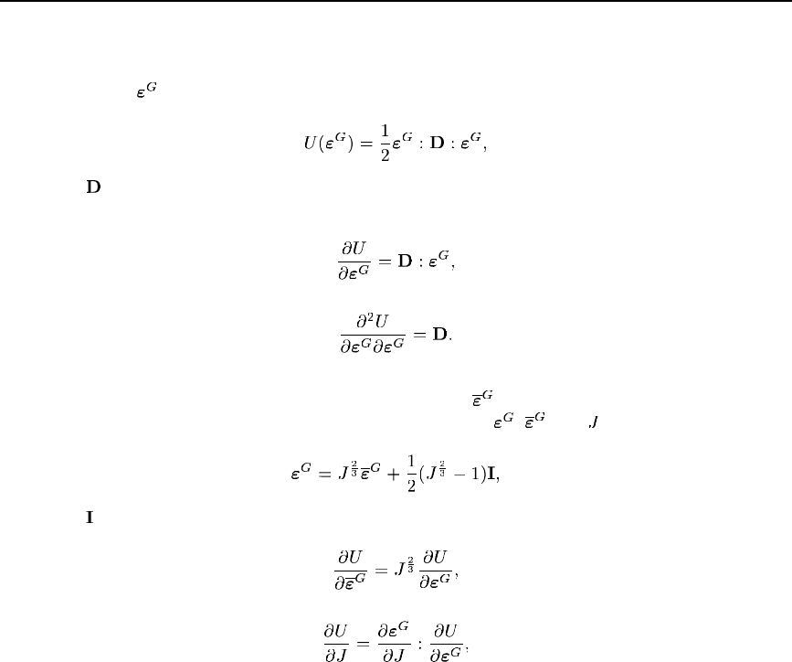
VUANISOHYPER_STRAIN
if (cmname(1:4) .eq. 'MAT1') then
call VUANISOHYPER_STRAIN1(argument_list)
else if (cmname(1:4) .eq. 'MAT2') then
call VUANISOHYPER_STRAIN2(argument_list)
end if
VUANISOHYPER_STRAIN1 and VUANISOHYPER_STRAIN2 are the actual subroutines containing
the anisotropic hyperelastic models for each material MAT1 and MAT2, respectively. Subroutine
VUANISOHYPER_STRAIN merely acts as a directory here. The argument list can be the same as that
used in subroutine VUANISOHYPER_STRAIN. The material nam es must be in uppercase characters
since cmname is passed in as an uppercase character string.
Example: Orthotropic Saint-Venant Kirchhoff model
As a simple example of the coding of subrou tin e VUANISOHYPER_STRAIN, consider the
generalization to anisotropic hyperelasticity of the Saint-Venant Kirchhoff model. The strain energy
function of the S aint-Venant Kirchhoff model can be expressed as a quadratic function of the Green
strain tensor,
,as
where i s the fourth -o rder elastici ty tensor. The derivatives of the strain energy funct ion with re spect
to the G reen strain are given as
However, subroutine VUANISOHYPER_STRAIN m ust return the derivatives of the strain energy
function with respect to the modified Green strain tensor,
, and the volume ratio, J, w hich can be
accomplished easily using the following relationship between
, ,and :
where is the second-order identity tensor. Thus, using the chain rule we find
1.2.11–7
Abaqus ID:
Printed on:

VUANISOHYPER_STRAIN
where
and
In this example an auxiliary function is used to facilitate indexin g into a fourth-order symmetric
tensor. T he subroutine would be coded as follows:
subroutine vuanisohyper_strain (
C Read only -
* nblock,
* jElem, kIntPt, kLayer, kSecPt,
* cmname,
* ndir, nshr, nstatev, nfieldv, nprops,
* props, tempOld, tempNew, fieldOld, fieldNew,
* stateOld, ebar, detu,
C Write only -
* uDev, duDe, duDj,
* d2uDeDe, d2uDjDj, d2uDeDj,
* stateNew )
C
include 'vaba_param.inc'
C
dimension props(nprops),
* tempOld(nblock),
* fieldOld(nblock,nfieldv),
* stateOld(nblock,nstatev),
* tempNew(nblock),
* fieldNew(nblock,nfieldv),
* ebar(nblock,ndir+nshr), detu(nblock),
1.2.11–8
Abaqus ID:
Printed on:
VUANISOHYPER_STRAIN
* uDev(nblock), duDe(nblock,ndir+nshr), duDj(nblock),
* d2uDeDe(nblock,*), d2uDjDj(nblock),
* d2uDeDj(nblock,ndir+nshr),
* stateNew(nblock,nstatev)
C
character*80 cmname
C
parameter( half = 0.5d0, one = 1.d0, two = 2.d0,
* third = 1.d0/3.d0, twothds = 2.d0/3.d0, four = 4.d0,
* dinv = 0.d0 )
C
C Orthotropic Saint-Venant Kirchhoff strain energy function
C (3D)
C
D1111 = props(1)
D1122 = props(2)
D2222 = props(3)
D1133 = props(4)
D2233 = props(5)
D3333 = props(6)
D1212 = props(7)
D1313 = props(8)
D2323 = props(9)
C
dok=1,nblock
C
d2UdE11dE11 = D1111
d2UdE11dE22 = D1122
d2UdE11dE33 = D1133
d2UdE22dE11 = d2UdE11dE22
d2UdE22dE22 = D2222
d2UdE22dE33 = D2233
d2UdE33dE11 = d2UdE11dE33
d2UdE33dE22 = d2UdE22dE33
d2UdE33dE33 = D3333
d2UdE12dE12 = D1212
d2UdE13dE13 = D1313
d2UdE23dE23 = D2323
C
xpow = exp ( log(detu(k)) * twothds )
detuInv = one / detu(k)
C
1.2.11–9
Abaqus ID:
Printed on:
VUANISOHYPER_STRAIN
E11 = xpow * ebar(k,1) + half * ( xpow - one )
E22 = xpow * ebar(k,2) + half * ( xpow - one )
E33 = xpow * ebar(k,3) + half * ( xpow - one )
E12 = xpow * ebar(k,4)
E23 = xpow * ebar(k,5)
E13 = xpow * ebar(k,6)
C
term1 = twothds * detuInv
dE11Dj = term1 * ( E11 + half )
dE22Dj = term1 * ( E22 + half )
dE33Dj = term1 * ( E33 + half )
dE12Dj = term1 * E12
dE23Dj = term1 * E23
dE13Dj = term1 * E13
term2 = - third * detuInv
d2E11DjDj = term2 * dE11Dj
d2E22DjDj = term2 * dE22Dj
d2E33DjDj = term2 * dE33Dj
d2E12DjDj = term2 * dE12Dj
d2E23DjDj = term2 * dE23Dj
d2E13DjDj = term2 * dE13Dj
C
dUdE11 = d2UdE11dE11 * E11
* + d2UdE11dE22 * E22
* + d2UdE11dE33 * E33
dUdE22 = d2UdE22dE11 * E11
* + d2UdE22dE22 * E22
* + d2UdE22dE33 * E33
dUdE33 = d2UdE33dE11 * E11
* + d2UdE33dE22 * E22
* + d2UdE33dE33 * E33
dUdE12 = two * d2UdE12dE12 * E12
dUdE23 = two * d2UdE23dE23 * E23
dUdE13 = two * d2UdE13dE13 * E13
C
U = half * ( E11*dUdE11 + E22*dUdE22 + E33*dUdE33 )
* + E12*dUdE12 + E13*dUdE13 + E23*dUdE23
uDev(k) = U
C
duDe(k,1) = xpow * dUdE11
duDe(k,2) = xpow * dUdE22
duDe(k,3) = xpow * dUdE33
1.2.11–10
Abaqus ID:
Printed on:
VUANISOHYPER_STRAIN
duDe(k,4) = xpow * dUdE12
duDe(k,5) = xpow * dUdE23
duDe(k,6) = xpow * dUdE13
C
xpow2 = xpow * xpow
C Only update nonzero components
d2uDeDe(k,indx(1,1)) = xpow2 * d2UdE11dE11
d2uDeDe(k,indx(1,2)) = xpow2 * d2UdE11dE22
d2uDeDe(k,indx(2,2)) = xpow2 * d2UdE22dE22
d2uDeDe(k,indx(1,3)) = xpow2 * d2UdE11dE33
d2uDeDe(k,indx(2,3)) = xpow2 * d2UdE22dE33
d2uDeDe(k,indx(3,3)) = xpow2 * d2UdE33dE33
d2uDeDe(k,indx(4,4)) = xpow2 * d2UdE12dE12
d2uDeDe(k,indx(5,5)) = xpow2 * d2UdE23dE23
d2uDeDe(k,indx(6,6)) = xpow2 * d2UdE13dE13
C
duDj(k) = dUdE11*dE11Dj + dUdE22*dE22Dj + dUdE33*dE33Dj
* + two * ( dUdE12*dE12Dj + dUdE13*dE13Dj
* + dUdE23*dE23Dj )
d2uDjDj(k)= dUdE11*d2E11DjDj+dUdE22*d2E22DjDj
* +dUdE33*d2E33DjDj
* + two*(dUdE12*d2E12DjDj+dUdE13*d2E13DjDj
* +dUdE23*d2E23DjDj)
* + d2UdE11dE11 * dE11Dj * dE11Dj
* + d2UdE22dE22 * dE22Dj * dE22Dj
* + d2UdE33dE33 * dE33Dj * dE33Dj
* + two * ( d2UdE11dE22 * dE11Dj * dE22Dj
* + d2UdE11dE33 * dE11Dj * dE33Dj
* + d2UdE22dE33 * dE22Dj * dE33Dj )
* + four * ( d2UdE12dE12 * dE12Dj * dE12Dj
* d2UdE13dE13 * dE13Dj * dE13Dj
* d2UdE23dE23 * dE23Dj * dE23Dj )
C
d2uDeDj(k,1) = xpow * ( term1 * dUdE11
* + d2UdE11dE11 * dE11Dj
* + d2UdE11dE22 * dE22Dj
* + d2UdE11dE33 * dE33Dj )
d2uDeDj(k,2) = xpow * ( term1 * dUdE22
* + d2UdE22dE11 * dE11Dj
* + d2UdE22dE22 * dE22Dj
* + d2UdE22dE33 * dE33Dj )
d2uDeDj(k,3) = xpow * ( term1 * dUdE33
1.2.11–11
Abaqus ID:
Printed on:
VUANISOHYPER_STRAIN
* + d2UdE33dE11 * dE11Dj
* + d2UdE33dE22 * dE22Dj
* + d2UdE33dE33 * dE33Dj )
d2uDeDj(k,4) = xpow * ( term1 * dUdE12
* + two * d2UdE12dE12 * dE12Dj )
d2uDeDj(k,5) = xpow * ( term1 * dUdE23
* + two * d2UdE23dE23 * dE23Dj )
d2uDeDj(k,6) = xpow * ( term1 * dUdE13
* + two * d2UdE13dE13 * dE13Dj )
end do
C
return
end
C
integer function indx( i, j )
C
include 'vaba_param.inc'
C
C Function to map index from Square to Triangular storage
C of symmetric matrix
C
ii = min(i,j)
jj = max(i,j)
C
indx = ii + jj*(jj-1)/2
C
return
end
1.2.11–12
Abaqus ID:
Printed on:

VUCHARLENGTH
1.2.12 VUCHARLENGTH: User subroutine to define characteristic element length at a
material point.
Product:
Abaqus/Explicit
References
• *
CHARACTERISTIC LENGTH
•
“VUCHARLENGTH,” Section 4.1.32 of the A baqus Verification Guide
Overview
User subro utine VUCHARLENGTH:
•
is called at all material points of elements for which the mat e rial definition includes a user-defined
characteristic element length and the constitutive model requires a characteristic length;
•
allows the definition of characteristic element length at a material point as a function o f element
topology, nodal and material point coordinates, and material orientation;
•
can use field variables that are passed in; and
•
can use solution-dependent state v ariab les that are passed in.
Defining characteristic element length
The characteristic element length defined in u ser subroutine VUCHARLENGTH is used by Abaqus
in regularization schemes needed to m itigate m esh depen dency in constitutive mod els that include
strain-softening, such as damag e models (“Damage evolution and element removal for ductile metals,”
Section 24.2.3 of the Abaqus Analysis User’s Guide), and concrete (“Concrete smeared cracking,”
Section 23.6.1 of the Abaqus Analysis User ’s Guide). It could be used wi th built -i n Abaqus material
models as well as user subroutine–based material models.
The characteristic eleme nt length coming in user subroutine VUCHARLENGTH has a default value
based on the geometric mean. This default value is a typical leng th of a line across an element for a
first-order elem ent and is half of the same typical length for a second-order element. For trusses the
default value is a characteristic length along the element axis. For m embranes and shells the default
value is a characteristic length in the reference surface. For axisymmetric elements the default value is
a characteri s tic length in th e r–z plane only.
Inside us er subroutine VUCHARLENGTH you can redefine the value of the c har acter isti c element
length based on t he element topology a n d geometry. The characteristic element length definedinuser
subroutine VUCHARLENGTH at a particular material point is passed t o other user subroutines that are
called at the same material point, such as user subroutines VFABRIC, VUMAT, VUSDFLD,andVUEOS.
The characteristic element length calculated in user subroutine VUCHARLENGTH at a particular material
point is also used in built-i n Abaqus material models that require characteristic length and are called at
the sam e material point.
1.2.12–1
Abaqus ID:
Printed on:

VUCHARLENGTH
Array of element type and geometric properties
jElType contains information abou t the element type and th e geometry. jElType(1) provides
information about the shape of the element.
jElType(1) Shape
1 line
2triangle
3 quadrilateral
4 tetrahedron
5wedge
6 hexahedron
jElType(2) provides inform ation about the element’s dimensionality.
jElType(2) Space
1 2D and plane strain
23D
3axisymmetric
4planestress
jElType(3) provides information about the section of the elemen t.
jElType(3) Section
1solid
2shell
3truss
4 m embrane
Elements
User subroutine VUCHARLENGTH can be used with mem brane elements; shell elements; truss elements;
and plane stress, plane strain, axisymmetric, and three-dime nsional solid elements.
Special consideration for 8-node continuum shell elements
For 8-node hexahedron continuum shell elements (SC8R and SC8RT), t he order of nodes in the array of
nodal coordinates (coordNode) passed to user subroutine VUCHARLENGTH dep ends on the stacking
1.2.12–2
Abaqus ID:
Printed on:

VUCHARLENGTH
direction. For a single element nodes 1–4 correspond to the bottom face and nodes 5–6 correspond to
the top face.
User subroutine interface
subroutine vucharlength(
c Read only variables-
1 nblock, nfieldv, nprops, ncomp, ndim, nnode, nstatev,
2 kSecPt, kLayer, kIntPt, jElType, jElem,
3 totalTime, stepTime, dt,
4 cmname, coordMp, coordNode, direct, T, props,
5 field, stateOld,
c Write only variables-
6 charLength )
c
include 'vaba_param.inc'
c
dimension jElType(3), jElem(nblock), coordMp(nblock,ndim),
1 coordNode(nblock,nnode,ndim),
2 direct(nblock,3,3), T(nblock,3,3), props(nprops),
3 stateOld(nblock,nstatev), charLength(nblock,ncomp),
4 field(nblock, nfieldv)
c
character*80 cmname
c
do100k=1,nblock
user coding to define charLength(nblock,ncomp)
100 continue
c
return
end
Variable to be defined
charLength(nblock,ncomp)
Characteristic element length.
Variables passed in for information
nblock
Number of material points to be processed in this call to user subroutine VUCHARLENGTH.
1.2.12–3
Abaqus ID:
Printed on:
VUCHARLENGTH
nfieldv
Number of user-defined external field variables.
nprops
User-specified number of user-defined material properties.
ncomp
User-specified number of components of character isti c el e men t length. If ncomp is greater than 1,
only the first component of characteristic element length would be used in the bui lt- in Abaqus material
models. However, all the com ponents could be used in the above-mentioned user subroutines.
ndim
Number of coordinate directions: 2 for two-dimensional models and 3 for three-dimensional models.
nnode
Number of nodes of the element.
nstatev
Number of user-defined s tate variables that are associated with this material type (define this as
described in “Allocating space” in “User subroutines: overview,” Section 1 8.1.1 of the Abaqus
Analysis User’s Guide).
kSecPt
Section point number within the c urren t layer.
kLayer
Layer number (for composite shells).
kIntPt
Integration point number.
jElType(3)
Array containing information about the element type and geometry.
jElem(nblock)
Array of elem e nt numb ers.
totalTime
Value of total time. The time at the begin nin g of the step is given by totalTime-stepTime.
stepTime
Value of t ime sin ce the step began.
dt
Time increment size.
1.2.12–4
Abaqus ID:
Printed on:

VUCHARLENGTH
cmname
User-specified material name, left justified. It is passed in as an uppercase character string.
coordMp(nblock,ndim)
Material point coordinates. It is the midp lane mater ial point for shell elements.
coordNode(nblock,nnode,ndim)
Nodal coordinates.
direct(nblock,3,3)
An array containing the direction cosines of the material direction s in terms of the global b a sis
directions. For material point k direct(k,1,1), direct(k,2,1),anddirect(k,3,1) give
the (1, 2, 3) components of the first material dir ection; direct(k,1,2), direct(k,2,2),and
direct(k,3,2) give the second material direction and so on. For shell and mem brane elements
the first two directions are in the plane o f the element and the third direction is the normal.
T(nblock,3,3)
An array containing t he direction cosines of the material orientation components relative to the
element basis directions. For material point k this is the orientation that defines the m ater ial directions
(direct) in terms of the element basis directions. For continuum elements T and direct are
identical. For shell and m embrane elements T(k,1,1)
, T(k,1,2) , T(k,2,1)
, T(k,2,2) , T(k,3,3) , and all other components are zero, where is the
counterclockwise rotation around the normal vector that defines the orien tation. If no orientation is
used, T is an identity matrix.
props(nprops)
User-supplied m aterial properties.
field(nblock,nfieldv)
Values of the user- defined field variables at each material point at the beginning o f the increment. User
subroutine VUCHARLENGTH is called before user subroutine VUSDFLD. Thus, any changes to the field
variables made i n user subroutine VUSDFLD are not available in user subroutine VUCHARLENGTH.
stateOld (nblock, nstatev)
State variables at each material point at the beginning of the increment.
1.2.12–5
Abaqus ID:
Printed on:

VUCREEPNETWORK
1.2.13 VUCREEPNETWORK: User subroutine to define time-dependent behavior (creep)
for models defined within the parallel rheological framework.
Product:
Abaqus/Explicit
References
•
“Parallel rheological framework,” Section 22.8.2 of the Abaqus Analysis User’s Guide
•
“Nonlinear large-strain viscoelastici ty with hyperelast icit y,” Section 2.2.8 of the Abaqus
Ver ification Guide
• *
VISCOELASTIC
Overview
User subrou tin e VUCREEPNETWORK:
•
is intended to provide creep law s for nonlinear viscoelastic network s for mod els defined using the
parallel rheological framework;
•
can use and update solution-depen dent state variables; and
•
can be used in conjunctionwithusersubroutineVUSDFLD to rede fine an y field variables before
they are passed in.
Model description
Theusersubroutineallowsacreeplawof the following general form to be defined:
where
and
is th e identity tensor,
is the right Cauchy-Green creep strain tensor,
is the equivalen t creep str ain rate,
is the equivalent creep strain,
is the first invariant of ,
is the second invariant of ,
is the determinant of the deformation gradient, ,
is the Kirchhoff pressure,
1.2.13–1
Abaqus ID:
Printed on:

VUCREEPNETWORK
is the equivalent deviatoric Kirchhoff stress,
t is the time,
is the temperature, and
FV are field variables.
The left Cauchy-Green strain tensor,
,isdefined as
where is the deformation gradient with volume ch a nge eliminated, which is computed u sing
The user subroutine must define the increment of creep equivalent strain, , as a function of the time
increment,
, and the variables used in the definition of , as well as the derivatives of the equivalent
creep strain increment with respect to those variables. If any solution-dependent state variables are
included in the definition of
, they m ust also be integrated forward in time in this user subroutine.
User subroutine interface
subroutine vucreepnetwork (
C Read only -
* nblock, networkid, nstatev, nfieldv,
* nprops, nDg, stepTime, totalTime, dt,
* jElem, kIntPt, kLayer, kSecPt, cmname,
* props, coordMp, tempOld, fieldOld,
* stateOld, tempNew, fieldNew,
* nIarray, i_array, nRarray, r_array,
* q, p, eqcs, TrCc,
C Write only -
* dg, stateNew )
C
include 'vaba_param.inc'
C
C indices for equivalent creep strain and its derivatives
parameter( i_deqcs = 1,
* i_DdeqcsDq = 2,
* i_DdeqcsDeqcs = 3,
* i_DdeqcsDi1c = 4 )
C
C indices for strain invariants
parameter( i_I1 = 1,
* i_I2 = 2,
1.2.13–2
Abaqus ID:
Printed on:

VUCREEPNETWORK
* i_J = 3 )
C
dimension props(nprops),
* tempOld(nblock),
* fieldOld(nblock,nfieldv),
* stateOld(nblock,nstatev),
* tempNew(nblock),
* fieldNew(nblock,nfieldv),
* coordMp(nblock,*),
* jElem(nblock),
* i_array(nblock,nIarray),
* r_array(nblock,nRarray),
* q(nblock),
* p(nblock),
* eqcs(nblock),
* TrCc(nblock),
* stateNew(nblock,nstatev),
* dg(nblock,nDg)
character*80 cmname
C
do 100 km = 1,nblock
user coding
100 continue
return
end
Variables to be defined
dg(nblock,i_deqcs)
Equivalent creep strain increment,
.
dg(nblock,i_DdeqcsDq)
The derivative:
.
dg(nblock,i_DdeqcsDeqcs)
The derivative:
.
dg(nblock,i_DdeqcsDi1c)
The first invariant,
, o f the right Cauchy-Green creep strain tensor, .
1.2.13–3
Abaqus ID:
Printed on:

VUCREEPNETWORK
Variable that can be updated
stateNew(nblock,nstatev)
Array containing the user -defin
ed solution-dependent state variables at this point.
Variables passed in for information
nblock
Number o f material poin ts to b e processed in this call to user subrou tin e VUCREEPNETWORK.
networkid
Network identification number, which identifies the network for which creep is defined.
nstatev
Number of user-defined state variables that are associated with this material type (see “Allocating
space” in “U ser subroutines: overview,” Section 18.1.1 o f the Abaqus Analysis User’s Guide).
nfieldv
Number of user-defined external field variables.
nprops
User-specified number of user-defined material properties.
nDg
Size of array dg.
stepTime
Value of t ime sin ce the step began.
totalTime
Value of total time. The time at the begin nin g of the step is given by totalTime-stepTime.
dt
Time increment size.
jElem(nblock)
Array of elem e nt numb ers.
kIntPt
Integration point number.
kLayer
Layer number (for composite shells).
kSecPt
Section point number within the c urren t layer.
1.2.13–4
Abaqus ID:
Printed on:

VUCREEPNETWORK
cmname
Material name, left justified. It is passed in as an uppercase character string. Some internal material
models are given names start ing with the “ABQ_” character string. To avoid conflict, “ABQ_” should
not be used as the leading string for cmname.
props(nprops)
User-supplied m aterial properties.
coordMp(nblock,*)
Material point coordinates. It is the midplane material point for shell elements and the centroid for
beam elements.
tempOld(nblock)
Temperatures at the material points at th e beginning of the increment.
fieldOld(nblock,nfieldv)
Values of the user-defined field variables at the material points at the beginning of the increm ent.
stateOld(nblock,nstatev)
State variables at the material points at the beginning of the increment.
tempNew(nblock)
Temperatures at the material points at the end o f the increm ent.
fieldNew(nblock)
Values of the user-defined field variables at the material points at the end of the increment.
nIarray
Size of array i_array.
i_array(nblock,nIarray)
Array containing integer arguments. Currently it is not used.
nRarray
Size of array r_array.
r_array(nblock,i_I1)
The first invariant,
, of the left Cauchy-Green strain tensor, .
r_array(nblock,i_I2)
The second invariant,
, of the left Cauchy-Green strain tensor, .
r_array(nblock,i_J)
The determinant o f the deformation gradient,
.
1.2.13–5
Abaqus ID:
Printed on:

VUCREEPNETWORK
q(nblock)
Array containing equivalent deviatoric Kirchhoff stresses.
p(nblock)
Array containing Kirchhoff pressures.
eqcs(nblock)
Array contai ning equivalen t creep st rain s.
TrCc(nblock)
Array containing the first invariants,
, of t he right Cau chy-Green creep strain tensor, .
Example: Power-law strain hardening model
As an example of the coding of user subroutine VUCREEPNETWORK, consider the power-law strain
hardening model. In this case t he equiv alent creep strain rate is expressed as
where
is the equivalent creep strain,
is the equivalent dev iatoric Kirchhoff stress, and
A, m,andn are material parameters.
The user subroutine would be coded as fo llo ws:
subroutine vucreepnetwork (
C Read only -
* nblock, networkid, nstatev, nfieldv,
* nprops, nDg, stepTime, totalTime, dt,
* jElem, kIntPt, kLayer, kSecPt, cmname,
* props, coordMp, tempOld, fieldOld,
* stateOld, tempNew, fieldNew,
* nIarray, i_array, nRarray, r_array,
* q, p, eqcs, TrCc,
C Write only -
* dg, stateNew )
C
include 'vaba_param.inc'
C
parameter ( one = 1.d0, half = 0.5d0 )
parameter ( eqcsSmall = 1.d-8 )
parameter ( rMinVal = 1.d-12 )
1.2.13–6
Abaqus ID:
Printed on:
VUCREEPNETWORK
C
parameter( i_deqcs = 1,
* i_DdeqcsDq = 2,
* i_DdeqcsDeqcs = 3,
* i_DdeqcsDi1c = 4 )
C
dimension props(nprops),
* tempOld(nblock),
* fieldOld(nblock,nfieldv),
* stateOld(nblock,nstatev),
* tempNew(nblock),
* fieldNew(nblock,nfieldv),
* coordMp(nblock,*),
* jElem(nblock),
* i_array(nblock,nIarray),
* r_array(nblock,nRarray),
* q(nblock),
* p(nblock),
* eqcs(nblock),
* TrCc(nblock),
* stateNew(nblock,nstatev),
* dg(nblock,nDg)
C
character*80 cmname
C
C Read properties
C
rA = props(1)
rN = props(2)
rM = props(3)
C
C Update equivalent creep strain and its derivatives
C
dok=1,nblock
om1=one/(one+rM)
test = half - sign( half, q(k) - rMinVal )
qInv=(one-test)/(q(k) + test )
eqcs_t = eqcs(k)
if ( eqcs_t .le. eqcsSmall .and. q(k).gt.rMinVal ) then
C Initial guess based on constant creep strain rate during increment
eqcs_t = dt*(exp(log(rA)+rN*log(q(k)))*
* ((one+rM)*dt)**rM)
1.2.13–7
Abaqus ID:
Printed on:
VUCREEPNETWORK
end if
C
test2 = half - sign( half, eqcs_t - rMinVal )
eqcsInv = ( one - test2)/(eqcs_t + test2 )
g = dt*(exp(log(rA)+rN*log(q(k)))*
* ((one+rM)*(test2+eqcs_t))**rM)**om1
dg(k,i_deqcs) = g
dg(k,i_DdeqcsDq) = qInv * rN * om1 * g
dg(k,i_DdeqcsDeqcs) = eqcsInv * rM * om1 * g
end do
C
return
end
1.2.13–8
Abaqus ID:
Printed on:

VUEL
1.2.14 VUEL: User subroutine to define an element.
Product:
Abaqus/Explicit
WARNING : This feature is intended for advanced users only. Its use in all but the
simplest test examples will require considerable coding by the user/developer.
“User-defined elements,” Section 32.17.1 o f the Abaqus Analysis User’s Guide,
should be read before proceeding.
References
•
“User-defined elements,” Section 32.17.1 of the Abaq us Analysis User’s Guide
•
“User-defined element library,” S ection 32 .1 7.2 of the Abaq us Analysis User’s Guide
•
“UEL,” Section 1.1.28
• *
UEL PROPERTY
• *
USER ELEMENT
Overview
User subroutine VUEL:
•
will be called f or each element that is of a general user-defined element type each time elem ent
calculations are required; and
•
(or subro utines called by user subroutine VUEL) must perform all of the calculations for the element,
appropriate to the current activity in the analysis.
User subroutine interface
SUBROUTINE VUEL(nblock,rhs,amass,dtimeStable,svars,nsvars,
1 energy,
2 nnode,ndofel,props,nprops,jprops,njprops,
3 coords,mcrd,u,du,v,a,
4 jtype,jElem,
5 time,period,dtimeCur,dtimePrev,kstep,kinc,
6 lflags,
7 dMassScaleFactor,
8 predef,npredef,
9 jdltyp, adlmag)
C
include 'vaba_param.inc'
C operational code keys
1.2.14–1
Abaqus ID:
Printed on:
VUEL
parameter ( jMassCalc = 1,
* jIntForceAndDtStable = 2,
* jExternForce = 3)
C flag indices
parameter (iProcedure = 1,
* iNlgeom = 2,
* iOpCode = 3,
* nFlags = 3)
C energy array indices
parameter ( iElPd = 1,
* iElCd = 2,
* iElIe = 3,
* iElTs = 4,
* iElDd = 5,
* iElBv = 6,
* iElDe = 7,
* iElHe = 8,
* iElKe = 9,
* iElTh = 10,
* iElDmd = 11,
* iElDc = 12,
* nElEnergy = 12)
C predefined variables indices
parameter ( iPredValueNew = 1,
* iPredValueOld = 2,
* nPred = 2)
C time indices
parameter (iStepTime = 1,
* iTotalTime = 2,
* nTime = 2)
dimension rhs(nblock,ndofel),amass(nblock,ndofel,ndofel),
1 dtimeStable(nblock),
2 svars(nblock,nsvars),energy(nblock,nElEnergy),
3 props(nprops),jprops(njprops),
4 jElem(nblock),time(nTime),lflags(nFlags),
5 coords(nblock,nnode,mcrd),
6 u(nblock,ndofel), du(nblock,ndofel),
1.2.14–2
Abaqus ID:
Printed on:

VUEL
7 v(nblock,ndofel), a(nblock, ndofel),
8 dMassScaleFactor(nblock),
9 predef(nblock,nnode,npredef,nPred),
* adlmag(nblock)
do kblock = 1,nblock
user coding to define rhs, amass, dtimeStable, svars and energy
end do
RETURN
END
Variables to be defined
Some of the following arrays depend on the value of the lflags array.
rhs
An array containing the contributions of each element to the right-hand-side vector of the overall system
of equations. Depending on the settings of the lflags array, it contains either the internal force from
the element or the external load calculated from the specified distributed loads.
amass
An array containing the contribution of each element to the mass matrix of the overall system of
equations.
All nonzero entries in amass should be defined. Moreover, the mass matrix must be sy mm etric.
There are several other requireme nts that apply depending on the active degrees of freedom specified.
These requirements are explained in detail below.
dtimeStable
A scalar value defining, for each element, the upper limit of the time increment for stability
considerations. This would be the maximum time increment to be used in the subsequent increment
for this element to be stable (to satisfy the Courant condition). This value depends strongly on the
element formulation, and it is important th at is computed appropriately.
svars
An array containing the values of the solution-dependent state variables associated with each element.
The number of such variables is nsvars (see below). You define the meaning of these variables.
ThisarrayispassedintoVUEL containing the values of these variables at the start o f the current
increment. In most cases they should be updated to be the values at the end of the increment. In rare
cases such an update is not required.
energy
The array energy contains the values of the energy quantities associated with each element. The
values in this array when VUEL is called are the element energy quantities at the start of the current
1.2.14–3
Abaqus ID:
Printed on:

VUEL
increment. They should be updated to the correct values at the end of the current increment; otherwise,
plots of the energy balance for the entire model will not be accurate. Depending on the e lem ent
formulation, many o f these energies could be zero at all times. The entries in the array are as fol lows:
energy(nblock,iElPd ) Plastic dissipation.
energy(nblock,iElCd) Creep d issipation.
energy(nblock,iElIe) Internal energy.
energy(nblock,iElTs) Transverse shear energy.
energy(nblock,iElDd) Material damping
dissipation.
energy(nblock,iElBv) Bulk viscosity
dissipation.
energy(nblock,iElDe) Drill energy.
energy(nblock,iElHe) Hourglass energy.
energy(nblock,iElKe) Kinetic energy.
energy(nblock,iElTh) Heat energy.
energy(nblock,iElDmd) Damage dissipation.
energy(nblock,iElDc ) Distortion control
energy.
Variables passed in for information
Arrays:
props
A floating point array containing the nprops real property values defined for use with each element
processed. nprops is the user-specified number of real property values. See “Defining the element
properties” in “User-defined elements,” Section 32.17.1 of the Abaqus Analysis User’s Guide.
jprops
An integer array containing the njprops integer property values defined for use with each element
processed. njprops is the user-specified nu mb er of integer property values. See “De fining the
element properties” in “User-defined elements,” Section 32.17 .1 of the Abaqus Analysis User’s Guide.
coords
An array containing the original coordinates of the nodes of the element. coords(kblock,k1,k2)
is the k2th coordinate of the k1th nod e of t he kblock element.
1.2.14–4
Abaqus ID:
Printed on:
VUEL
u, du, v, a
Arrays containing the basic solution variables (displacements, rotations, temperatures, pressures,
depending on the degree of freedom) at th e nodes of the element. Values are prov ided as follows,
illustrated below for the k1th degree of freedom of the kblock element:
u(kblock,k1) Total value o f the variables (such as
displacements or rotations) at the end of
the current increment.
du(kblock,k1) Incremental values of the variables in the
current increment.
v(kblock,k1) Time rate of change of the variables
(velocities, rat es of rotation) at the
midpoint of the increment.
a(kblock,k1) Accelerations of the variables at the end
of the current increment.
jElem
jElem(kblock) co ntains the element number for t he kblock element.
adlmag
adlmag(kblock) is the total load magnitude of the load type jdltyp (int eger identifying the load
number for distributed load ty pe Un) distributed load at the end of the current increment for distributed
loads of type Un.
predef
An array containing the values of predefined field variables, such as temperature in an uncoupled
stress/displacement analysis, at the nodes of the element (“Predefined fields,” Section 34.6.1 of the
Abaqus Analysis User’s Guide).
The seco nd index, k2, indicates the local node number on the kblock element. The third index,
k3, indicates the variable: the temperature is stored if the index is 1, and the predefined field variables
are stored if the indices are g reater than or equal to 2. The fourth index of the array, k4, is either 1 or
2, with 1 indicating the value of the field variable at the end of the increment and 2 indicating the value
of the field variable at the beginning of the increment.
predef(kblock,k2,1,k4) Temperature.
predef(kblock,k2,2,k4) First predefined field variable.
predef(kblock,k2,3,k4) Second predefined field variable.
Etc. Any other predefined field
variable.
1.2.14–5
Abaqus ID:
Printed on:
VUEL
predef(kblock,k2,k3,k4) Va l u e of t he (k3–1)th predefined
field variable at the k2th node of
the element at the beginning or
the end of the increment.
predef(kblock,k2,k3,1) Values of the variables at the end
of the current increment.
predef(kblock,k2,k3,2) Values of the variables at
the beginning of the curren t
increment.
lflags
An array containing the flags that define the current solution procedu re and requirements for element
calculations.
lflags(iProcedure) Defines the procedure type. See
“Results file output format,”
Section 5.1.2 of the Abaqus Analysis
User’s G uide, for the key used for each
procedure.
lflags(iNlgeom)=0 Small-displacement analysis.
lflags(iNlgeom)=1 Large-displacement analysis (nonlinear
geometric effects included in the step;
see “General and linear perturbation
procedures,” Section 6.1.3 of the
Abaqus Analysis User’s Guide).
lflags(iOpCode)=jMassCalc Define the mass matrix amass in the
beginning of the analysis.
lflags(iOpCode)=jIntForceAnd-
DtStable
Define the element internal force.
Define the stab le time increment as
well.
lflags(iOpCode)=jExternForce Define the distributed load effect on
the external f orce associated with the
element.
dMassScaleFactor
An array containing the mass scale factors for each element.
time(iStepTime)
Current value of step time.
1.2.14–6
Abaqus ID:
Printed on:
VUEL
time(iTotalTime)
Current value of total time.
Scalar parameters:
nblock
Number of user elements to be processed in this call to VUEL.
dtimeCur
Current time increment.
dtimePrev
Previous time increment.
period
Time period o f the current step.
ndofel
Number of degrees of freedom in the elements processed.
nsvars
User-defined n um ber of solution-dependent s tate variables associated with the element (“Defining
the number of solution-d epend ent variables th at must be stored withi n the element” in “User-defined
elements,” Section 32.17.1 of the Abaq us Analysis User’s Guide).
nprops
User-defined number of real property values associated with the elements processed (“Defining the
element properties” in “User-defined elements,” Section 32.17.1 of the Abaqus Analysis User’s Guide).
njprops
User-defined number of integer property values associated with the elements processed (“Defining the
element properties” in “User-defined elements,” Section 32.17.1 of the Abaqus Analysis User’s Guide).
mcrd
mcrd is defined as the max im um of the user-defined maximum number of coordinates needed at any
node point (“Defining the maximum number of coordin ates needed at any nodal point” in “User-defined
elements,” Section 32.17.1 of the Abaqus Analysis User’s Guide) and the value of the largest active
degree of freedom of the user element that is less than or equal to 3. F or example, if you specify that
the maxim um number of coordinates is 1 and the active degrees of freedom of the user element are 2,
3, and 6 mcrd will be 3. If you specify that the maximum number of coordinates is 2 and the active
degree of freedom of the user elem ent is 11, mcrd will be 2.
nnode
User-defined num ber of nodes on the elements (“Defining the number of nodes a ssociated with the
element” in “User-defined elements,” S ection 32.17.1 of the Abaqus Analysis User’s Gu ide).
1.2.14–7
Abaqus ID:
Printed on:

VUEL
jtype
Integer d e fi ning the element type. T his is the user-defined integ er value n in element type
VUn (“A ssigning an element type key to a user-defined element” in “User-defined elements,”
Section 32.17.1 of th e Ab aqus Analysis User’s Guide).
kstep
Current step number.
kinc
Current i ncrem ent nu mb er.
npredef
Number of predefined field variables, including temperature. For user elements Abaqus/Explicit uses
one value for each field variable per node.
VUEL conventions
The solution variables (displacement, velocity, etc.) are arranged on a node/degree of freedom basis. The
degrees of freedom of the first node are first, followed by the degrees of freedom of the second node, etc.
The degrees of freedom that will be updated automatically in Abaqus/Explicit are: 1–3 (displacements),
4–6 (rotations), 8 (pressu re), and 11 (temperature). Depending on the procedure type (see below), only
some of the degrees of freedom listed above will be updated. O ther degrees of freedom will not be
updated by the time integration procedure in Abaqus/Explicit and, hence, should not be used.
The m ass matrix defined in user subroutine VUEL must be symmetric. In addition, the following
requirements apply:
•
The mass matrix entries associated with the translational degrees of freedom for a particular node
must be diagonal. Moreover, these diagonal entries must be equal to each other.
•
There must be no coupling (off-diagonal) entries specified between degrees of freedom of different
kinds. F or example, you cannot specify nonzero mass matrix entries to couple the translational
degrees of freedom to the rotational degrees of freedom.
•
There must be no coupling (off-diagonal) entries specified between degrees of freedom belonging
to different nodes.
You m ust b e usin g ap pro priate lumping techniques to provide a mass matrix that follows these
requirements. For the rotatio nal degrees of freedom at a particular node in three-dimensional analyses,
you can specify a fully populated symmetric 3 × 3 inertia tensor.
Usage with general nonlinear procedures
The following illustrates the use in explicit dynam ic procedures:
Direct-integration explicit dynamic analysis (lflags(iProcedure)=17)
•
Automatic updates for degrees of freedom 1–6, 8, and 11.
1.2.14–8
Abaqus ID:
Printed on:

VUEL
•
The governing equations are as described in “Explicit dynamic analysis,” Section 6.3.3 of the
Abaqus Analysis User’s Guide.
•
Coding for the operational c od e lflags(iOpCode)=jExternForceis optional.
Transient fully coupled thermal-stress analysis (lflags(iProcedure)=74)
•
Automatic updates for degrees of freedom 1–6 and 11.
•
The governing equations are as described in “Fully coupled thermal-stress analysis in
Abaqus/Explicit” in “Fully cou pled thermal- st ress analysis,” Section 6.5.3 of the A baqus Analysis
User’s Guide.
•
Coding for the operational code lflags(iOpCode)=jExternForce is option a l.
Example: Structural user element
A structural user element has been created to demonstrate the usage of subroutine VUEL. These user-
defined elem ents are applied in a nu mb er of analyses. The following excerpt is fro m the verification
problem that invok es the structural user element in an ex plicit dynamic procedure:
*
USER ELEMENT, NODES=2, TYPE=VU1, PROPERTIES=4, COORDINATES=3,
VARIABLES=12
1, 2, 3
*
ELEMENT, TYPE=VU1
101, 101, 102
*
ELGEN, ELSET=VUTRUSS
101, 5
*
UEL PROPERTY, ELSET=VUTRUSS
0.002, 2.1E11, 0.3, 7200.
The user elem e nt consists of two no des that are assumed to lie parallel to the x-axis. The element behaves
similarly to a linear truss element. The supplied elem ent properties are the cross-sectional area, Young’s
modulus, Poisson’s ratio, and density, respectively.
The n ext excerpt shows the listing of the subroutine. The user subroutine has been coded for use
in an explicit dynamic analysis. The names of the verification input files associated with the sub routine
and these procedures can be found in “VUEL,” Section 4.1.33 of the A baqus Verification Guide.
subroutine vuel(
* nblock,
* rhs,amass,dtimeStable,
* svars,nsvars,
* energy,
* nnode,ndofel,
* props,nprops,
* jprops,njprops,
* coords,ncrd,
* u,du,v,a,
1.2.14–9
Abaqus ID:
Printed on:
VUEL
* jtype,jElem,
* time,period,dtimeCur,dtimePrev,kstep,kinc,lflags,
* dMassScaleFactor,
* predef,npredef,
* ndload,adlmag)
include 'vaba_param.inc'
c operation code
parameter ( jMassCalc = 1,
* jIntForceAndDtStable = 4)
c flags
parameter (iProcedure = 1,
* iNlgeom = 2,
* iOpCode = 3,
* nFlags = 3)
c procedure flags
parameter ( jDynExplicit = 17 )
c time
parameter (iStepTime = 1,
* iTotalTime = 2,
* nTime = 2)
c energies
parameter ( iElPd = 1,
* iElCd = 2,
* iElIe = 3,
* iElTs = 4,
* iElDd = 5,
* iElBv = 6,
* iElDe = 7,
* iElHe = 8,
* iElKe = 9,
* iElTh = 10,
* iElDmd = 11,
* iElDc = 12,
* nElEnergy = 12)
parameter (factorStable = 0.99d0)
1.2.14–10
Abaqus ID:
Printed on:
VUEL
parameter (zero = 0.d0, half = 0.5d0, one = 1.d0, two=2.d0)
C
dimension rhs(nblock,ndofel), amass(nblock,ndofel,ndofel),
* dtimeStable(nblock),
* svars(nblock,nsvars), energy(nblock,nElEnergy),
* props(nprops), jprops(njprops),
* jElem(nblock), time(nTime), l(nFlags),
* coords(nblock,nnode,ncrd), u(nblock,ndofel),
* du(nblock,ndofel), v(nblock,ndofel), a(nblock, ndofel),
* predef(nblock, nnode, npredef, nPred), adlmag(nblock),
* dMassScaleFactor(nblock)
c Notes:
c Define only nonzero entries; the arrays to be defined
c have been zeroed out just before this call
if (jtype .eq. 1001 .and.
* lflags(iProcedure).eq.jDynExplicit) then
area0 = props(1)
eMod = props(2)
anu = props(3)
rho = props(4)
eDampTra = zero
amassFact0 = half*area0*rho
if ( lflags(iOpCode).eq.jMassCalc ) then
do kblock = 1, nblock
c use original distance to compute mass
alenX0 = (coords(kblock,2,1) - coords(kblock,1,1))
alenY0 = (coords(kblock,2,2) - coords(kblock,1,2))
alenZ0 = (coords(kblock,2,3) - coords(kblock,1,3))
alen0 = sqrt(alenX0*alenX0 + alenY0*alenY0 +
* alenZ0*alenZ0)
am0 = amassFact0*alen0
amass(kblock,1,1) = am0
amass(kblock,2,2) = am0
amass(kblock,3,3) = am0
amass(kblock,4,4) = am0
amass(kblock,5,5) = am0
1.2.14–11
Abaqus ID:
Printed on:
VUEL
amass(kblock,6,6) = am0
end do
else if ( lflags(iOpCode) .eq.
* jIntForceAndDtStable) then
do kblock = 1, nblock
alenX0 = (coords(kblock,2,1) - coords(kblock,1,1))
alenY0 = (coords(kblock,2,2) - coords(kblock,1,2))
alenZ0 = (coords(kblock,2,3) - coords(kblock,1,3))
alen0 = sqrt(alenX0*alenX0 + alenY0*alenY0 +
* alenZ0*alenZ0)
vol0 = area0*alen0
amElem0 = two*amassFact0*alen0
alenX = alenX0
* + (u(kblock,4) - u(kblock,1))
alenY = alenY0
* + (u(kblock,5) - u(kblock,2))
alenZ = alenZ0
* + (u(kblock,6) - u(kblock,3))
alen = sqrt(alenX*alenX + alenY*alenY + alenZ*alenZ)
area = vol0/alen
ak = area*eMod/alen
c stable time increment for translations
dtimeStable(kblock) = factorStable*sqrt(amElem0/ak)
c force=E*logarithmic strain *current area
strainLog = log(alen/alen0)
fElasTra = eMod*strainLog*area
forceTra = fElasTra
c assemble internal load in RHS
rhs(kblock,1) = -forceTra
rhs(kblock,4) = forceTra
c internal energy calculation
alenOld = svars(kblock,1)
fElasTraOld = svars(kblock,2)
energy(kblock, iElIe) = energy(kblock, iElIe) +
1.2.14–12
Abaqus ID:
Printed on:
VUEL
* half*(fElasTra+fElasTraOld)*(alen - alenOld)
c update state variables
svars(kblock,1) = alen
svars(kblock,2) = fElasTra
end do
end if
end if
c
return
end
1.2.14–13
Abaqus ID:
Printed on:

VUEOS
1.2.15 VUEOS: User subroutine to define equation of state material model.
Product:
Abaqus/Explicit
References
•
“Equation of state,” Section 25.2.1 of the Abaqus Analysis User’s Guide
• *
EOS
•
“Equation of state material,” Section 2.2.20 of the Abaqus Verification Guide
Overview
User su bro utine VUEOS:
•
can be used to define the hydrodynamic material model in which the materi al’s volumetric respo n se
is determined by the user-definedequationofstate;
•
will be called for blocks of material calculation points for which the m aterial de fin ition contains a
user-defined equation of state;
•
can use and update solution-depen dent state variables; and
•
can use any field variables that are passed in.
User subroutine interface
subroutine vueos (
C Read only (unmodifiable) variables –
1 nblock,
2 jElem, kIntPt, kLayer, kSecPt,
3 stepTime, totalTime, dt, cmname,
4 nstatev, nfieldv, nprops,
5 props, tempOld, tempNew, fieldOld, fieldNew,
6 stateOld, charLength, coordMp,
7 densityMean, refDensity, densityNew,
8 dkk, Em,
C Write only (modifiable) variables –
8 press, dPdRho, dPdEm,
9 stateNew )
C
include 'vaba_param.inc'
C
dimension props(nprops),
1 tempOld(nblock),
2 fieldOld(nblock,nfieldv),
1.2.15–1
Abaqus ID:
Printed on:

VUEOS
3 stateOld(nblock,nstatev),
4 tempNew(nblock),
5 fieldNew(nblock,nfieldv),
6 charLength(nblock), coordMp(nblock,*),
7 densityMean(nblock), refDensity(nblock),
8 densityNew(nblock),
9 dkk(nblock), Em(nblock),
1 press(nblock),dPdRho(nblock),dPdEm(nblock),
2 stateNew(nblock)
C
character*80 cmname
C
do 100 km = 1,nblock
user coding to define/update press, dPdRho, dPdEm
100 continue
return
end
Variables to be defined
press(nblock)
The material point pressure stress, p.
dPdRho(nblock)
The derivative of the pressure with respect to the density,
. This quantity is needed for the
evaluation of the effective moduli of the material, which enters the stable time increment calculation.
dPdEm(nblock)
The derivative of the pressure wi th r e sp ect to the internal energy,
. This quantity is needed
for the iterative Newton loop used outside of the user subroutine to solve for pressu re.
Variable that can be updated
stateNew(nblock,nstatev)
State variables at each material point at the end of the increment. You define the size of this array by
allocating s pace for it (see “User subroutines: overview,” S ection 18.1.1 of the Abaqus Analysis User’s
Guide, for more information).
1.2.15–2
Abaqus ID:
Printed on:

VUEOS
Variables passed in for information
nblock
Number of material points to be processed in this call to VUEOS.
jElem(nblock)
Array of elem e nt numb ers.
kIntPt
Integration point number.
kLayer
Layer number.
kSecPt
Section point number within the c urren t layer.
stepTime
Value of t ime sin ce the step began.
totalTime
Value o f total time. The time at the beginnin g of the step is given by totalTime - stepTime.
dt
Time increment size.
cmname
User-specified material name, left justified. It is passed in as an uppercase character string. Some
internal material models are given names starting with the “A BQ_” character string. To avoid conflict,
you should not use “ABQ_” as the leading string for cmname.
nstatev
Number of user-defined state variables that are associated with this material type (you define the number
as described in “Allocating space” in “User subroutines: overview,” Section 18.1.1 of the Abaqus
Analysis User’s Guide).
nfieldv
Number of user-defined external field variables.
nprops
User-specified number of user-defined material properties.
props(nprops)
User-supplied m aterial properties.
1.2.15–3
Abaqus ID:
Printed on:

VUEOS
tempOld(nblock)
Temperatures at each m aterial point at the beginning of the increment.
tempNew(nblock)
Temperatures at each material point at the end of the increment.
fieldOld(nblock,nfieldv)
Values of the user-defined field v ariables at each material point at the beginning of the increment.
fieldNew(nblock,nfieldv)
Values of the user-defined field variables at each material point at the end of the increment.
stateOld(nblock,nstatev)
State variables at each material point at the beginning of the increment.
charLength(nblock)
Characteristic element length, which is either the default value based o n the geometric mean or the
user-defined characteristic elem ent length defined in user subroutin e VUCHARLENGTH. The default
value is a typical length of a line across an element for a first-order elem ent; it is half the sam e typical
length for a second-ord er element. For beams, pipes, and trusses, the default value is a characteristic
length al ong the element axis. For m embranes and shells it is a characteristic l engt h in t he referenc e
surface. For axisymmetric elements it is a characteristic length in the r–z plane only. For cohesive
elements it is equal to the constitutive thickness.
coordMp(nblock,*)
Material point coordinates.
densityMean(nblock)
The mean density.
refDensity(nblock)
The reference density.
densityNew(nblock)
The current density for this inc rement.
dkk(nblock)
The volum etric strain increment.
Em(nblock)
The element specific internal energy (per u nit mass)
Example: User subroutine VUEOS to reproduce results obtained with
*
EOS, TYPE=USUP
As a simple exam ple of coding o f user subroutine VUEOS, consider the following form of the Mie-
Grüneisen equation of state with
0.0 and a l inear dependency betw een pressure and internal energy:
1.2.15–4
Abaqus ID:
Printed on:

VUEOS
where . Therefore, the results obtained with user subroutine VUEOS should b e the same as
the results obtained with the linear
type of EOS already available in “Equation of state material,”
Section 2.2.20 of the Abaqus Verification Guide.
The code in user subroutine VUEOS must return the pressure,
, as in the above equation; the
derivative of the pressure with re spect to the density,
; and the derivative of the pressur e with
respect to the energy,
. For the case considered here, these values are
subroutine vueos (
C Read only (unmodifiable) variables –
1 nblock,
2 jElem, kIntPt, kLayer, kSecPt,
3 stepTime, totalTime, dt, cmname,
4 nstatev, nfieldv, nprops,
5 props, tempOld, tempNew, fieldOld, fieldNew,
6 stateOld, charLength, coordMp,
7 densityMean, refDensity, densityNew,
8 dkk, Em,
C Write only (modifiable) variables –
8 press, dPdRho, dPdEm,
9 stateNew )
C
include 'vaba_param.inc'
C
dimension props(nprops),
1 tempOld(nblock),
2 fieldOld(nblock,nfieldv),
3 stateOld(nblock,nstatev),
4 tempNew(nblock),
5 fieldNew(nblock,nfieldv),
6 charLength(nblock), coordMp(nblock,*),
7 densityMean(nblock), refDensity(nblock),
8 densityNew(nblock),
9 dkk(nblock), Em(nblock),
1 press(nblock),dPdRho(nblock),dPdEm(nblock),
1.2.15–5
Abaqus ID:
Printed on:
VUEOS
2 stateNew(nblock)
C
character*80 cmname
C
parameter ( zero = 0.d0, one = 1.d0, half = 0.5d0 )
C
c0 = props(1)
gamma0 = props(2)
c02 = c0*c0
C
do k=1, nblock
rho0 = refDensity(k)
eta = one - rho0/densityNew(k)
f1 = rho0*c02*eta*(one-half*gamma0*eta)
f2 = gamma0*rho0
press(k) = f1 + f2*Em(k)
C dP/dEm
dPdEm(k) = f2
C dP/dRho
dPdRho(k)= c02*(rho0/densityNew(k))**2*(one-gamma0*eta)
end do
C
return
end
1.2.15–6
Abaqus ID:
Printed on:

VUFIELD
1.2.16 VUFIELD: User subroutine to specify predefined field variables.
Product:
Abaqus/Explicit
References
•
“Predefined fields,” Section 34.6.1 of the Abaqus Analysis User ’s Guide
• *
FIELD
Overview
User subroutine VUFIELD:
•
allows you to prescribe predefined field variables at the nodes of a model—the predefined field
variables at a node can b e updated individually, or a number of field variables at the nodes can be
updated simultaneously ;
•
can be called for blocks of nodes for w hich the field variable values are defined in the subrou tine;
•
ignores any field variable values specified directly;
•
can be used to m odify field variable v alues read from a results file; and
•
can be used in conjunction with user subroutine VUSDFLD such that the field variables that are
passed in from VUFIELD and interpo lated to the material points can be m od ifi ed (such changes are
local to material point values, and nodal field variable values remain unaffected).
Updating field variables
Two different methods are provided for updating field variables.
Individual variable updates
By default, only on e field variable is updated at a time for given nodes or a given node set in user
subroutine VUFIELD. The user subroutine is called whenever a current valu e of a field v ariable is needed
for the nodes that are listed in the field variable definition. This method is ideal for cases in w hich the
field variables are independent of each other.
Simultaneous variable updates
User subroutine VUFIELD can also be used to update m ultiple field variables simultaneously for given
nodes o r a given node set. This method is well-suited for cases in which there are dependencies b etween
some of the field variables. In this case you must specify the number of field variables to be updated
simultaneously, and the user subroutine will be called each time the field variable values are needed.
1.2.16–1
Abaqus ID:
Printed on:

VUFIELD
User subroutine interface
SUBROUTINE VUFIELD(FIELD, NBLOCK, NFIELD, KFIELD, NCOMP,
1 KSTEP, JFLAGS, JNODEID, TIME,
2 COORDS, U, V, A)
C
INCLUDE 'VABA_PARAM.INC'
C indices for the time array TIME
PARAMETER( i_ufld_Current = 1,
* i_ufld_Increment = 2,
* i_ufld_Period = 3,
* i_ufld_Total = 4 )
C indices for the coordinate array COORDS
PARAMETER( i_ufld_CoordX = 1,
* i_ufld_CoordY = 2,
* i_ufld_CoordZ=3)
C indices for the displacement array U
PARAMETER( i_ufld_SpaDisplX = 1,
* i_ufld_SpaDisplY = 2,
* i_ufld_SpaDisplZ = 3,
* i_ufld_RotDisplX = 4,
* i_ufld_RotDisplY = 5,
* i_ufld_RotDisplZ = 6,
* i_ufld_AcoPress = 7,
* i_ufld_Temp = 8 )
C indices for the velocity array V
PARAMETER( i_ufld_SpaVelX = 1,
* i_ufld_SpaVelY = 2,
* i_ufld_SpaVelZ = 3,
* i_ufld_RotVelX = 4,
* i_ufld_RotVelY = 5,
* i_ufld_RotVelZ = 6,
* i_ufld_DAcoPress = 7,
* i_ufld_DTemp = 8 )
C indices for the acceleration array A
PARAMETER( i_ufld_SpaAccelX = 1,
1.2.16–2
Abaqus ID:
Printed on:

VUFIELD
* i_ufld_SpaAccelY = 2,
* i_ufld_SpaAccelZ = 3,
* i_ufld_RotAccelX = 4,
* i_ufld_RotAccelY = 5,
* i_ufld_RotAccelZ = 6,
* i_ufld_DDAcoPress = 7,
* i_ufld_DDTemp = 8 )
C indices for JFLAGS
PARAMETER( i_ufld_kInc = 1,
* i_ufld_kPass = 2 )
C
DIMENSION FIELD(NBLOCK,NCOMP,NFIELD)
DIMENSION JFLAGS(2), JNODEID(NBLOCK), TIME(4),
* COORDS(3,NBLOCK)
DIMENSION U(8,NBLOCK), V(8,NBLOCK), A(8,NBLOCK)
C
user coding to define FIELD
RETURN
END
Variable to be defined
FIELD(NBLOCK,NCOMP,NFIELD)
Array of field variable values at a collective num ber of nodes NBLOCK (see NBLOCK below). When
updating one field variable at a time, only the value of the specified fi eld v ariable KFIELD mu st
be returned. In this case NFIELD is passed i nto user subroutine VUFIELD with a value of 1, and
FIELD is thus dimensioned as FIELD(NBLOCK,NCOMP,1). When updating all field variables
simultaneously, the values of the specified number of field variables must be returned. In this case
FIELD is dimensioned as FIELD(NBLOCK,NCOMP,NFIELD),whereNFIELD is the n um ber of
field variables specified and KFIELD,whichissetto−1, has no meaning.
If fields are applied to nodes that are not part of pipe, beam, or shell elem ents, only one value
of each field variable is required (NCOMP=1), an d the user subroutine is invoked in a single pass. For
nodes that are part o f pipe, beam, or shell elements, VUFIELD is invoked in two passes per increment
for these elements, and the num ber o f v alues to be returned depends on the mode of tem perature and
field variable input selected for the beam or shell section. The following cases are possible:
1. Field variables are given as values at the points on the shell or beam section. For a beam section
the number of values required is determined by the particular sectio n type specified, as described
in “Beam cross-section library,” Section 29.3.9 of the Abaqus Analysis Us er’s Guide. For a shell
section temperatures and field variables are given as values at n equally spaced points through
1.2.16–3
Abaqus ID:
Printed on:

VUFIELD
each layer of a shell s ection. In the fi rst pass NCOMP is passed in wi th the value o f 1 to define
the field variable values at the first poin t. The secon d pass is used to define field variables at the
remaining p oints.
2. Field variables for the shell or beam section are given as values at the origin of the cross-section
together w ith gradients al ong the cr oss-secti on. The number o f gradient values required is 2 for
three-dimensional beams, 1 f or two-dimensional beam s, and 1 for shells. In the first pass NCOMP
is passed in with th e value of 1 to defi ne the field variable valu e s at the origin of the cross-section.
The gradients are definedinthesecondpass.
Because field variables can also be defined directly, it is imp ortant to understand the hierarchy
used in situations with conflicting i nform a tion (see “Predefined fields,” Section 34.6.1 of the Abaq us
Analysis User’s Guide).
When the array FIELD is passed into user subroutine VUFIELD,itwillcontaineitherthefield
variable values from the p revious increment or those values obtained from t he results file if this met hod
was used. You can then modify these values within this subroutine.
Variables passed in for information
NBLOCK
User-specified number of nodes to be processed as a block in this call to VUFIELD. The value is equal
to the total n um ber of nodes given in a node set when blocking is disabled. When blocking is enabled,
NBLOCK is equal to a predefined num ber set in A baqu s/Explicit. You can also modify NBLOCK by
specifying a b locking size in the Abaqus/Explicit analysis.
NFIELD
User-specified number of fi eld variables to be updated. The default value is 1.
KFIELD
User-specified field variable number. This variable is meaningful only when updating individual field
variables at a time; otherwise, the value i s set to −1.
NCOMP
Maximum number of section values to be d efi ned for any node in the model in t he current pass. The
first pass to user subroutine VUFIELD has NCOMP passed in with the value of 1.
KSTEP
Current step number.
JFLAGS(i_ufld_kInc)
Increment number for step KSTEP.
JFLAGS(i_ufld_kPass)
This flag is equal to 1 for the first pass to user subroutine VUFIELD and is equal to 2 for the second
pass.
1.2.16–4
Abaqus ID:
Printed on:
VUFIELD
JNODEUID(NBLOCK)
Array for user-defined node nu mbers. This array is d imensioned based on the size of NBLOCK,and
the contained node numbers are identical to those defined in the input file. You can perform additional
interdependent field variable operations by using nodal i ndices stored in th is array.
TIME(4)
Array for information of analysis time. You can retrieve any time information from this
array by using the parameters given above. TIME(i_ufld_Current) stores the current
analysis tim e, TIME(i_ufld_Increment) gives the time i ncremen t at this instance,
TIME(i_ufld_Period) is the time period of the current step, and TIME(i_ufld_Total)
is the total analysis time up to this po int. You can use this time information to p erform possible
time-dependent field variable operations.
COORDS(3,NBLOCK)
Coordinates for n odes in the array JNODEUID. This array stores current coordinates o f nodes in w hich
the order of coordinates stored corresponds to the order of nodes listed in th e array JNODEUID.The
coordinates can be retrieved by using the parameters given above. You can make use of COORDS to
define possible p osition-dep e nden t field variable operations.
U(8,NBLOCK), V(8,NBLOCK), and A(8,NBLOCK)
Arrays containing solution variables of displacements, rotations, temperatures, and pressures and their
corresponding temporal d erivatives. The order in wh ich these solutions are stored follows the order
definedinthearrayJNODEUID. For a specific node its solution variables can be retr ieved by using
the parameter indices given abo ve. Depending on the degrees of freedom, some solution variables are
not valid for a given node. The displacement values correspond to the current increment. How ever,
the acceleration is from a configuration that is one increment behind, and the velocity is such that
it is consistent with the displacement increment and the time increment between the two successive
configurations.
1.2.16–5
Abaqus ID:
Printed on:

VUFLUIDEXCH
1.2.17 VUFLUIDEXCH: User subroutine to define the mass flow rate/heat energy flow rate
for fluid exchange.
Product:
Abaqus/Explicit
References
•
“Fluid exchange definition,” Section 11.5.3 of the Abaqus Analysis User’s Guide
• *
FLUID EXCHANGE
• *
FLUID EXCHANG E ACTIVATIO
N
• *
FLUID EXCHANGE PROPERTY
Overview
User subro utine VUFLUIDEXCH:
•
can be used to define m ass flow rate and/or heat energy flow rate for fluid exchang e;
•
can be used when built-in fluid exchange property types cannot satisfactorily model the mass/heat
energy flow;
•
can use and u pdate solution-dependent state variables;
•
can use any field variables that are passed in; and
•
requires that the derivatives of mass/heat energy flow rates be defined with respect to pressure and
temperature in the primary and secondary fluid cavities.
Conventions for defining mass flow/heat energy flow rate
A positive mass/heat energy flow rate indicates flow from the primary fluid cavity to the secondary fluid
cavity. A negative value for mass flow rate will be ignored if the fluid exchange is between a cavity and
its environment.
User subroutine interface
subroutine vufluidexch(
C Read only (unmodifiable)variables -
1 nstatev, nfieldv, nprops,
2 stepTime, totalTime, dt,
3 jCavType, fluExchName, effArea, amplitude,
4 props, lExchEnv, pcavNew, pcavOld,
5 ctempNew, ctempOld, cvol, cmass,
6 rMix, CpMix, DCpDtemp,
7 field, stateOld,
1.2.17–1
Abaqus ID:
Printed on:

VUFLUIDEXCH
C Write only (modifiable) variables
8 stateNew, rMassRate, rEneRate,
9 DMassRateDPcav, DMassRateDTemp,
* DEneRateDPcav, DEneRateDTemp)
c
include 'vaba_param.inc'
c
dimension props(nprops),
1 pcavNew(2), pcavOld(2),
2 ctempNew(2), ctempOld(2), cvol(2), cmass(2),
3 rMix(2), CpMix(2), dCpDtemp(2),
4 field(nfieldv),
5 stateOld(nstatev), stateNew(nstatev),
6 DMassRateDPcav(2), DMassRateDTemp(2),
7 DEneRateDPcav(2), DEneRateDTemp(2)
c Fluid cavity type
parameter( iHydraulic = 1,
* iAdiabaticGas = 2,
* iIsothermalGas = 3)
character*80 fluExchName
c User coding to calculate mass flow rate,
c heat energy flow rate and its derivatives with respect
c to fluid cavity pressure and temperature.
return
end
Variables to be defined
rMassRate
Mass flow rate. The mass flow rate is ne gative if the flow is into the primary cavity.
DMassRateDPcav(2)
Derivative of mass fl ow rate with r e spect to pr essure in primary a n d secondary fluid cavities.
DMassRateDTemp(2)
Derivative of mass flow rate with respect to temperature in primary and secondary flu id cavities.
rEneRate
Heat energy flow rate. The energy flow r a te is negative if the flow is into the primary cavity.
1.2.17–2
Abaqus ID:
Printed on:

VUFLUIDEXCH
DEneRateDPcav(2)
Derivative of heat energy flow rate with respect to pressure in primary and secondary fluid cavit ies.
DEneRateDTemp(2)
Derivative of heat energy flow rate with respect to temperature in primary and secondary fluid cavities.
Variable that can be updated
stateNew(nstatev)
State variable for fluid exchange at the end of the increment. You define the size of this array by
allocating space for it (see “Allocating space” in “User subroutines: overview,” Section 18.1.1 of the
Abaqus Analysis User’s Guide, for m ore information).
Variables passed in for information
nstatev
Number of user-defined state variables that are associated with this flu id exchange (you define this
as described in “Allocating space” in “User subroutines: overview,” Section 18.1.1 of the Abaqus
Analysis User’s Guide).
nfieldv
Number of user-defined external field variables.
nprops
User-specified number of user-defined fluid exchange properties required to define mass/heat energy
flow rate.
stepTime
Value of t ime sin ce the step began.
totalTime
Value of total time. The time at the beginning of the step is given by totalTime−stepTime.
dt
Time increment size.
jCavType
Indicator of fluid cavity type: 1 for fluid cavity wi th hyd raulic fluids, 2 for fluid cavity with adiabatic
gases, and 3 for fluid cavity with isothermal gases.
fluExchName
User-specified flu id exchange name.
effArea
Effective area for fluid exchange.
1.2.17–3
Abaqus ID:
Printed on:
VUFLUIDEXCH
amplitude
Current value of the amplitude referenced for this fluid exchange. You must multiply the flow rates by
the c urren t amplitude value within t he user subroutine if the amplitude is required.
props(nprop)
User-defined fluid exchange properties.
lExchEnv
The fluid exchange is to the environment if lExchEnv=1 and to another fluid cavity if lExchEnv=0.
pcavNew(2)
Pressure in primary and secondary fluid cavities at the end of the increment.
pcavOld(2)
Pressure in primary and secondary fluid cavities at the begin nin g of the i ncrement.
ctempNew(2)
Temperature in primary and secondary fluid cavities at the end o f the increment.
ctempOld(2)
Temperature in primary and secondary fluid cavities at the beginning of the increment.
cvol(2)
Volume of primary and secondary fluid cavities.
cmass(2)
Mass of fluid in primary and secondary fluid cavities.
rMix(2)
Gas constant of mixture in primary and secondary fluid cavities.
CpMix(2)
Specific heat of mixture in primary and secondary fluid cavities.
DCpDtemp(2)
Derivative of specific heat with respect to tem perature for prim ary and secondary fluid cavities.
field(nfieldv)
Field variables at orifice.
stateOld(nstatev)
State variables for fluid exchange at the beginning of the increment.
1.2.17–4
Abaqus ID:
Printed on:

VUFLUIDEXCHEFFAREA
1.2.18 VUFLUIDEXCHEFFAREA: User subroutine to define the effective area for fluid
exchange.
Product:
Abaqus/Explicit
References
•
“Fluid exchange definition,” Section 11.5.3 of the Abaqus Analysis User’s Guide
• *
FLUID EXCHANGE
Overview
User subroutine VUFLUIDEXCHEFFAREA:
•
can be used to define an effective area for fluid exchange that depends on the material state in th e
underlying elements on the fluid exchange surface;
•
will be called f or blocks of material calculation points on the fluid exchange surface;
•
can be used only if the specified surface over which the fluid exchange occurs is a surface defined
over mem brane elements; and
•
can be used with any flu id exchange property type.
Defining effective area
The contribution of each material point can be defined as a function of:
•
the original area associated with the material point;
•
the current material state i n th e underlying elements; and
•
the temperature and pressure in the primary fluid cavity and the secondary fluid cavity or
environment.
The effective area for fabric materials can depend on the nominal strain in the yarn directions and the
change in angle between the two yarn directions, as well as the current angle between the tw o yarn
directions. For nonfabric materials the effective area can depend on the material poin t strain.
User subroutine interface
subroutine vufluidexcheffarea(
C Read only (unmodifiable) variables -
1 nblock, nprop, props,
2 stepTime, totalTime, fluExchName,
3 cMatName, lFabric, braidAngle,
4 strain, origArea,
1.2.18–1
Abaqus ID:
Printed on:

VUFLUIDEXCHEFFAREA
5 pcav, ctemp,
C Write only (modifiable) variables
6 effArea)
c
include 'vaba_param.inc'
c
parameter (ndir = 3, nshr=1)
c
c pointers for retrieving fabric constitutive strains
parameter( iFiberStrain1 = 1,
* iFiberStrain2 = 2,
* iFiberChangeAng = 4)
c
dimension props(nprop),
1 braidAngle(nblock),
2 strain(nblock, ndir+nshr),
3 origArea(nblock),
4 pcav(2),ctemp(2),
5 effArea(nblock)
character*80 fluExchName, cMatName
c dok=1,nblock
c User coding to update effArea(k) = area associated with
c material point contributing to area for fluid exchange
c (leakage).
c end do
return
end
Variable to be defined
effArea(nblock)
Area associated with the material point contrib uti ng to th e total effective a rea for fluid exchan ge. The
subroutine is called with effArea set to the current area associated with the m aterial point and should
be updated to reflect the area that con tributes to fluid exchange.
Variables passed in for information
nBlock
Number of material points to be processed in this call to VUFLUIDEXCHEFFAREA.
1.2.18–2
Abaqus ID:
Printed on:
VUFLUIDEXCHEFFAREA
nprop
User-specified number of user-defined fluid exchange properties required to define the effective area.
props(nprop)
User-defined fluid exchange properties.
stepTime
Value of t ime sin ce the step began.
totalTime
Value of total time. The time at the beginning of the step is given by totalTime−stepTime.
fluExchName
User-specified flu id exchange name.
cMatName
User-specified material name associated with material points processed in this call.
lFabric
Flag indicating whether the subroutine is called for m aterial points on the fluid exchange surface with
a f abric material (lFabric=1 if fabric material, lFabric=0 otherwise).
braidAngle(nblock)
Angle in radians between th e two yarn directions for fabric materials.
strain(nblock, ndir+nshr)
Fabric constitutive strain s (nom inal strain in the y arn directions and change in angle between the two
yarn directions) or strains for n onfabric m aterials at current location.
origArea(nblock)
Original area associated with current material point.
pcav(2)
Absolute pressure in primary and secondary (or am bient) fluid cavities at the start of the increment.
ctemp(2)
Temperature in p rimary and secondary (or ambient) fluid cavities at the start of the increment.
1.2.18–3
Abaqus ID:
Printed on:

VUHARD
1.2.19 VUHARD: User subroutine to define the yield surface size and hardening
parameters for isotropic plasticity or combined hardening models.
Product:
Abaqus/Explicit
References
•
“Classical metal plasticity,” Section 23.2.1 of the Abaqus Analysis User’s Guide
•
“Models for metals subjected to cyclic loading,” S ection 23.2.2 of the Abaqus Analysis User’s
Guide
• *
CYCLIC HARDENING
• *
PLASTIC
•
“Deformation of a sandwich plate under CONWEP blast load ing,” Section 9.1.9 of the A baq us
Example Problems Guide
•
“VUHARD,” Section 4.1.35 of the Abaqus Verification Guide
Overview
User subroutine VUHARD:
•
is called at all material points of elements for which the material definition includes user-defined
isotropic harden ing o r cyclic hardening for metal plasticity;
•
can be used to define a material’s isotropic yield behavior;
•
can be used to define the size of the yield surface in a combined hardening model;
•
can include material behavior dependent on field variables or state variables; and
•
requires that the derivatives of the yield stress (or yield surface size in combined hardening models)
be defined with respect to the approp riate indep enden t variables, such as strain, strain rate, and
temperature.
User subroutine interface
subroutine vuhard(
C Read only -
* nblock,
* jElem, kIntPt, kLayer, kSecPt,
* lAnneal, stepTime, totalTime, dt, cmname,
* nstatev, nfieldv, nprops,
* props, tempOld, tempNew, fieldOld, fieldNew,
* stateOld,
* eqps, eqpsRate,
C Write only -
1.2.19–1
Abaqus ID:
Printed on:

VUHARD
* yield, dyieldDtemp, dyieldDeqps,
* stateNew )
C
include 'vaba_param.inc'
C
dimension props(nprops), tempOld(nblock), tempNew(nblock),
1 fieldOld(nblock,nfieldv), fieldNew(nblock,nfieldv),
2 stateOld(nblock,nstatev), eqps(nblock), eqpsRate(nblock),
3 yield(nblock), dyieldDtemp(nblock), dyieldDeqps(nblock,2),
4 stateNew(nblock,nstatev), jElem(nblock)
C
character*80 cmname
C
do 100 km = 1,nblock
user coding
100 continue
C
return
end
Variables to be defined
yield(nblock)
Array c ont aini ng the y ield stress (for isotropic plasticity) or yield surface size (for combined hardening)
at the material points.
dyieldDeqps(nblock,1)
Array con taining the derivativ e of the yield stress or yield su rf ace size wi th respect to the equivalent
plastic strain at the ma terial points.
dyieldDeqps(nblock,2)
Array containing the d erivative of the yield stress wit h resp ect to the equi valent plastic strain rate at
the material points.
dyieldDtemp(nblock)
Array con tain ing the derivative of the yield stress or yield surface size with respect to tem perature at the
material points. This quantity is required only in adiabatic and fully coupled temperature-displacement
analyses.
stateNew(nblock,nstatev)
Array containing the state variables at t he material points at the end of the increment. The allocation
of this array is described in “Solution-dependent state variables” in “User subroutines: overview,”
Section 18.1.1 of the Abaqus Analysis User’s Guide.
1.2.19–2
Abaqus ID:
Printed on:

VUHARD
Variables passed in for information
nblock
Number of material points to be processed in this call to VUHARD.
jElem(nblock)
Array of elem e nt numb ers.
kIntPt
Integration point number.
kLayer
Layer number (for composite shells).
kSecPt
Section point number within the c urren t layer.
lanneal
Flag indicating whether the r out ine is being called during an annealing process. lanneal=0 indicates
that t h e routin e is being called during a normal mechanics increment. lanneal=1 indicates that this is
an annealing process and the internal state variables, stateNew, should be reinitialized if necessary.
Abaqus/Explicit will automatically set the str e sses, stretches, and stat e to a value of zero during the
annealing process.
stepTime
Value of t ime sin ce the step began.
totalTime
Value of total time. The time at the begin nin g of the step is given by totalTime-stepTime.
dt
Time increment size.
cmname
Material name, left justified. It is passed in as an uppercase character string. Some internal material
models are given names start ing with the “ABQ_” character string. To avoid conflict, “ABQ_” should
not be used as the leading string for cmname.
nstatev
Number of user-defined state variables that are associated with this material type (see “Allocating
space” in “U ser subroutines: overview,” Section 18.1.1 o f the Abaqus Analysis User’s Guide).
nfieldv
Number of user-defined external field variables.
1.2.19–3
Abaqus ID:
Printed on:
VUHARD
nprops
User-specified number of user-defined material properties.
tempOld(nblock)
Temperatures at the material points at th e beginning of the increment.
tempNew(nblock)
Temperatures at the material points at the end o f the increm ent.
fieldOld(nblock,nfieldv)
Values of the user-defined field variables at the material points at the beginning of the increm ent.
fieldNew(nblock,nfieldv)
Values of the user-defined field variables at the material points at the end of the increment.
stateOld(nblock,nstatev)
State variables at the material points at the beginning of the increment.
eqps(nblock)
Equivalent plastic strain at the m aterial points.
eqpsRate(nblock)
Equivalent plastic strain rate at the ma ter ial points.
1.2.19–4
Abaqus ID:
Printed on:

VUINTER
1.2.20 VUINTER: User subroutine to define the interaction between contact surfaces.
Product:
Abaqus/Explicit
References
•
“User-defined interfacial constitutive behavior,” Section 37.1.6 of the Abaqus Analysis User’s
Guide
• *
SURFACE INTERAC TION
•
“VUINTER,” Section 4.1.36 of the Abaqus Verification Guide
Overview
User subroutine VUINTER:
•
can be used to define the m echanical and thermal interaction between contacting surfaces;
•
must provide the entire definition of the interaction between the contacting surfaces;
•
can use and update solution-depen dent state variables; and
•
must be used with the penalty contact constraint algorithm.
Terminology
The use of user subroutine VUINTER requires familiarity with t he followi ng termino logy.
Surface node numbers
The “surface node number” refers to the position of a particular node in the list of nodes on the surface.
For example, there are nSlvNod nodes on the slave surface. Number
nSlvNod,isthe
surface node numb er of the nth node in this list; jSlvUid
is the user- de fined global number of this
node. An Abaqu s/Explicit model can be defined in terms of an assembly of part instances (see “Defining
an assembly,” Section 2.10.1 of the Abaqus Analysis User’s Guide). In such models a node number in
jSlvUid is an internally generated node number. If the original node number and part instance name
are required, call the utility rout ine VGETPARTINFO (see “Obtaining part information,” Section 2.1 .5).
Local coordinate system
The array alocaldir defines the direction cosines of a local coordinate system for each slave node.
The first local direction corresponds to the co ntact norm al direction from the perspective of the slave
node. F or a two-dimensional VUINTER model the second local direction is the tangent direction defined
by the cross product of the vector into the plane of the mod el (0., 0., −1.0) and the slave normal. For a
three-dimensional VUINTER model t he second and third local directions correspond to two orthogonal
tangent directions
and , which are set as follows:
1.2.20–1
Abaqus ID:
Printed on:

VUINTER
•
If the m aster s urface is a cylindrical analytical surface, the second local direction corresponds
to the generator direction (see “Analytical rigid surface definition,” Section 2.3.4 of the Abaqus
Analysis User’s Guide), and the third local direction is the cross product of the first and second
local directions.
•
If the master surface is an analytical surface of revolution, the third local direction corresponds to
the hoop direction, and the second local direction is the cross product of the t hird and first local
directions.
•
If the master surface is a t hree-dimensional, element-based surface, the tangent directions are
based on th e slave normal, using the standard convention for calculating surface tangents (see
“Conventions,” Section 1.2.2 of the Abaqus Analysis User’s Guide).
For the two cases listed above involving three-dimensional analytical surfaces, the local tangent
directions will reflect a rotation of the master surface. For the last case (three-dimensional,
element-based master surface) the tangent directions may not follow the rotation of either the m aster or
slave surfaces; for example, the local system would remain fi xed with respect to the global system if a
slave node and its surrounding facets rotate about an axes parallel to the slave normal.
The 2 × 2 array stored in drot for each slave node represents the incremental rotation of the tangent
directions within the tangent plane corresponding to the tracked point of a three-dimensional master
surface. (This incremental rotation array is equal to a unit matrix if nDir is equal to 2.) Th is incremental
rotation matr ix is provided so that vector- or tensor-valued state variables defined within the tangent plane
can be rotated in this subroutine. For example, the second and third com po nents of the rdisp array (i.e.,
the relative slip components) are rotated by this amount before VUINTER is called. However, as already
mentioned, the rotation of t he tangent directions m ay not reflect a physical rotation of the master or slave
surface.
Conventions for heat flux and stress
A positive flux indicates heat flowing into a surface, and a negative fl ux denotes heat leaving the surface.
Flux must be specified for both surfaces, and they need not be equal and opposite so that effects such as
frictional dissipation and differential surface heating can be modeled.
A positive normal stress denotes a pressure directed into the surface (oppo site the l ocal normal
direction). Positive shear stresses denote shear tractions in the direction of the local surface tangents.
User subroutine interface
subroutine vuinter(
C Write only
1 sfd, scd, spd, svd,
C Read/Write -
2 stress, fluxSlv, fluxMst, sed, statev,
C Read only -
3 kStep, kInc, nFacNod, nSlvNod, nMstNod, nSurfDir,
4 nDir, nStateVar, nProps, nTemp, nPred, numDefTfv,
1.2.20–2
Abaqus ID:
Printed on:

VUINTER
5 jSlvUid, jMstUid, jConMstid, timStep, timGlb,
6 dTimCur, surfInt, surfSlv, surfMst,
7 rdisp, drdisp, drot, stiffDflt, condDflt,
8 shape, coordSlv, coordMst, alocaldir, props,
9 areaSlv, tempSlv, dtempSlv, preDefSlv, dpreDefSlv,
1 tempMst, dtempMst, preDefMst, dpreDefMst)
C
include `vaba_param.inc'
C
character*80 surfInt, surfSlv, surfMst
C
dimension props(nProps), statev(nStateVar,nSlvNod),
1 drot(2,2,nSlvNod), sed(nSlvNod), sfd(nSlvNod),
2 scd(nSlvNod), spd(nSlvNod), svd(nSlvNod),
3 rdisp(nDir,nSlvNod), drdisp(nDir,nSlvNod),
4 stress(nDir,nSlvNod), fluxSlv(nSlvNod),
5 fluxMst(nSlvNod), areaSlv(nSlvNod),
6 stiffDflt(nSlvNod), condDflt(nSlvNod),
7 alocaldir(nDir,nDir,nSlvNod), shape(nFacNod,nSlvNod),
8 coordSlv(nDir,nSlvNod), coordMst(nDir,nMstNod),
9 jSlvUid(nSlvNod), jMstUid(nMstNod),
1 jConMstid(nFacNod,nSlvNod), tempSlv(nSlvNod),
2 dtempSlv(nSlvNod), preDefSlv(nPred,nSlvNod),
3 dpreDefSlv(nPred,nSlvNod), tempMst(numDefTfv),
4 dtempMst(numDefTfv), preDefMst(nPred,numDefTfv),
5 dpreDefMst(nPred,numDefTfv)
user coding to define stress,
and, optio nally, fluxSlv, fluxMst, statev, sed, sfd, scd, spd,
and svd
return
end
Variable to be defined
stress(nDir, nSlvNod)
On entry this array contains the stress at the interface during t he previous time i ncrem e nt. It must b e
updated to the stress at the interf ace in the current time increment.
1.2.20–3
Abaqus ID:
Printed on:

VUINTER
Variables that can be updated
fluxSlv(nSlvNod)
On entry this array contains the flux entering the slave surface during the previous time increment. It
must be updated to the flux entering the slave surface during the current in crem e nt.
fluxMst(nSlvNod)
On entry this array contains the flux entering the master surface d uring the previous time increment. It
must be updated to the flux entering the master surface during the current time increment.
sfd(nSlvNod)
This array can be updated to contain the increment in frictional dissipation at each node (units of energy
per unit area). T hese values con tribu te to the output variables SFDR and A LLFD and have no effect
on other solution variables.
scd(nSlvNod)
This array can be updated to contain the increm ent in creep dissipation at each node (units of energy
per unit area). These values contribute to the output variables SFDR an d ALLCD a nd have no effect
on other solution variables.
spd(nSlvNod)
This array can be updated to contain the increment in plastic dissipation at each node (units of energy
per unit area). T hese values con tribu te to the output variables SFDR and A LLPD and have no effect
on other solution variables.
svd(nSlvNod)
This array can be updated to contain the increm ent in viscous dissipation at each node (units of energy
per unit area). These values contribute to the output variables SFDR and ALLV D and have no effect
on other solution variables.
sed(nSlvNod)
On entry this array contains the elastic energy density at the slave nodes at the beginning of the
increment. It can be updated to contain the elastic energy density at the end of the current time
increment. These values contribute to the output variable ALLSE an d have no effect on other solution
variables.
statev(nstateVar, nSlvNod)
This array contains the user-defined solution-dependent state variables for all the nodes on the
slave surface. You define the size of this array (see “User-defined interfacial constitutive behavior,”
Section 37.1.6 of the Abaqus Analysis User’s Guide, for m ore inform a tion). T his array will be passed
in co ntaining the values of these variables p rior to the call to user subroutine VUINTER.Ifanyofthe
solution-depend ent state variables is being used in conjunction with the su rface interaction, it must be
updated in this subroutine.
1.2.20–4
Abaqus ID:
Printed on:

VUINTER
Variables passed in for information
kStep
Step number.
kInc
Increment number.
nFacNod
Number of nodes on each m aster surface facet. nFacNod is 2 for two-dimensional surfaces, and
nFacNod is 4 for three-dimensional surfaces (the first and last nodes are the same for triangular facets).
If the master surface is an analytical rigid surface, this variable is passed in as 0.
nSlvNod
Number of slave nodes.
nMstNod
Number of master surface nodes, if the master surface is made up of facets. If the master surface is an
analytical rigid surface, this variable is passed in as 0.
nSurfDir
Number of tangent directions at the con tact points (nSurfDir = nDir - 1).
nDir
Number of coordinate directions at the contact points. (In a three-dimensional model nDir will be
2 if the surfaces in the contact pair are two-dimensional analytical rigid surfaces or are formed by
two-dimensional elements.)
nStateVar
Number of user-defined state variables.
nProps
User-specified num ber of property values associated with this surface interaction model.
nTemp
1 if the temperature is defined and 0 if the temp eratu re is not defined.
nPred
Number of predefined field v ariables.
numDefTfv
Equal to nSlvNod if the m aster surface is m ade up of facets. If the master surface is an analytical
rigid surface, this variable is passed in as 1.
1.2.20–5
Abaqus ID:
Printed on:

VUINTER
jSlvUid(nSlvNod)
This array lists th e user-defined global n ode numbers (or internal node numbers for models defined in
terms of an assembly of part instances) of the nodes on the s lave surface.
jMstUid(nMstNod)
This array lists th e user-defined global n ode numbers (or internal node numbers for models defined in
terms of an assembly of part instances) of the nodes on the master surface. If the master surface is an
analytical rigid surface, this array is passed in as a dummy array.
jConMstid(nFacNod, nSlvNod)
This array lists the surface node numbers of the master surface nodes that make up the f acet onto w hich
each slave node projects. If the master surface is an analytical rigid surface, this array is passed in as
adummyarray.
timStep
Value of step time.
timGlb
Value of total time.
dtimCur
Current increment in time from
to .
surfInt
User-specified surface interaction name, left justified.
surfSlv
Slave surface name.
surfMst
Master surface name.
rdisp(nDir, nSlvNod)
An array containing the relative positions between the two surfaces. The first component is the relative
position of the slave node, with respect to the master surface, in the normal direction (a positive value
indicates a penetration, and a negative value indicates a g ap). The second and third components,
if applicable, are the accumulated incremental relative tangential displacements of the slave node,
measured from the beginning of the step in which the contact pair is defined. The local directions
in which the relative displacements are defined are stored in alocaldir. If the master surface is an
analytical surface, the elements in rdisp are set to r_MaxVal for the slave nodes that are far from
the master surface.
1.2.20–6
Abaqus ID:
Printed on:

VUINTER
drdisp(nDir, nSlvNod)
An array containing the increm ents in relative positions between the t wo surfaces during the current
time increment. If the master surface is an analytical surface, the elements in drdisp are s et to
r_MaxVal for the slave nodes that are far from the master surface.
drot(2, 2, nSlvNod)
Rotation increment matrix. This matrix represents the incremental rotation of the local surface tangent
directions for a three-dimensional surface. This rotation m a trix for each slave node is defined as a unit
matrix for two-dimensional surfaces. If the master surface is an analytical surface, the elements in
drot are set to r_MaxVal for the slave nodes that are far from the master surface.
stiffDflt(nSlvNod)
Values of the default penalty stiffnesses for each slave node (units of FL
).
condDflt(nSlvNod)
Values of the default penalty conductances for each slave node (units of J
T ).
shape(nFacNod, nSlvNod)
For each contact point this array contains the shape functions of the nodes of its master surface facet,
evaluated at the location of the contact point. If the master surface is an analytical rigid surface, this
arrayispassedinasadummyarray.
coordSlv(nDir, nSlvNod)
Array containing the nDir components of the current coordinates of the slave nodes.
coordMst(nDir, nMstNod)
Array containing the nDir components of the c u rrent coordinates of the m aster nodes. If the master
surface is an analytical rigid surface, this array is passed in as the coordinates of the contact points on
the master surface.
alocaldir(nDir, nDir, nSlvNod)
Direction cosines of the local surface coordinate system. The first array index corresponds to the
components of the local directions, and the second array index corresponds to the local direction
number. The first direction (alocaldir(1..nDir,1,...)) is the normal to the surface.
The second direction (alocaldir(1..nDir,2,...))isthefirst surface tangent. For a
three-dimensional s urface, the third direction (alocaldir(1..3,3,...)) is the second surface
tangent. If the master surface is an analytical rigid surface, the numbers in alocaldir are valid
only if the corresponding parts in rdisp are valid (i.e., not equal to r_MaxVal).
props(nProps)
User-specified vector of property values to define the behavior between the contacting surfaces.
areaSlv(nSlvNod)
Area associated with the slave nodes (equal to 1 for node-based surface nodes).
1.2.20–7
Abaqus ID:
Printed on:
VUINTER
tempSlv(nSlvNod)
Current temperature at the slave nodes.
dtempSlv(nSlvNod)
Increment in temperature during the previous time increment at the slave nodes.
preDefSlv(nPred, nSlvNod)
Current user-specified predefined field variables at the slave nodes (initial values at the beginning of
the analysis and current values during the analysis).
dpreDefSlv(nPred, nSlvNod)
Increment in the predefined field variables at the slave nodes during the previous time increment.
tempMst(numDefTfv)
Current temperature at the nearest points on the master surface.
dtempMst(numDefTfv)
Increment in temperature during the previous tim e increment at the nearest points on the master surface.
preDefMst(nPred, numDefTfv)
Current user-specified predefined field variables at the nearest points on the master surface (initial
values at the beginning of the analysis and current values during the analysis).
dpreDefMst(nPred, numDefTfv)
Increment in the predefined field variables during the previous time increment at the nearest points on
the master surface.
1.2.20–8
Abaqus ID:
Printed on:

VUINTERACTION
1.2.21 VUINTERACTION: User subroutine to define the contact interaction between
surfaces with the general contact algorithm.
Product:
Abaqus/Explicit
References
•
“User-defined interfacial constitutive behavior,” Section 37.1.6 of the Abaqus Analysis User’s
Guide
• *
SURFACE INTERAC TION
•
“VUINTERACTION,” Section 4.1.37 of the Abaqus Verification Guide
Overview
User subroutine VUINTERACTION:
•
can be used to define the mechanical and thermal interaction between contact surfaces;
•
must provide the entire definition of the interaction betw een the contact surfaces;
•
can utilize a user-specified tracking thickness to determine potential points of interaction on a
surface (and thus which nodes sho uld be passed into the subroutine);
•
can use and up date solution -dep enden t state variables for node-to-face contact and node-to-
analytical rigid surface contact; and
•
must be used with the general contact algorithm.
Terminology
The use of user subro utine VUINTERACTION requires familiarity with the following terminology.
Tracking thickness
For efficiency, user subroutine VUINTERACTION considers only regions of two surfaces that are likely
to be in contact or come into contact in a given increment. Th is likelihood is definedbyatracking
thickness: only portions of surfaces separated by less than the tracking thickness in a given increment are
passed into the subroutine; portions of the surfaces with a separation larger than the tracking thickness are
ignored for the current increment. Surface thicknesses are accounted for in the separation calculations.
Abaqus/Explicit provides an internal default value for the track ing thickness, but a nondefault value
can be specified; see “Tracking thickness when VUINTER or VUINTERACTION is used” in “User-
defined interfacial constitutive b ehavior,” Section 37.1.6 of the Abaqus Analysis User’s Guide. The
tracking thickness is passed into VUINTERACTION using the variable rData(4).
Proximity points
A proximity point is a potential point of interaction for y ou to consider in user subrou tin e
VUINTERACTION. Each proxi mi ty point is primarily associated with a slave node or a point along
1.2.21–1
Abaqus ID:
Printed on:

VUINTERACTION
a slave edge; the proximity point also references a co rrespondin g, locally nearest point on the master
surface within the tracking thickness. A proximity point exists for each pairing of slave node and
proximal master surface point. Therefore, more than one proximity point may reference the same node
on the slave surface but different points on the master surface if multiple local minimum distances to
the slave node exist on the master surface; this phenomenon commonly occurs near the corners of a
master surface. N o proximity points exist for a slave node that is separated from the master surface by
more than the tracking thickness. A two-dimensional representation for contact between portions of
shell surfaces is shown in Figure 1.2.21–1.
Gap is greater than
tracking thickness
(no proximity point)
4 proximity points for these local
minima (within tracking thickness)
Slave surface
Master surface
Figure 1.2.21–1 Four proximity points are associated w ith three slave nodes in this surface pairing.
The numb e r of proximity points currently being passed into user s ubroutine VUINTERACTION
is nBlock.ThearrayjSlvUid(nNodSlv,nBlock) gives the slave surface node numbers
associated with the proximity points. The variable nNodSlv in dicates whether a single slave node (for
node-to-face contact) or two slave nodes of an edge (for edge-to-edge contact) are associated with each
proximity po int. Similarly, the array jMstUid(nNodMst,nBlockAnal) gives the master surface
node numbers associated with the proximity points; the n odes can belong to a facet, an edge, or an
analytical surface. The variable nNodMst indicates the number of master nodes associated with each
proximity point.
An Abaqus/Ex plicit model can b e defined in term s of an assembly of part instances (see “Defining
an assembly,” Section 2.10.1 of the Abaqus Analysis U ser’s Guide). In such models a node number is
an internally generated node num ber. If the original node number and part instance name are required,
call the utility routi ne VGETPARTINFO (see “Obtaining part information,” Section 2 .1.5).
Local coordinate system
The array dircos defines t he direction cosines of a local coordinate system for each proximity point.
The first local direction corresponds to the co ntact norm al direction from the perspective of the slave
node. The second and third local directions correspond to two orthogonal tangent directions
and ,
which are set as follows:
1.2.21–2
Abaqus ID:
Printed on:

VUINTERACTION
•
If the m aster s urface is a cylindrical analytical surface, the second local direction corresponds
to the generator direction (see “Analytical rigid surface definition,” Section 2.3.4 of the Abaqus
Analysis User’s Guide), and the third local direction is the cross product of the first and second
local directions.
•
If the master surface is an analytical surface of revolution, the third local direction corresponds to
the hoop direction, and the second local direction is the cross product of the t hird and first local
directions.
•
If the m aster surface is elem ent-based, the tangential directions are based on the slave normal and
thelineconnectingthefirst and third nodes on the master facet.
For the two cases listed above involving analytical surfaces, the local tangential directions will re flect a
rotation of the master surface. For the last case (element-based master surface) the tangential directions
follow the rotation o f the master surface only approximately. The second tangential direction is
constructed such that it is perpendicular to the slave normal and the line going from the first to the
third node on the master facet. The slave normal, the first tangent, and the second tangent form a
right-handed system .
Conventions for stress and heat flux
A positive normal stress denotes a pressure directed into the surface (opposite the local normal direction).
Positive shear stresses denote shear tractions i n the direction of the local surface tangent s.
A positive flux indicates heat flowing into a surface, and a negative flux deno tes heat leaving the
surface. Flux must be specified for both surfaces, and they need not be equal and opposite so that effects
such as frictional dissipation and differential surface heating can be modeled.
User subroutine interface
subroutine vuinteraction (
C Read/Write -
* stress, fluxSlv, fluxMst,
* state, sed,
C Write only -
* sfd, scd, spd, svd,
C Read only -
* nBlock, nBlockAnal, nBlockEdge,
* nNodState, nNodSlv, nNodMst, nDir,
* nStates, nProps, nTemp, nFields,
* jFlags, rData,
* surfInt, surfSlv, surfMst,
* jSlvUid, jMstUid, props,
* penetration, drDisp, dRot, dircos, stiffDef, conductDef,
* coordSlv, coordMst, areaProx, shapeSlv, shapeMst,
1.2.21–3
Abaqus ID:
Printed on:
VUINTERACTION
* tempSlv, tempMst, dTempSlv, dTempMst,
* fieldSlv, fieldMst, dFieldSlv, dFieldMst )
C
include `vaba_param.inc'
C
dimension stress(nDir,nBlock),
* fluxSlv(nBlock),
* fluxMst(nBlock),
* state(nStates,nNodState,nBlock),
* sed(nBlock),
* sfd(nBlock),
* scd(nBlock),
* spd(nBlock),
* svd(nBlock),
* jSlvUid(nNodSlv,nBlock),
* jMstUid(nNodMst,nBlockAnal),
* props(nProps),
* penetration(nBlock),
* drDisp(nDir,nBlock),
* dRot(2,2,nBlock),
* stiffDef(nBlock),
* conductDef(nBlock),
* dircos(nDir,nDir,nBlock),
* coordSlv(nDir,nNodSlv,nBlock),
* coordMst(nDir,nNodMst,nBlockAnal),
* areaProx(nBlock),
* shapeSlv(nNodSlv,nBlockEdge),
* shapeMst(nNodMst,nBlockAnal),
* tempSlv(nBlock),
* tempMst(nBlockAnal),
* dTempSlv(nBlock),
* dTempMst(nBlockAnal),
* fieldSlv(nFields,nBlock),
* fieldMst(nFields,nBlockAnal)
* dFieldSlv(nFields,nBlock),
* dFieldMst(nFields,nBlockAnal)
C
parameter( iKStep = 1,
* iKInc = 2,
* iLConType = 3,
* nFlags = 3 )
C
1.2.21–4
Abaqus ID:
Printed on:

VUINTERACTION
parameter( iTimStep = 1,
* iTimGlb = 2,
* iDTimCur = 3,
* iTrackThic = 4,
* nData = 4 )
C
dimension jFlags(nFlags), rData(nData)
C
character*80 surfInt, surfSlv, surfMst
C
user coding to define stress,
and, optio nally, fluxSlv, fluxMst, state, sed, sfd, scd, spd,
and svd
C
return
end
Variable to be defined
stress(nDir, nBlock)
On entry this array contains the stress defined in the local system at the proximity po ints during th e
previous time increment. It must be updated to the stress at the int erf ace in the current time increment.
Variables that can be updated
fluxSlv(nBlock)
On entry this array contains the flux entering the slave surface during the previous time increment. It
must be updated to the flux entering the slave surface during the current in crem e nt.
fluxMst(nBlock)
On entry this array contains the flux entering the master surface d uring the previous time increment. It
must be updated to the flux entering the master surface during the current time increment.
state(nStates,nNodState,nBlock)
This ar ray contains the user-defined solution-dependent state variables for the prox im ity points. Th e
use of the state variables is applicable only for node-to-face contact. See “User-defined interfacial
constitutive behavior,” Section 37.1.6 of the Abaqus Analysis User’s G uid e, fo r more information on
the size of this array. This array will be passed in containing the values of these v ariables prior t o the
call to u ser subroutine VUINTERACTION.
If any of the solution -dependent state variables is being used in co nju nction with the interaction,
it must be updated in this subroutine. These state variables need to be updated with care: outside the
user subroutine these state variables are single-valued per slave node, but multiple proxim ity points may
refer to the same slave node. Each proxim ity poin t may be passed into the user subroutine independently
in a given increment, possibly on separate calls to the user subroutine; therefore, you may end up
1.2.21–5
Abaqus ID:
Printed on:

VUINTERACTION
advancing the state variables for the associated node multiple times for a single time increm e nt. To
keep track of whether or not a node state is advanced, you may want to use one of the state variables
exclusively for this purpose. You could s et that sel ected state variable to t he current increme nt number
and update the s tat e only if it is not already set to the c ur rent increment number.
sed(nBlock)
On entry this array contains the elastic energy density at the proxim ity points a t the beginning of
the incremen t. It can be updated to contain the elastic energy density at the end of the current tim e
increment. These values contribute to the output variable ALLSE an d have no effect on other solution
variables. The use of this variable is applicable only for node-to -face contact.
sfd(nBlock)
This array can be updated to contain the increment in frictional dissipation at each proximity point
(units of energy per unit area). These values contribute to the output variables SFDR and ALLFD and
have no effect on other solution variables. The use of this variable i s applicable only for node-to-face
contact.
scd(nBlock)
This array can be updated to contain the increment in creep dissipation at each proximity point (units of
energy per unit area). These values contribute to the output variables SFDR an d ALLCD and have no
effect on other solution v ariables. The use of this variable is applicable only for n ode-to-face contact.
spd(nBlock)
This array can be updated to contain the increm ent in plastic dissipation at each proximity point (units
of energy per unit area). These values contribute to the ou tpu t variables SFDR and ALLPD a nd have no
effect on other solution v ariables. The use of this variable is applicable only for n ode-to-face contact.
svd(nBlock)
This array can be updated to contain the increment in viscous dissipation at each proximity point (units
of energy per unit area). These values contribute to the output variables SFDR and ALLVD and have no
effect on other solution v ariables. The use of this variable is applicable only for n ode-to-face contact.
Variables passed in for information
nBlock
Number of proximity points to be processed in this call to VUINTERACTION.
nBlockAnal
1 for analytical rigid master surface; nBlock otherwise.
nBlockEdge
nBlock for edge type slave surface; 1 otherwise.
nNodState
1 for node-to-face and node-to-analytical rigid surface contact; not applicable for edge-to-edge contact.
1.2.21–6
Abaqus ID:
Printed on:

VUINTERACTION
nNodSlv
1 for node-to-face and node-to -an a lytical rigid surface contact; 2 for edge-to -ed ge contact.
nNodMst
1 for analytical rigid master surface; 2 for edge-type master s urface; 4 for facet-type master surface.
nDir
Number of coordinate directions at the proximity points (equal to 3).
nStates
Number of user-defined state variables.
nProps
User-specified number of property v alues associated with this interaction model.
nTemp
1 if the temperature is defined and 0 if the temp eratu re is not defined.
nFields
Number of predefined field v ariables.
jFlag(1)
Step number.
jFlag(2)
Increment number.
jFlag(3)
1 for node-to-face contact, 2 for edge-to-ed ge contact, and 3 f or node-to-analytical rigid surface contact.
rData(1)
Value of step time.
rData(2)
Value of total time.
rData(3)
Current increment in time from
to .
rData(4)
This variable contains the value of th e tracking thickness specified for the surface interaction.
surfInt
User-specified surface interaction name, left justified.
surfSlv
Slave surface name, currently set to a blank.
1.2.21–7
Abaqus ID:
Printed on:
VUINTERACTION
surfMst
Master surface name, curren tly set to a blank.
jSlvUid(nNodSlv,nBlock)
This array lists the surface node numbers of the slave surface nodes associated with each proximity
point.
jMstUid(nNodMst,nBlockAnal)
This array lists the surface node numbers of the master surface nodes that make up t he facet, edge, or
analytical rigid surface associated with each proximity point.
props(nProps)
User-specified vecto r of property values to define the interaction between the tracking surfaces.
penetration(nBlock)
The relative position of the p roximity points, with respect to the master surface, in the normal direction
(a positive value indicates a penetration, and a negative value indicates a gap) during the current tim e
increment.
drDisp(nDir,nBlock)
An array containin g the increments in relative p ositions o f the proximity points with respect to the
associated master surfaces during the current tim e increment.
dRot(2,2,nBlock)
This argument is currently undefined.
stiffDef(nBlock)
Values of the default penalty s tiffnesses (stress per unit penetration, units of FL
).
conductDef(nBlock)
Values of the default penalty conductances (units of J
T ).
dircos(nDir,nDir,nBlock)
Direction cosines of the local surface coordinate system. The first array index corresponds to the
components of the local directions, and the second array index corresponds to the local direction
number. The fi rst direction (dircos(1..nDir,1,...)) is the normal to the surface. The second
direction (dircos(1..nDir,2,...))isthefirst surface tangent. Fo r a three-dimensional
surface, the third direction (dircos(1..3,3,...)) is the second surface tangent. If the m aster
surface is an analytical rigid surface, the numbers in dircos are valid only if the corresponding parts
in penetration are valid (i.e., not equal to r_MaxVal).
coordSlv(nDir,nNodSlv,nBlock)
Array co ntai n in g the nDir components of the current coordinates of the proximity points.
1.2.21–8
Abaqus ID:
Printed on:
VUINTERACTION
coordMst(nDir,nNodMst,nBlockAnal)
Array containing the nDir components of the current coordinates of the nodes on the master surface.
If the master surface is an analytical rigid surface, this array is passed in as a dummy array.
areaProx(nBlock)
Contact area associated with a proximity point. T he sum of the contact areas among all proximity points
associated with a single slave no de equals the surface area associated with that slave node (equal to 1
for node-based surface nodes). Therefore, the contact area at a proximity point depends on the number
of other proximity points currently associated with the same slave node. A proximity point contributes
a contact normal force to the associated slave node that is equal to stress(1,k) multi plied by
areaProx(k).
shapeSlv(nNodSlv,nBlockEdge)
For edge-to-edge contact this array contains the shape functions of the nodes of its slave edge, evaluated
at the location of the contact point. If the contact is not ed ge-to-edge, this array is passed i n as a dummy
array.
shapeMst(nNodMst,nBlockAnal)
For node-to-face and edge-to-edge contact this array contains the shape functions of the nodes of its
master surface, evaluated at the location of the contact point. If the m aster surface is an analytical rigid
surface, this array is passed in as a dummy array.
tempSlv(nBlock)
Current temperature at the proximity points on the slave surface.
tempMst(nBlockAnal)
Current temperature at the points on the master surface closest to the proximity points.
dTempSlv(nBlock)
Increment in the tem perature during the previous time increment at the proximity points on the slave
surface.
dTempMst(nBlockAnal)
Increment in the temperature during the previous time increment at the points o n the master surface
closest to the proximity points.
fieldSlv(nFields,nBlock)
Current user-specified predefined field variables at the proximity points on the slave surface (initial
values at the beginning of the analysis and current values during the analysis).
fieldMst(nFields,nBlockAnal)
Current user-specified predefined field variables at the p oints on the master surface closest to the
proximity points (initial values at the beg inning of the analysis and current values during the analysis).
1.2.21–9
Abaqus ID:
Printed on:
VUINTERACTION
dFieldSlv(nFields,nBlock)
Increment in the user-specified predefi ned field variables during the previous time increm e nt at the
proximity points on the slave surface.
dFieldMst(nFields,nBlockAnal)
Increment in the user-specified predefi ned field variables during the previous time increm e nt at the
points on the master surface closest to the proximity points.
1.2.21–10
Abaqus ID:
Printed on:

VUMAT
1.2.22 VUMAT: User subroutine to define material behavior.
Product:
Abaqus/Explicit
WARNING : Th e use of this user subroutine generally requires con siderab le
expertise. You are cautioned that the implementa tion of any realistic constitutive
model requires extensive development and testing. Initial testing on a single-element
model with prescribed traction loading is strongly recommended. The component
ordering of the s ymmetric and nonsymmetric tenso rs for t he three-dimensional ca s e
using C3D8R elements is different from the ordering specified in “Three-dimensional
solid element library,” Section 28.1.4 of the Abaqus Analysis User’s Guide, and
the ordering used in Abaqus/Standard.
References
•
“User-defined mechanical material behavior,” Section 26.7.1 of the Abaqus Analysis User’s Guide
• *
USER MATERIAL
Overview
User su bro utine VUMAT:
•
is used to define the mechanical constitutive behavior of a material;
•
will be called for blocks of material calculation po ints fo r which the material is defined in a user
subroutine (“Material data definition,” Section 21.1.2 of the Abaqus Analysis User’s Guide);
•
can use and u pdate solution-dependent state variables;
•
can use any field variables that are passed in; and
•
can be used in an adiabatic analysis, provided you define both the inelastic heat fraction and the
specific heat for the appropriate material definitions and you store the temperatures and integrate
them as user-defined state variables.
Component ordering in tensors
The co mp onen t ordering depends upo n whether the tensor is symmetric or nonsymmetric.
Symmetric tensors
For symmetric tensors su ch as the stress and strain tensors, there are ndir+nshr components, and the
component order is given as a natural p ermutation of the indices of the tensor. The direct components are
first and then the indirect components, beginning with th e 12-component. Fo r example, a stress tensor
contains ndir direct stress components and nshr shear stress components, which are passed in as
1.2.22–1
Abaqus ID:
Printed on:

VUMAT
Component 2D Case 3D Case
1
2
3
4
5
6
The shear strain com ponents in user su broutine VUMAT are stored as tensor components and n ot as
engineering compon ents; this is different from user subroutine UMAT in Abaqus/S tand ard , which uses
engineering components.
Nonsymmetric tensors
For nonsymmetric tenso rs there are ndir+2*nshr components, and the component order is given as
a natural permutation of the indices of the tensor. The direct components are first and then the indirect
components, beginning w ith the 12-component. For example, the deformation gradient is passed as
Component 2D Case 3D Case
1
2
3
4
5
6
7
8
9
Initial calculations and checks
In the data check phase of the analysis Abaqus/Explicit calls user subroutine VUMAT with a set of fictitious
strains and a totalTime and stepTime both equal to 0.0. This is done as a check on your constitutive
relation and to calculate the equivalent initial material properties, b ased upon whic h the initial elastic
wave speeds are computed.
1.2.22–2
Abaqus ID:
Printed on:

VUMAT
Defining local orientations
All stresses, strains, stretches, and state variables are in the orientation of the local material axes. These
local material axes form a basis system in which stress and strain components are stored. This represents
a c or ot atio nal coordinat e system in which the basis syst em rotates with the material. If a user-specified
coordinate system (“Orientations,” Section 2.2.5 of the Abaq us Analy sis User’s Guide) is used, it defines
the local material axes in the undeformed configuration.
Special considerations for various element types
The use of user subroutine VUMAT requires special consideration for various element types.
Shell and plane stress elements
You m ust de fine the stresses and internal state variables. In the case of shell or plane stress e lem ents,
NDIR=3 and NSHR=1; you must define strainInc(*,3), the thickness strain increme nt. The
internal energies can be defined if desired. If they are not defined, the energy balance provided by
Abaqus/Explicit will not be meaningful.
Shell elements
When VUMAT is used to define the material response of shell elements, A baqus/Explicit cannot calculate
a d efault value for the transverse shear stiffness of the element. Hence, you must define the element’s
transverse shear stiffness. See “Shell section behavior,” Section 29.6.4 of the Abaqus A nalysis User’s
Guide, for guidelines on choosing this stiffness.
Beam elements
For beam elem ents the stretch tensor and the deformation gradient tensor are not available. For
beams in space you must define the thickness strains, strainInc(*,2) and strainInc(*,3).
strainInc(*,4) is the shear strain associated with twist. Thickness stresses, stressNew(*,2)
and stressNew(*,3), are assumed to b e zero, and any values you assign are ignored.
Pipe elements
For pipe elements the stretch tensor and the deformation gradient tensor are not available. The axial
strain, strainInc(*,1), and the shear strain, strainInc(*,4), associated with twist are
provided along w ith the hoop stress, stressNew(*,2). The hoop stress is predefined based on your
pipe internal and external pressure load definitions (PE, PI, HPE, HPI, PENU, and PINU), and it should
not be modified here. The thickness stress, stressNew(*,3), is assumed to b e zero and any value
you assign is i gno red . You must define the a xial stress, stressNew(*,1), and the shear stress,
stressNew(*,4). You must also define hoop strain, strainInc(*,2), and the pipe thickness
strain, strainInc(*,3).
1.2.22–3
Abaqus ID:
Printed on:

VUMAT
Deformation gradient
The polar decompositio n of the deformation gradient is written as ,where and
are the right and left symmetric stretch tensors, respectively. The constitutive model is definedina
corotational coordinate system in which the basis system rotates with the m ateri a l. All stress an d strain
tensor quantities are de fi ned with respect to the corotational basis system. The right stretch tensor,
,is
used. The relative spin tensor
represents the spin (the antisym m etric part of the velocity gradient)
defined with respect to the corotational basis system.
Special considerations for hyperelasticity
Hyperelastic con s tit uti ve models in VUMAT should be defined in a corotational coordinate system in
which the basis system rotates with the m aterial. This is most effectively accomplished by formulating
the hyperelastic constitutive m odel in terms of the stretch tensor,
, instead of in terms of the
deformation gradient,
. Using the deformation grad ient can present some difficulties because
the defo rm a ti on gradient in cludes the rotation tensor and the resulting stresses would need to be rotated
back to the co rotational b asis.
Objective stress rates
The Green-Naghdi stress rate is used when the mechanical behavior of the material is d efined using user
subroutine VUMAT. The stress rate obtained with user subroutine VUMAT may differ from that obtained
with a built-i n Abaqus material model. For exa mp le , m ost material m odels used with solid (continuum)
elements i n Abaqus/Exp licit employ the Jaumann stress r a te. This difference in the formulation will
cause significant differences in the results only if finite rotation of a material point is accompanied by
finite shear. For a discussion of the objective stress rates used in Abaqus, see “Stress rates,” Section 1.5.3
of th e Ab aqus Theory Guide.
Material point deletion
Material points that satisf y a user-defin e d failu re cr iter io n can be del eted from the model (see “User-
defined mechanical material behavior,” Section 26.7.1 of the Abaqus Analysis User’s Guide). You must
specify the state variable number controlling the element deleti on flag when you allocate space for
the solu tion-dependent state variables, as explained in “User-defined mechanical material behavior,”
Section 26.7.1 of the Abaqus Analysis User’s Guide. The deletion state variable should be s et to a value
of one or zero in VUMAT. A value of one indicates that the material point is active, while a value of zero
indicates that Abaqu s/E xpl icit should delete the material point from the model by setting the stresses to
zero. The structure of the block of material points passed to user subroutine VUMAT remains unchanged
during the analysis; d eleted material points are not removed fro m the block. Abaqus/Explicit will pass
zero stresses and str ain increments for all deleted material points. Once a material point has been flagged
as deleted, it cannot be reactivated.
1.2.22–4
Abaqus ID:
Printed on:

VUMAT
User subroutine interface
subroutine vumat(
C Read only (unmodifiable)variables -
1 nblock, ndir, nshr, nstatev, nfieldv, nprops, lanneal,
2 stepTime, totalTime, dt, cmname, coordMp, charLength,
3 props, density, strainInc, relSpinInc,
4 tempOld, stretchOld, defgradOld, fieldOld,
5 stressOld, stateOld, enerInternOld, enerInelasOld,
6 tempNew, stretchNew, defgradNew, fieldNew,
C Write only (modifiable) variables -
7 stressNew, stateNew, enerInternNew, enerInelasNew )
C
include 'vaba_param.inc'
C
dimension props(nprops), density(nblock), coordMp(nblock,*),
1 charLength(nblock), strainInc(nblock,ndir+nshr),
2 relSpinInc(nblock,nshr), tempOld(nblock),
3 stretchOld(nblock,ndir+nshr),
4 defgradOld(nblock,ndir+nshr+nshr),
5 fieldOld(nblock,nfieldv), stressOld(nblock,ndir+nshr),
6 stateOld(nblock,nstatev), enerInternOld(nblock),
7 enerInelasOld(nblock), tempNew(nblock),
8 stretchNew(nblock,ndir+nshr),
8 defgradNew(nblock,ndir+nshr+nshr),
9 fieldNew(nblock,nfieldv),
1 stressNew(nblock,ndir+nshr), stateNew(nblock,nstatev),
2 enerInternNew(nblock), enerInelasNew(nblock)
C
character*80 cmname
C
do 100 km = 1,nblock
user coding
100 continue
return
end
1.2.22–5
Abaqus ID:
Printed on:

VUMAT
Variables to be defined
stressNew (nblock, ndir+nshr)
Stress tensor at each material point at the end of the increment.
stateNew (nblock, nstatev)
State variables at each material point at the end of the increment. You define the size of this array by
allocating s pace for it (see “User subroutines: overview,” S ection 18.1.1 of the Abaqus Analysis User’s
Guide, for more information).
Variables that can be updated
enerInternNew (nblock)
Internal energy per unit mass at each material point at the end of the increment.
enerInelasNew (nblock)
Dissipated inelastic energy per unit m ass at each material point at the end of the increment.
Variables passed in for information
nblock
Number of material points to be processed in this call to VUMAT.
ndir
Number of direct components in a symmetric tensor.
nshr
Number of indirect components in a sym metric tensor.
nstatev
Number of user-defined state variables that are associated with this material type (you define this
as described in “Allocating space” in “User subroutines: overview,” Section 18.1.1 of the Abaqus
Analysis User’s Guide).
nfieldv
Number of user-defined external field variables.
nprops
User-specified number of user-defined material properties.
lanneal
Flag indicating whether the r out ine is being called during an annealing process. lanneal=0 indicates
that t h e routin e is being called during a normal mechanics increment. lanneal=1 indicates that this is
an annealing process and you should re-initi alize the internal state variables, stateNew, if necessary.
Abaqus/Explicit will automatically set the str e sses, stretches, and stat e to a value of zero during the
annealing process.
1.2.22–6
Abaqus ID:
Printed on:

VUMAT
stepTime
Value of t ime sin ce the step began.
totalTime
Value o f total time. The time at the beginnin g of the step is given by totalTime - stepTime.
dt
Time increment size.
cmname
User-specified material name, left justified. It is passed in as an uppercase character string. Some
internal material models are given names starting with the “A BQ_” character string. To avoid conflict,
you should not use “ABQ_” as the leading string for cmname.
coordMp(nblock,*)
Material point coordinates. It is the midplane material point for shell elements and the centroid for
beam and pipe elements.
charLength(nblock)
Characteristic element length, which is either the default value based o n the geometric mean or the
user-defined characteristic elem ent length defined in user subroutin e VUCHARLENGTH. The default
value is a typical length of a line across an element for a first-orderelement;itishalfofthesametypical
length for a second-ord er element. For beams, pipes, and trusses, the default value is a characteristic
length al ong the element axis. For m embranes and shells it is a characteristic l engt h in t he referenc e
surface. For axisymmetric elements it is a characteristic length in the r–z plane only. For cohesive
elements it is equal to the constitutive thickness.
props(nprops)
User-supplied m aterial properties.
density(nblock)
Current density at the material points in the midstep con figuration. This value may be inaccurate in
problems where the v olumetric strain increment is very small. If an accurate value of the density is
required in such cases, t he analysis should be run in double precision. This value of the density is not
affected by mass scaling.
strainInc (nblock, ndir+nshr)
Strain increment tensor at each m aterial point.
relSpinInc (nblock, nshr)
Incremental relative rotation vector at each material point defined in the corotational system. Defined
as
,where is the a ntisymmetr ic part of the velocity gradient, ,and .
Stored in 3D as
and in 2D as .
1.2.22–7
Abaqus ID:
Printed on:

VUMAT
tempOld(nblock)
Temperatures at each m aterial point at the beginning of the increment.
stretchOld (nblock, ndir+nshr)
Stretch tensor,
, at each material point at the beginning of the increm ent defined from the polar
decomposition of the deformation gradient by
.
defgradOld (nblock,ndir+2*nshr)
Deformation gradient tensor at each material point at the beginning of the i ncrement. Stored in 3D as
(
, , , , , , , , ) and in 2D as ( , , , , ).
fieldOld (nblock, nfieldv)
Values of the user-defined field v ariables at each material point at the beginning of the increment.
stressOld (nblock, ndir+nshr)
Stress tensor at each material point at the beginning of the increm ent.
stateOld (nblock, nstatev)
State variables at each material point at the beginning of the increment.
enerInternOld (nblock)
Internal energy per unit mass at each material point at the beginning of the increment.
enerInelasOld (nblock)
Dissipated inelastic energy per unit mass at each material point at the beginning of the increment.
tempNew(nblock)
Temperatures at each material point at the end of the increment.
stretchNew (nblock, ndir+nshr)
Stretch tensor,
, at each material point at the end of the increment defined from the polar
decomposition of the deformation gradient by
.
defgradNew (nblock,ndir+2*nshr)
Deformation gradient tensor at each material po int at the end of the increment. Stored in 3D as (
,
, , , , , , , ) and in 2D as ( , , , , ).
fieldNew (nblock, nfieldv)
Values of the user-defined field variables at each material point at the end of the increment.
Example: Using more than one user-defined material model
To use more than one user-defined material model, the variable cmname can be tested for different
material names inside user subroutin e VUMAT, as illustrated below:
if (cmname(1:4) .eq. 'MAT1') then
call VUMAT_MAT1(argument_list)
1.2.22–8
Abaqus ID:
Printed on:

VUMAT
else if (cmname(1:4) .eq. 'MAT2') then
call VUMAT_MAT2(argument_list)
end if
VUMAT_MAT1 and VUMAT_MAT2 are the actual user material subroutines containing the constitutive
material models for each material MAT1 and MAT2, respectively. Subroutine VUMAT merelyactsasa
directory here. The argument list can be the same as that used in subroutine VUMAT. The material names
must be in uppercase characters since cmname is passed in as an uppercase character string.
Example: Elastic/plastic material with kinematic hardening
As a simpl e example o f the coding of subroutine VUMAT, consider the generalized plane strain case for
an elastic/plastic material with kinematic harden ing . The basic assu mp tions and definitions of the model
are as follows.
Let
be the current value of the stress, and define to be the deviator ic part of the stress. The
center of the yield surface in deviatoric stress space is given by the tensor
, which has initial values of
zero. The stress difference,
, is the stress measured from the cente r of t he yield surface and i s given by
The von Mises yield surface is defined as
where is the uniaxi al equivalent yield stress. The von Mises yield surface is a cylinder in deviatoric
stress space with a radius o f
For the kinematic hardening model, R is a constant. The normal to the Mises yield surface can be written
as
We decompose the strain rate into an elastic and plastic part using an additive decomposition:
The plastic part of the strain rate is given by a normality condition
1.2.22–9
Abaqus ID:
Printed on:

VUMAT
where the scalar m ultiplier must be determined. A scalar measure of equivalent plastic strain r ate is
defined by
The stress r ate is assumed to be purely due to the elastic part of the strain rate and is expressed in term s
of Hooke’s law by
where and are the Lamés constants for the material.
The evolution law for
is given as
where H is the slope of the uniaxial yield stress versus plastic strain curv e.
During active plastic loading the stress must remain on the yield surface, so that
The equivalent plastic strain rate is related to by
The kinematic hardening constitutive m odel is integrated in a rate fo rm as foll ows. A trial elastic
stress is computed as
where the subscripts and refer to the beginning and end of the increment, respectively. If the
trial stress does not exceed the yield stress, the n ew stress is set equal to the trial stress. If the yield
stress is exceeded, plasticity occurs in the i ncrement. We then write the incremental analogs of the rate
equations as
1.2.22–10
Abaqus ID:
Printed on:

VUMAT
where
From the definitio n of the normal to the yield surface at the end of the incr ement, ,
This can be expanded using the incremental equations as
Taking the tensor prod uct of this equation with , using the yield condit ion at the end of the increment,
and solving fo r
:
The value for is used in the incremental equa tio ns to determine , ,and .
This algorithm is often referred to as an elastic predictor, radial return algorithm because the
correction to the trial stress under the active plastic loading condition returns the stress state to the yield
surface along the direction defined b y the vector from the center of the yield surface to the elastic trial
stress. The subroutine would be coded as follows:
subroutine vumat(
C Read only -
1 nblock, ndir, nshr, nstatev, nfieldv, nprops, lanneal,
2 stepTime, totalTime, dt, cmname, coordMp, charLength,
3 props, density, strainInc, relSpinInc,
4 tempOld, stretchOld, defgradOld, fieldOld,
3 stressOld, stateOld, enerInternOld, enerInelasOld,
6 tempNew, stretchNew, defgradNew, fieldNew,
C Write only -
5 stressNew, stateNew, enerInternNew, enerInelasNew )
C
include 'vaba_param.inc'
C
C J2 Mises Plasticity with kinematic hardening for plane
C strain case.
C Elastic predictor, radial corrector algorithm.
C
C The state variables are stored as:
1.2.22–11
Abaqus ID:
Printed on:
VUMAT
C STATE(*,1) = back stress component 11
C STATE(*,2) = back stress component 22
C STATE(*,3) = back stress component 33
C STATE(*,4) = back stress component 12
C STATE(*,5) = equivalent plastic strain
C
C
C All arrays dimensioned by (*) are not used in this algorithm
dimension props(nprops), density(nblock),
1 coordMp(nblock,*),
2 charLength(*), strainInc(nblock,ndir+nshr),
3 relSpinInc(*), tempOld(*),
4 stretchOld(*), defgradOld(*),
5 fieldOld(*), stressOld(nblock,ndir+nshr),
6 stateOld(nblock,nstatev), enerInternOld(nblock),
7 enerInelasOld(nblock), tempNew(*),
8 stretchNew(*), defgradNew(*), fieldNew(*),
9 stressNew(nblock,ndir+nshr), stateNew(nblock,nstatev),
1 enerInternNew(nblock), enerInelasNew(nblock)
C
character*80 cmname
C
parameter( zero = 0., one = 1., two = 2., three = 3.,
1 third = one/three, half = .5, twoThirds = two/three,
2 threeHalfs = 1.5 )
C
e = props(1)
xnu = props(2)
yield = props(3)
hard = props(4)
C
twomu =e/(one+xnu)
thremu = threeHalfs * twomu
sixmu = three * twomu
alamda = twomu*(e-twomu)/(sixmu - two*e)
term = one / ( twomu * ( one + hard/thremu ) )
con1 = sqrt( twoThirds )
C
do 100 i = 1,nblock
C
C Trial stress
trace = strainInc(i,1) + strainInc(i,2) + strainInc(i,3)
1.2.22–12
Abaqus ID:
Printed on:
VUMAT
sig1 = stressOld(i,1) + alamda*trace + twomu*strainInc(i,1)
sig2 = stressOld(i,2) + alamda*trace + twomu*strainInc(i,2)
sig3 = stressOld(i,3) + alamda*trace + twomu*strainInc(i,3)
sig4 = stressOld(i,4) + twomu*strainInc(i,4)
C
C Trial stress measured from the back stress
s1 = sig1 - stateOld(i,1)
s2 = sig2 - stateOld(i,2)
s3 = sig3 - stateOld(i,3)
s4 = sig4 - stateOld(i,4)
C
C Deviatoric part of trial stress measured from the back stress
smean = third*(s1+s2+s3)
ds1 = s1 - smean
ds2 = s2 - smean
ds3 = s3 - smean
C
C Magnitude of the deviatoric trial stress difference
dsmag = sqrt( ds1**2 + ds2**2 + ds3**2 + 2.*s4**2 )
C
C Check for yield by determining the factor for plasticity,
C zero for elastic, one for yield
radius = con1 * yield
facyld = zero
if( dsmag - radius .ge. zero ) facyld = one
C
C Add a protective addition factor to prevent a divide by zero
C when dsmag is zero. If dsmag is zero, we will not have exceeded
C the yield stress and facyld will be zero.
dsmag = dsmag + ( one - facyld )
C
C Calculated increment in gamma (this explicitly includes the
C time step)
diff = dsmag - radius
dgamma = facyld * term * diff
C
C Update equivalent plastic strain
deqps = con1 * dgamma
stateNew(i,5) = stateOld(i,5) + deqps
C
C Divide dgamma by dsmag so that the deviatoric stresses are
C explicitly converted to tensors of unit magnitude in the
1.2.22–13
Abaqus ID:
Printed on:
VUMAT
C following calculations
dgamma = dgamma / dsmag
C
C Update back stress
factor = hard * dgamma * twoThirds
stateNew(i,1) = stateOld(i,1) + factor * ds1
stateNew(i,2) = stateOld(i,2) + factor * ds2
stateNew(i,3) = stateOld(i,3) + factor * ds3
stateNew(i,4) = stateOld(i,4) + factor * s4
C
C Update the stress
factor = twomu * dgamma
stressNew(i,1) = sig1 - factor * ds1
stressNew(i,2) = sig2 - factor * ds2
stressNew(i,3) = sig3 - factor * ds3
stressNew(i,4) = sig4 - factor * s4
C
C Update the specific internal energy -
stressPower = half * (
1 ( stressOld(i,1)+stressNew(i,1) )*strainInc(i,1)
1 + ( stressOld(i,2)+stressNew(i,2) )*strainInc(i,2)
1 + ( stressOld(i,3)+stressNew(i,3) )*strainInc(i,3)
1 + two*( stressOld(i,4)+stressNew(i,4) )*strainInc(i,4) )
C
enerInternNew(i) = enerInternOld(i)
1 + stressPower / density(i)
C
C Update the dissipated inelastic specific energy -
plasticWorkInc = dgamma * half * (
1 ( stressOld(i,1)+stressNew(i,1) )*ds1
1 + ( stressOld(i,2)+stressNew(i,2) )*ds2
1 + ( stressOld(i,3)+stressNew(i,3) )*ds3
1 + two*( stressOld(i,4)+stressNew(i,4) )*s4 )
enerInelasNew(i) = enerInelasOld(i)
1 + plasticWorkInc / density(i)
100 continue
C
return
end
1.2.22–14
Abaqus ID:
Printed on:

VUMULLINS
1.2.23 VUMULLINS: User subroutine to define damage variable for the Mullins effect
material model.
Product:
Abaqus/Explicit
References
•
“Mullins effect,” Section 22.6.1 of the Abaqus Analysis User’s Guide
•
“Energy dissipation in elastomeric foams,” Section 22.6.2 of the Abaqus Analysis User’s Gu ide
• *
MULLINS EFFECT
•
“Mullins effect and permanent set,” Section 2.2.3 of the Abaqus Verification Guide
Overview
User subroutine VUMULLINS:
•
can be used to define the damage variable for the Mullins effect material model (“Mullins effect,”
Section 22.6.1 of the Abaqus Analysis User’s Guide), including the use of the Mullins effect
approachtomodelenergydissipationinelastomeric foams (“Energy dissipation in elastomeric
foams,” Section 22.6.2 of the Abaqus Analysis User’s Guide);
•
will be called for blocks of material calculation points for which the m aterial de fin ition contains a
user-defined Mullins effect;
•
can be used to define a failure criterion based on the strain energy density of the material;
•
can use and u pdate solution-dependent state variables;
•
can use any field variables that are passed in; and
•
should be used when you do not w ant to use the Ogden and Roxburgh form of the damage v ariab le,
, that is used by Abaqus/Explicit.
Material point deletion
Material points that satisf y a user-defin e d failu re cr iter io n can be del eted from the model (see “User-
defined mechanical material behavior,” Section 26.7.1 of the Abaqus Analysis User’s Guide). You must
specify the state variable number controlling the element deleti on flag when you allocate space for
the solu tion-dependent state variables, as explained in “User-defined mechanical material behavior,”
Section 26.7.1 of the Abaqus A nalysis User’s Guide. The deletion state variable can be set to a value
of one or zero inside user subroutine VUMULLINS. A value of one indicates that the material point is
active, and a value of zero indicates that Abaqus/Expli cit sh ould d elete t he material point from the model
by setting the stresses to zero. The structure of the block of mater ial points passed to user sub routine
VUMULLINS remains unchanged during the analysis; deleted material points are not removed from the
block. Abaqus/Explicit will “freeze” the values of the strain energy density passed to user subroutine
VUMULLINS for a ll deleted mat erial points; that is, the values remain constant after deletion is t riggered.
Once a m aterial point has been flagged as deleted, it cannot be r eactivated.
1.2.23–1
Abaqus ID:
Printed on:

VUMULLINS
User subroutine interface
subroutine vumullins (
C Read only (unmodifiable) variables –
1 nblock,
2 jElem, kIntPt, kLayer, kSecPt,
3 cmname,
4 nstatev, nfieldv, nprops,
5 props, tempOld, tempNew, fieldOld, fieldNew,
6 stateOld, enerDamageOld,
7 uMaxOld, uMaxNew, uDev,
C Write only (modifiable) variables –
8 eta, detaDuDev,
9 stateNew, enerDamageNew )
C
include 'vaba_param.inc'
C
dimension props(nprops),
1 tempOld(nblock),
2 fieldOld(nblock,nfieldv),
3 stateOld(nblock,nstatev),
4 tempNew(nblock),
5 fieldNew(nblock,nfieldv),
6 enerDamageOld(nblock),
7 uMaxOld(nblock), uMaxNew(nblock),
8 uDev(nblock),
9 eta(nblock), detaDuDev(nblock),
1 stateNew(nblock,nstatev),
2 enerDamageNew(nblock)
C
character*80 cmname
C
do 100 km = 1,nblock
user coding
100 continue
return
end
1.2.23–2
Abaqus ID:
Printed on:

VUMULLINS
Variables to be defined
eta(nblock)
The damage variable,
.
detaDuDev(nblock)
The d erivative of the damage variable with respect to the deviatoric elastic strain energy density of the
undamaged material,
, when the primary material behavior is hyperelastic. The derivative of
the damage v ariable with respect to th e total elastic strain energy density of the undam aged material,
, when the primary material behavior is hyperfoam. This quantity is needed for the evaluation
of the effective modu li of the mater ial , which enters the stable time increment calculation.
Variables that can be updated
stateNew(nblock,nstatev)
State variables at each material point at the end of the increment. You define the size of this array by
allocating s pace for it (see “User subroutines: overview,” S ection 18.1.1 of the Abaqus Analysis User’s
Guide, for more information).
enerDamageNew(nblock)
The energy dissipation density at the end of the increment. This q uantity can be de fined either in total
form or in an increm ental manner u sing the old value of the damage dissipation enerDamageOld
and the increment in damag e dissipation. Th is quantity is used for output purposes only.
Variables passed in for information
nblock
Number of material points to be processed in this call to VUMULLINS.
jElem(nblock)
Array of elem e nt numb ers.
kIntPt
Integration point number.
kLayer
Layer number (for composite shells).
kSecPt
Section point number within the c urren t layer.
cmname
User-specified material name, left justified. It is passed in as an uppercase character string. Some
internal material models are given names starting with the “A BQ_” character string. To avoid conflict,
you should not use “ABQ_” as the leading string for cmname.
1.2.23–3
Abaqus ID:
Printed on:

VUMULLINS
nstatev
Number of user-defined state variables that are associated with this material type (you define the number
as described in “Allocating space” in “User subroutines: overview,” Section 18.1.1 of the Abaqus
Analysis User’s Guide).
nfieldv
Number of user-defined external field variables.
nprops
User-specified number of user-defined material properties.
props(nprops)
User-supplied m aterial properties.
tempOld(nblock)
Temperatures at each m aterial point at the beginning of the increment.
tempNew(nblock)
Temperatures at each material point at the end of the increment.
fieldOld(nblock,nfieldv)
Values of the user-defined field v ariables at each material point at the beginning of the increment.
fieldNew(nblock,nfieldv)
Values of the user-defined field variables at each material point at the end of the increment.
stateOld(nblock,nstatev)
State variables at each material point at the beginning of the increment.
enerDamageOld(nblock)
The value of energy dissipated at the beginning of the increment.
uMaxOld(nblock)
The value, at the beginning of the increment, of the maxim um primary strain e nergy density over its
entire deformation history.
uMaxNew(nblock)
The value, at the end of the increment, of the maxim um primary strain energy density over its entire
deformation h istory.
uDev(nblock)
The value, at the end of the increm ent, of the deviato ric primary strain energy density,
, when the
primary material behavior is hyperelastic. The value, at the end of the increment, of the total primary
strain energy density,
, when the primary material behavior is hyperfoam.
1.2.23–4
Abaqus ID:
Printed on:

VUMULLINS
Example: Hyperelasticity with softening
As a simple ex ample of the coding of user subroutine VUMULLINS, consider the following damag e
model based on the softening hyperelasticity approach proposed by Volokh (2007). The damage variable
is assumed to vary with the deformation according to
where is the maxim um value of at a material point during its deformation history, is the
deviatoric part of the strain energy density of the undamaged hyperelastic behavior, and
is a material
parameter with units o f strain energy density. The energy d issipation fun c tio n for this model takes the
form
It can be shown that the functions and satisfy the following condition:
The code in user subroutine VUMULLINS must return the damage variable, ; the derivative of the
damage variable with respect to the elastic strain energy density of the undamaged material,
;
and the energy dissipation
. The user subroutine would be coded as follows:
subroutine vumullins (
C Read only (unmodifiable) variables –
1 nblock,
2 jElem, kIntPt, kLayer, kSecPt,
3 cmname,
4 nstatev, nfieldv, nprops,
5 props, tempOld, tempNew, fieldOld, fieldNew,
6 stateOld, enerDamageOld,
7 uMaxOld, uMaxNew, uDev,
C Write only (modifiable) variables –
8 eta, detaDuDev,
9 stateNew, enerDamageNew )
C
include 'vaba_param.inc'
C
dimension props(nprops),
1 tempOld(nblock),
2 fieldOld(nblock,nfieldv),
3 stateOld(nblock,nstatev),
1.2.23–5
Abaqus ID:
Printed on:

VUMULLINS
4 tempNew(nblock),
5 fieldNew(nblock,nfieldv),
6 enerDamageOld(nblock),
7 uMaxOld(nblock), uMaxNew(nblock),
8 uDev(nblock),
9 eta(nblock), detaDuDev(nblock),
1 stateNew(nblock,nstatev),
2 enerDamageNew(nblock)
C
character*80 cmname
C
parameter ( zero = 0.d0, one = 1.d0 )
C
u0 = props(1)
u0Inv = zero
if ( u0 .gt. zero ) u0Inv = one / u0
C
do k=1, nblock
eta(k) = exp( -uMaxNew(k) * u0Inv )
detaDUdev(k) = zero
if ( uMaxNew(k) .gt. uMaxOld(k) )
1 detaDUdev(k) = -u0Inv * eta(k)
enerDamageNew(k) = u0*(one-eta(k)+eta(k)*log(eta(k)))
end do
C
return
end
Additional reference
•
Volo kh, K. Y., “H yper e lasti c ity with Softening for Modelin g Materials Failure,” Journal of the
Mechanics and Physics of Solids, vol. 55, pp. 2237 –22 64, 2007.
1.2.23–6
Abaqus ID:
Printed on:

VUSDFLD
1.2.24 VUSDFLD: User subroutine to redefine field variables at a material point.
Product:
Abaqus/Explicit
References
•
“Obtaining material point information in an Abaqus/Standard analysis,” Section 2.1.6
•
“Material data definitio n,” Section 21.1.2 o f the Abaqus Analysis User’s Guide
• *
USER DEFINED FIELD
•
“Damage and failure of a laminated com po site plate,” Section 1.1.14 of the Abaqus Example
Problems Guide
•
“VUSDFLD,” Section 4.1.39 of the Abaqus Verification Guide
Overview
User subroutine VUSDFLD:
•
allows the redefinition of field variables at a m aterial point as functions of time o r of any of the
available material point quantities listed in “Available outpu t variable keys” in “Obtaining material
point informatio n in an A baq us/E xplicit analysis,” Section 2.1.7;
•
can be used to introduce solution-dependent m aterial properties since such properties can be easily
defined as functions of field variables;
•
will be called at all material points of elements for w hich the material definition includes user-
defined field variables;
•
can call utility routine VGETVRM to access material point data; and
•
can use and u pdate solution-dependent state variables.
Explicit solution dependence
Since this routine provides access to material point quantities only at the start of the increment, the
material prop erties for a given increm ent are not influenced by the results obtained during the increment.
Hence, the accuracy of the results depends on the size of the time increment. However, in most situations
this is not a concern for explicit dynamic analysis because the stable tim e increment is usually sufficiently
small t o ensure good accuracy.
Defining field variables
Before user subroutine VUSDFLD is called, th e values of the field variables at the material point are
calculated by interpolation from the values defined at the n odes. Any changes to the field variables in
the user subroutine are lo cal to th e material point: the nodal field variables retain the v alues defined as
initial condition s or p rede fined field variables or the values definedinusersubroutineVUFIELD.The
values of the field variables defined in this routine are used to calculate values of material properties that
1.2.24–1
Abaqus ID:
Printed on:
VUSDFLD
are defined to depend on field variables and are passed into other user subroutines that are called at the
material point, such as the followin g:
•
VUANISOHYPER_INV
•
VUANISOHYPER_STRAIN
•
VUHARD
•
VUMAT
•
VUTRS
•
VUVISCOSITY
Output of the user-defined field variables at the m aterial points can be obtained with the element
integration point output variable FV (see “Ab aqus/Ex plicit output v ariable identifiers,” Section 4.2.2 of
the A baqu s Analysis User’s Guide).
State variables
Since the redefinition of field variables in VUSDFLD is local to the c urrent increm ent (field variables
are restored to the values interpolated from the nodal values at the start of each increment), any history
dependence required to update material properties by using this subroutin e must be introduced with user-
defined state variables.
The state variables can be updated in VUSDFLD and then passed into other user subroutines that
can be called at this material p oin t, such as those listed above. The number of such state variables can be
specified as shown in the example at the end o f this section (see “Allocating space” in “User subroutines:
overview,” Section 18.1.1 of the Abaqus Analysis User’s Guide).
Accessing material point data
The values of the material point quantities at t he start of the increment can be accessed through the utility
routine VGETVRM described in “Obtaining material point info rmationinanAbaqus/Explicitanalysis,”
Section 2.1.7. The v a lues o f the material point quan tit ies a r e o btai ned by calling VGETVRM with the
appropriate output variable k eys.
Component ordering in symmetric tensors
For symmetric tensors such as the stress and strain tensors there are ndir+nshr components, and the
component order is given as a natural p ermutation of the indices of the tensor. The direct components are
first and then the indirect components, beginning with th e 12-component. Fo r example, a stress tensor
contains ndir direct stress components and nshr shear stress components, which are returned as:
Component 2D Case 3D Case
1
2
3
1.2.24–2
Abaqus ID:
Printed on:

VUSDFLD
Component 2D Case 3D Case
4
5
6
The shear strain com ponents in user subroutine VUSDFLD are stored as tensor com ponents and not as
engineering components; unlike user subroutine USDFLD in Ab aqus/S tandard, which uses engineer ing
components.
User subroutine interface
subroutine vusdfld(
c Read only variables -
1 nblock, nstatev, nfieldv, nprops, ndir, nshr,
2 jElem, kIntPt, kLayer, kSecPt,
3 stepTime, totalTime, dt, cmname,
4 coordMp, direct, T, charLength, props,
5 stateOld,
c Write only variables -
6 stateNew, field )
c
include 'vaba_param.inc'
c
dimension jElem(nblock), coordMp(nblock,*),
1 direct(nblock,3,3), T(nblock,3,3),
2 charLength(nblock), props(nprops),
3 stateOld(nblock,nstatev),
4 stateNew(nblock,nstatev),
5 field(nblock,nfieldv)
character*80 cmname
c
c Local arrays from vgetvrm are dimensioned to
c maximum block size (maxblk)
c
parameter( nrData=6 )
character*3 cData(maxblk*nrData)
dimension rData(maxblk*nrData), jData(maxblk*nrData)
c
do100k=1,nblock
user coding to define field(nblock,nfieldv)
and, if necessary, stateNew(nblock,nstatev)
1.2.24–3
Abaqus ID:
Printed on:

VUSDFLD
100 continue
c
return
end
Variable to be defined
field(nblock,nfieldv)
An array contai nin g the field variables at the material points. These are passed in with the values
interpolated from the nodes at the end of the current increment, as specified with initial c ondition
definitions, predefined field variable definitions, or user subroutine VUFIELD. The updated values are
used to calculate the values of m aterial properties that are definedtodependonfield variables and are
passed into other user subroutines that are called at the material points.
Variable that can be updated
stateNew(nblock,nstatev)
An arra y containing the solution -dependent state variables at the m aterial points. In all cases
stateNew can be updated in this subroutine, and the updated values are p assed into other user
subroutines that are called at the material points. The number of state variables associated with
this material poin t is defined as described in “Allocating space” in “User subroutines: overview,”
Section 18.1.1 of the Abaqus Analysis User’s Guide.
Variables passed in for information
nblock
Number of material points to be processed in this call to VUSDFLD.
nstatev
Number of user-defined state variables that are associated with this material type (you define this
as described in “Allocating space” in “User subroutines: overview,” Section 18.1.1 of the Abaqus
Analysis User’s Guide).
nfieldv
Number of user-defined external field variables.
nprops
User-specified number of user-defined material properties.
ndir
Number of direct components in a symmetric tensor.
nshr
Number of indirect components in a sym metric tensor.
1.2.24–4
Abaqus ID:
Printed on:

VUSDFLD
jElem
Array of elem e nt numb ers.
kIntPt
Integration point number.
kLayer
Layer number (for composite shells).
kSecPt
Section point number within the c urren t layer.
stepTime
Value of t ime sin ce the step began.
totalTime
Value of total time. The time at the begin nin g of the step is given by totalTime-stepTime.
dt
Time increment size.
cmname
User-specified material name, left justified. It is passed in as an uppercase character string. Some
internal material models are given names starting with the “A BQ_” character string. To avoid conflict,
you should not use “ABQ_” as the leading string for cmname.
coordMp(nblock,*)
Material point coordinates. It is the midplane material point for shell elements and the centroid for
beam elements.
direct(nblock,3,3)
An array containing the direction cosines of the material direction s in terms of the global b a sis
directions. For material point k, direct(k,1,1), direct(k,2,1), direct(k,3,1) give
the ( 1, 2, 3) components of the first material direction; direct(k,1,2), direct(k,2,2),
direct(k,3,2) give the second material direction, etc. For shell and membrane elements, the first
two directions are in the plane of the element and the third direction is the normal. This information is
not available for beam elements.
T(nblock,3,3)
An array containing t he direction cosines of the material orientation components relative to the
element basis directions. For material po int k, t his is the orientation tha t defines the material directions
(direct) in terms of the element basis directions. For continuum elements T and direct are
identical. For shell and m embrane elements T(k,1,1)
, T(k,1,2) , T(k,2,1)
, T(k,2,2) , T(k,3,3) and all other components are zero, where is the
1.2.24–5
Abaqus ID:
Printed on:

VUSDFLD
counterclockwise rotation around the normal vector that defines the orien tation. If no orientation is
used, T is an identi ty matr ix. Orientation is not available for beam elements.
charLength(nblock)
Characteristic element length, which is either the default value based o n the geometric mean or the
user-defined characteristic elem ent length defined in user subroutin e VUCHARLENGTH. The default
value is a typical length of a line across an element for a first-orderelement;itishalfofthesame
typical length for a second-order element. For beams an d trusses the default value is a characteristic
length al ong the element axis. For m embranes and shells it is a characteristic l engt h in t he referenc e
surface. For axisymmetric elements it is a characteristic length in the r–z plane only. For cohesive
elements it is equal to the constitutive thickness.
props(nprops)
User-supplied m aterial properties.
stateOld (nblock, nstatev)
State variables at each material point at the beginning of the increment.
Example: Damaged elasticity model
Included below is an e xam ple of user subroutine VUSDFLD. In this example a truss element is l oaded
in tension. A damaged elasticity model is introduced: the modulus decreases as a function of the
maximum tensile strain that occurred during the loading history. The maximum tensile strain is s tored
as a solution-dependent state variable (see “Defining solution-dependent field variables” in “Predefined
fields,” Section 34.6.1 of the Abaqus Analysis User’s Guide).
Input file
*
HEADING
Damaged elasticity model with user subroutine vusdfld
*
ELEMENT, TYPE=T2D2, ELSET=ONE
1, 1, 2
*
NODE, NSET=NALL
1, 0., 0.
2, 10., 0.
*
SOLID SECTION, ELSET=ONE, MATERIAL=ELASTIC
1.
*
MATERIAL, NAME=ELASTIC
*
ELASTIC, DEPENDENCIES=1
** Table of modulus values decreasing as a function
** of field variable 1.
2000., 0.3, 0., 0.00
1500., 0.3, 0., 0.01
1200., 0.3, 0., 0.02
1000., 0.3, 0., 0.04
1.2.24–6
Abaqus ID:
Printed on:
VUSDFLD
*
DENSITY
1.0e-6
*
USER DEFINED FIELD
*
DEPVAR
1
1,EPSMAX,"Maximum strain value"
*
BOUNDARY
1, 1, 2
2, 2
*
AMPLITUDE, NAME=LOAD1
0.0, 0.0, 1.0, 1.0
*
AMPLITUDE, NAME=LOAD2
0.0, 0.0, 2.0, 1.0
*
AMPLITUDE, NAME=UNLOAD
0.0, 1.0, 1.0, 0.0
*
STEP, NLGEOM=NO
*
DYNAMIC, EXPLICIT
, 1.0
*
CLOAD, AMPLITUDE=LOAD1
2, 1, 20.
*
OUTPUT, FIELD, VARIABLE=PRESELECT
*
OUTPUT, HISTORY, VARIABLE=PRESELECT
*
ELEMENT OUTPUT, ELSET=ONE
S, E, SDV
*
NODE OUTPUT, NSET=NALL
RF, CF, U
*
END STEP
*
STEP, NLGEOM=NO
*
DYNAMIC, EXPLICIT
, 1.0
*
CLOAD, AMPLITUDE=UNLOAD
2, 1, 20.
*
END STEP
*
STEP, NLGEOM=NO
*
DYNAMIC, EXPLICIT
, 2.0
*
CLOAD, AMPLITUDE=LOAD2
2, 1, 40.
*
END STEP
1.2.24–7
Abaqus ID:
Printed on:
VUSDFLD
User subroutine
subroutine vusdfld(
c Read only -
* nblock, nstatev, nfieldv, nprops, ndir, nshr,
* jElem, kIntPt, kLayer, kSecPt,
* stepTime, totalTime, dt, cmname,
* coordMp, direct, T, charLength, props,
* stateOld,
c Write only -
* stateNew, field )
c
include 'vaba_param.inc'
c
dimension jElem(nblock), coordMp(nblock,*),
* direct(nblock,3,3), T(nblock,3,3),
* charLength(nblock), props(nprops),
* stateOld(nblock,nstatev),
* stateNew(nblock,nstatev),
* field(nblock,nfieldv)
character*80 cmname
c
c Local arrays from vgetvrm are dimensioned to
c maximum block size (maxblk)
c
parameter( nrData=6 )
character*3 cData(maxblk*nrData)
dimension rData(maxblk*nrData), jData(maxblk*nrData)
c
jStatus = 1
call vgetvrm( 'LE', rData, jData, cData, jStatus )
c
if( jStatus .ne. 0 ) then
call xplb_abqerr(-2,'Utility routine VGETVRM '//
* 'failed to get variable.',0,zero,' ')
call xplb_exit
end if
c
call setField( nblock, nstatev, nfieldv, nrData,
* rData, stateOld, stateNew, field)
c
return
1.2.24–8
Abaqus ID:
Printed on:
VUSDFLD
end
subroutine setField( nblock, nstatev, nfieldv, nrData,
* strain, stateOld, stateNew, field )
c
include 'vaba_param.inc'
c
dimension stateOld(nblock,nstatev),
* stateNew(nblock,nstatev),
* field(nblock,nfieldv), strain(nblock,nrData)
c
dok=1,nblock
c
c Absolute value of current strain:
eps = abs( strain(k,1) )
c
c Maximum value of strain up to this point in time:
epsmax = stateOld(k,1)
c
c Use the maximum strain as a field variable
field(k,1) = max( eps, epsmax )
c
c Store the maximum strain as a solution dependent state
stateNew(k,1) = field(k,1)
c
end do
c
return
end
1.2.24–9
Abaqus ID:
Printed on:

VUTRS
1.2.25 VUTRS: User subroutine to define a reduced time shift function for a viscoelastic
material.
Product:
Abaqus/Explicit
References
•
“Time domain viscoelasticity,” Section 22.7.1 of the A baqus Analysis User’s Guide
• *
TRS
• *
VISCOELASTIC
•
“Transient thermal loading of a viscoelastic slab,” Section 3.1.2 of the Abaqus Benchmarks Guide
Overview
User su bro utine VUTRS:
•
can be used to define a temperatu re- time s hi ft for a tim e domain viscoelastic analysis;
•
will be called for all material points of elements for which a user-defined shift function is specified
to define the time-temperature correspondence as part of the viscoelastic material defin ition;
•
can use and update solution-depen dent state variables; and
•
can have incoming field variables redefined by user subroutine VUSDFLD.
User subroutine interface
subroutine vutrs(
c Read only variables -
1 nblock, nstatev, nfieldv, nprops,
2 stepTime, totalTime, dt,
3 cmname, props, density, coordMp,
4 tempOld, fieldOld, stateOld,
5 tempNew, fieldNew,
c Write only variables -
6 shift, stateNew )
c
include 'vaba_param.inc'
c
dimension props(nprops), density(nblock), coordMp(nblock,*),
1 tempOld(nblock),tempNew(nblock),
2 fieldOld(nblock,nfieldv), fieldNew(nblock,nfieldv),
3 stateOld(nblock,nstatev), stateNew(nblock,nstatev),
4 shift(nblock,2)
1.2.25–1
Abaqus ID:
Printed on:

VUTRS
c
character*80 cmname
c
do 100 k=1, nblock
user coding to define shift(k,1) and shift(k,2)
100 continue
c
return
end
Variable to be defined
shift(nblock,2)
Array that defines the shift function, A (
), at the material points. For material point k,
shift(k,1) defines the shift function at th e beginning of the increment, and shift(k,2) defines
the shift function at the end of the increm ent. Abaqus/Explicit will apply an averaging sch eme to
these values t hat assumes that the natural logarithm o f the shift function can be approximated by a
linear function over the increment.
If either shift(k,1) or shift(k,2) is less than or equal to zero, no time shift w ill be applied.
Variable that can be updated
stateNew(nblock,nstatev)
Array containing the solution-dependent state v a riables at the material points. This array will be passed
in containing the values of these variables at the start of the increment unless they are updated in user
subroutine VUSDFLD, in which case the updated values are passed in. If any of the solution-dependent
state variables are being used in conjunction with the viscoelastic behav ior, the y m ust be updated in
this subroutine to their values at the end of the increment.
Variables passed in for information
nblock
Number of material points to be processed in this call to VUTRS.
nstatev
Number of user-defined state variables that are associated with this material type (see “Allocating
space” in “U ser subroutines: overview,” Section 18.1.1 o f the Abaqus Analysis User’s Guide).
nfieldv
Number of user-defined external field variables.
nprops
User-specified number of user-defined material properties.
1.2.25–2
Abaqus ID:
Printed on:
VUTRS
stepTime
Value of t ime sin ce the step began.
totalTime
Value of total time. The time at the begin nin g of the step is given by totalTime-stepTime.
dt
Time increment size.
cmname
Material name, left justified. It is passed in as an uppercase character string. Some internal material
models are given names start ing with the “ABQ_” character string. To avoid conflict, “ABQ_” should
not be used as the leading string for cmname.
props(nprops)
User-supplied m aterial properties.
density(nblock)
Current density at the material points in the midstep con figuration. This value may be inaccurate in
problems where the v olumetric strain increment is very small. If an accurate value of the density is
required in such cases, t he analysis should be run in double precision. This value of the density is not
affected by mass scaling.
coordMp(nblock,*)
Material point coordinates. It is the midplane material point for shell elements and the centroid for
beam elements.
tempOld(nblock)
Temperatures at each m aterial point at the beginning of the increment.
fieldOld(nblock,nfieldv)
Values of the user-defined field v ariables at each material point at the beginning of the increment.
stateOld(nblock,nstatev)
State variables at each material point at the beginning of the increment.
tempNew(nblock)
Temperatures at each material point at the end of the increment.
fieldNew(nblock,nfieldv)
Values of the user-defined field variables at each material point at the end of the increment.
1.2.25–3
Abaqus ID:
Printed on:

VUVISCOSITY
1.2.26 VUVISCOSITY: User subroutine to define the shear viscosity for equation of state
models.
Product:
Abaqus/Explicit
References
•
“Equation of state,” Section 25.2.1 of the Abaqus Analysis User’s Guide
• *
EOS
• *
VISCOSITY
•
“VUVISCOSITY,” Section 4.1.40 of the Abaqus Verification Guide
Overview
User subro utine VUVISCOSITY:
•
is called at all material points of elemen ts with an equation of state for which the material definition
includes user-defined viscous shear behavior;
•
can be used to define a material’s isotropic viscous behavior;
•
can use and update solution-depen dent state variables; and
•
can be used in conjunctionwithusersubroutineVUSDFLD to rede fine an y field variables before
they are passed in.
User subroutine interface
subroutine vuviscosity(
C Read only -
* nblock,
* jElem, kIntPt, kLayer, kSecPt,
* stepTime, totalTime, dt, cmname,
* nstatev, nfieldv, nprops,
* props, tempOld, tempNew, fieldOld, fieldNew,
* stateOld,
* shrRate,
C Write only -
* viscosity,
* stateNew )
C
include 'vaba_param.inc'
C
dimension props(nprops), tempOld(nblock), tempNew(nblock),
1.2.26–1
Abaqus ID:
Printed on:

VUVISCOSITY
1 fieldOld(nblock,nfieldv), fieldNew(nblock,nfieldv),
2 stateOld(nblock,nstatev), eqps(nblock), eqpsRate(nblock),
3 viscosity(nblock),
4 stateNew(nblock,nstatev), jElem(nblock)
C
character*80 cmname
C
do 100 km = 1,nblock
user coding
100 continue
C
return
end
Variables to be defined
viscosity(nblock)
Array containing the viscosity at the material points. (Units of FL
−2
T.)
stateNew(nblock,nstatev)
Array containing the state variables at t he material points at the end of the increment. The allocation
of this array is described in “Solution-dependent state variables” in “User subroutines: overview,”
Section 18.1.1 of the Abaqus Analysis User’s Guide.
Variables passed in for information
nblock
Number of material points to be processed in this call to VUVISCOSITY.
jElem(nblock)
Array of elem e nt numb ers.
kIntPt
Integration point number.
kLayer
Layer number (for composite shells).
kSecPt
Section point number within the c urren t layer.
stepTime
Value of t ime sin ce the step began.
totalTime
Value of total time. The time at the begin nin g of the step is given by totalTime-stepTime.
1.2.26–2
Abaqus ID:
Printed on:

VUVISCOSITY
dt
Time increment size.
cmname
Material name, left justified. It is passed in as an uppercase character string. Some internal material
models are given names start ing with the “ABQ_” character string. To avoid conflict, “ABQ_” should
not be used as the leading string for cmname.
nstatev
Number of user-defined state variables that are associated with this material type (see “Allocating
space” in “U ser subroutines: overview,” Section 18.1.1 o f the Abaqus Analysis User’s Guide).
nfieldv
Number of user-defined external field variables.
nprops
User-specified number of user-defined material properties.
tempOld(nblock)
Temperatures at the material points at th e beginning of the increment.
tempNew(nblock)
Temperatures at the material points at the end o f the increm ent.
fieldOld(nblock,nfieldv)
Values of the user-defined field variables at the material points at the beginning of the increm ent.
fieldNew(nblock,nfieldv)
Values of the user-defined field variables at the material points at the end of the increment.
stateOld(nblock,nstatev)
State variables at the material points at the beginning of the increment.
shrRate(nblock)
Equivalent shear strain rate,
, at the material points.
Example: Cross viscosity model
As a simple example of the coding of subroutine VUVISCOSITY, consider the Cross viscosity model.
The Cross model is commonly used when it is necessary to describe the low shear rate behavior of the
viscosity. The viscosity is expressed as
1.2.26–3
Abaqus ID:
Printed on:

VUVISCOSITY
where is the Newt oni an vi scosity, is the fl ow index in the power law regime, and is a constan t
with un its of time, such that
corresponds to the critical shear rate at which the fluid changes from
Newtonian to power law behavior.
The subroutine would be cod ed as follows:
subroutine vuviscosity (
C Read only -
* nblock,
* jElem, kIntPt, kLayer, kSecPt,
* stepTime, totalTime, dt, cmname,
* nstatev, nfieldv, nprops,
* props, tempOld, tempNew, fieldOld, fieldNew,
* stateOld,
* shrRate,
C Write only -
* viscosity,
* stateNew )
C
include 'vaba_param.inc'
C
dimension props(nprops),
* tempOld(nblock),
* fieldOld(nblock,nfieldv),
* stateOld(nblock,nstatev),
* shrRate(nblock),
* tempNew(nblock),
* fieldNew(nblock,nfieldv),
* viscosity(nblock),
* stateNew(nblock,nstatev)
C
character*80 cmname
C
parameter ( one = 1.d0 )
C
C Cross viscosity
C
eta0 = props(1)
rlambda = props(2)
rn = props(3)
C
dok=1,nblock
viscosity(k) = eta0/(one+(rlambda*shrRate(k))**(one-rn))
end do
1.2.26–4
Abaqus ID:
Printed on:
VUVISCOSITY
C
return
end
1.2.26–5
Abaqus ID:
Printed on:

VWAVE
1.2.27 VWAVE: User subroutine to define wave kinematics for an Abaqus/Aqua analysis.
Products:
Abaqus/Explicit Abaqus/Aqua
References
•
“Abaqus/Aqua analysis,” Section 6.11.1 of the Abaqus Analysis User’s G uide
• *
AQUA
• *
WAVE
• *
WIND
Overview
User su bro utine VWAVE:
•
will be called for a c ollection of points (typically load integration points) for which an Abaqus/Aqua
load and a user-defined gravity wave are specified;
•
can be used to define wav e kinematics to provide unsteady contributions to fl uid variables—such
as velocity, acceleration, pressure, gradient of pressure along elevation, and the instantaneous free-
surface elevation—as a function of time and space; and
•
will be called twice within an increm ent for each Abaqus/Aqua load. The fi rst call is used to
obtain the instantaneous wave-surface elevation at the nod es of the elemen ts on which the loads
are applied. The second call is used to obtain desired fluid variables at th e integration points fo r the
load calculations.
User subroutine interface
subroutine vwave(
C Write only -
1 fWaveSurf, fUnsteadyVel, fFluidAcc,
2 fUnsteadyPress, fUnsteadyDPressDZ,
C Read/Write -
1 ScaleSteady, ScaleUnsteady,
C Read only -
1 kStep, kInc,
2 nblock, ndim, nprops, naquaconst, nwindconst,
3 nstatevar, nfieldvar, iElemType, iLoadType, sname,
4 lUpdFluidVar, Coord, Velocity, StateVar, FieldVar,
5 DirVec, AquaSteadyConstants, WindConstants,
6 fSteadyVel, Props, dt, timeTotal, timeStep)
C
include 'vaba_param.inc'
1.2.27–1
Abaqus ID:
Printed on:
VWAVE
C
parameter ( j_upd_FreeSurf = 0,
1 j_upd_FluidVarBuoyancy = 1,
2 j_upd_FluidVarDrag = 2,
3 j_upd_FluidVarInertia = 3,
C The types of distributed loads:
1 j_lcr_PB = 51,
2 j_lcr_DragFDD = 53, j_lcr_DragWDD = 54,
3 j_lcr_DragFDT = 55, j_lcr_DragFI = 56,
4 j_lcr_DragFD1 = 57, j_lcr_DragFD2 = 58,
5 j_lcr_DragWD1 = 59, j_lcr_DragWD2 = 60,
6 j_lcr_DragFI1 = 61, j_lcr_DragFI2 = 62,
C The types of concentrated loads:
1 j_ccr_TSB = 1002, j_ccr_DragTFD = 1004,
2 j_ccr_DragTWD = 1005, j_ccr_DragTSI = 1006 )
C
dimension Props(nProps), Coord(nblock,ndim),
1 Velocity(nblock,ndim), StateVar(nblock,nstatevar),
2 FieldVar(nblock,nfieldvar), DirVec(nblock,ndim),
3 fWaveSurf(nblock), fFluidAcc(nblock,ndim),
4 fUnsteadyVel(nblock,ndim), fUnsteadyPress(nblock),
5 fUnsteadyDPressDZ(nblock), fSteadyVel(nblock,ndim),
6 AquaSteadyConstants(naquaconst), WindConstants(nwindconst)
C
character*80 sname
C
C The following if test a nd do loop structure illustrates
C proper usage of this user subroutine.
C
if (lUpdFluidVar .eq. j_upd_FreeSurf) then
C This part is executed at the first call.
C
do kn = 1,nblock
C User coding to update fWaveSurf
C optionally update StateVar
end do
C
else
C This part is executed at the second call.
C
if (lUpdFluidVar .eq. j_upd_FluidVarBuoyancy) then
C Update variables for buoyancy loads (PB, TSB):
1.2.27–2
Abaqus ID:
Printed on:

VWAVE
do kn = 1,nblock
C user coding to update fUnsteadyPress, fUnsteadyDPressDZ
end do
C optionally update mul tipliers ScaleSteady, ScaleUnsteady
else if (lUpdFluidVar .eq. j_upd_FluidVarDrag) then
C Update variables for drag loads (FDD, FDT, FD1, FD2, TFD):
do kn = 1, nblock
C User coding to update fUnsteadyVel
end do
C optionally update mul tipliers ScaleSteady, ScaleUnsteady
else if (lUpdFluidVar .eq. j_upd_FluidVarInertia) then
C Update variables for inertia load s (FI, FI1, FI2, TSI):
do kn = 1, nblock
C User coding to update fFluidAcc
end do
C optionally update mul tipliers ScaleSteady, ScaleUnsteady
end if
C
end if
C
return
end
Variables to be defined
fWaveSurf(nblock)
This array contains the i nstan taneous fluid free surface elevation at the elemental nodes and is calculated
when the flag lUpdFluidVar has the value j_upd_FreeSurf. The incoming array contains the
still free-surface elevation value for each node. The nodal values, as seen in the first call, are used to
identify the wet portion of an element.
fUnsteadyVel(nblock, ndim)
This array contains the unsteady part of the fluidvelocityatloadintegration points and i s calculated
when the flag lUpdFluidVar has the value j_upd_FluidVarDrag. The incoming array contains
zeros.
fFluidAcc(nblock, ndim)
This array con tains the fluid acceleration at load integration points and is calculated when the fl ag
lUpdFluidVar has the value j_upd_FluidVarInertia. The incoming array contains zeros.
fUnsteadyPress(nblock)
This array contains the unsteady part of the fluid pressure at load integra tion points and is calculated
when the flag lUpdFluidVar has the value j_upd_FluidVarBuoyancy. The in com ing array
contains zeros. The steady p art of the pressure is not stored but is calculated by Abaqus/Explicit at
1.2.27–3
Abaqus ID:
Printed on:

VWAVE
each load integration point based on the data provided under the
*
AQUA option and is scaled b y the
ScaleSteady param eter.
fUnsteadyDPressDZ(nblock)
This array contain s the unsteady part o f the gradient of fluid pressure along elevation at
load integration points and is calculated when the flag lUpdFluidVar has the value
j_upd_FluidVarBuoyancy. The incoming array contains zeros. Similar to steady pressures, the
gradients are not stored but are calculated by Abaqus/Explicit at each load integration point based on
thedataprovidedinthefluid variable definition and scaled by the ScaleSteady parameter.
Variables that can be updated
The fluid variables— such as velocity, acceleration, pressure, and pressure gradient along
elevation—used in load calcula tions are split in steady and un steady parts. The following real
variables scale each of those parts:
ScaleSteady
This variable is used by Abaqus/Explicit to scale the steady part of the fluid variables. For drag loads
this v ariable is the amplitude value provided for this purp ose on th e load d a ta line as ex plained in
“Abaqus/Aqua analysis,” Section 6.11.1 of the Abaqus Analysis User’s Guide. For all o ther loads its
incoming value is one. The user can optionally update this variable.
ScaleUnsteady
This variable is used by Abaqus/Explicit to scale the unsteady part of the fluid variables. The user
is expected to define unscaled values for unsteady fluid v ariables. For drag loads this variable is
the amplitude value provided f or this purpose o n the load data line, as explained in “Abaqus/Aqua
analysis,” Section 6.11.1 of the Abaqus Analysis User’s Gu ide. For all other load s its incomin g value
is one. The user can optio nally update this v ariab le.
Variables passed in for information
kStep
Step number.
kInc
Increment number.
nblock
Number of nodes or load integration points, where the wave effects are to be computed.
ndim
Dimension of the problem (two - or th ree-dimensional problem).
nprops
The number of properties (real numbers) for the user-defined wave.
1.2.27–4
Abaqus ID:
Printed on:
VWAVE
naquaconst
The number of fluid property constants in the fluid variable definition.
nwindconst
The number of constants included in the wind velocity profile.
nstatevar
The number of state variables for th e user-defined wave, which is specified using the DEPVAR
parameter.
nfieldvar
The number of field variables available on the element s et on which t he load is applied. At the first call
the field variables will be available at nodes, and at the second call they will be available at the load
integration points.
iElemType
An integer indicating the type of elemen t these points belong t o: 1 for lin e elements, 2 for su rface
elements, and 3 for soli d elements. This integer is used to interpret the value of the direction vector
(DirVec) provided at each point.
iLoadType
An integer i ndicating the type of Abaqus/Aqua load for which the wave kinematics a re calculated. The
parameters j_lcr_PB to j_ccr_TSI indicate the values by w hich the load types can be identified.
sname
The name of the element set on which the load is applied.
lUpdFluidVar
This integer flag is used to update different fluid variables. T he flag acquires known values as declared
in the list of parameters. This flag provides information regarding which variables are to be updated on
each call. When the subroutine is called with lUpdFluidVar having a value of j_upd_FreeSurf,
only the free surface elevation at each point is updated; otherwise, different sets of fluid variables are
updated depending on different values of lUpdFluidVar, as explained in the subrout ine structure
above.
Coord(nblock,ndim)
This array contains th e global coordinates of all poin ts in their cu rr e nt configuration at the start of the
time increment.
Velocity(nblock,ndim)
This array c ontains the st ructural velocities of all points at the m id-increm ent time level of the previous
increment.
1.2.27–5
Abaqus ID:
Printed on:
VWAVE
StateVar(nblock,nstatevar)
This arr ay contains the user-defined solution-dep enden t state variables at all po ints. The state
variables can optionally be updated during the first call, when the flag lUpdFluidVar has a value of
j_upd_FreeSurf. A t the second call the incoming values are interpolated values at the integration
points and are r ead-o nly.
FieldVar(nblock,nfieldvar)
This arra y contains the field variables at the load integration points at the start of the time increment.
DirVec(nblock,ndim)
This array contains the direction vecto rs at the lo ad integration points at the start of the time increment.
For points lying on line elements, it i s the tangent vector in the current configuration. For points lying
on surface elements or solid faces, it is the surface-normal vector, pointing outward in the current
configuration. T he type of elements with which the points a re associated can be found using the
integer variable iElemType. T he magnitude of this vector is the outer diameter for line elements
under distributed loads (PB, FDD , WDD, FDT, FI), tran sitional section area for line elements under
transitional distributed loads (FD1, FD2, WD1, WD2, FI1, FI2), and the nodal surface area for poin ts
under concentrated loads (TSB, TFD, TWD, TSI) or points lying on surface elements or solid faces.
fSteadyVel(nblock,ndim)
The incoming array contains the steady fluid velocity.
AquaSteadyConstants(naquaconst)
The u ser-specified fluid property constants in th e fluid variable definition.
WindConstants(nwindconst)
The user-specified constants in the wind profile defin ition. In the absence of a wind profile, all values
are zeros.
Props(nprops)
This real array contains properties for the user-defined wave, as listed on the data lines.
dt
Thetimeincrement.
timeTotal
The total time at the beginn ing of the increment over all steps.
timeStep
The step tim e at the beginnin g of the increment w ithin the step.
1.2.27–6
Abaqus ID:
Printed on:
Abaqus/CFD SUBROUTINES
1.3 Abaqus/CFD subroutines
•
“SMACfdUserPressureBC,” Section 1.3.1
•
“SMACfdUserVelocityBC,” Section 1.3.2
1.3–1
Abaqus ID:
Printed on:

SMACfdUserPressureBC
1.3.1 SMACfdUserPressureBC: User subroutine to specify prescribed pressure
boundary conditions.
Product:
Abaqus/CFD
Reference
• *
FLUID BOUNDARY
Overview
User su broutine SMACfdUserPressureBC can be used to define element face pressures.
Time incrementation
During the analysis user subroutine SMACfdUserPressureBC is called a number of times to update
the pressure and change in pressure. The returned variable should be set equal to the pressure at
stepTime,wherestepTime is the current step time.
User subroutine interface
void SMACfdUserPressureBC(int nfacets, const int* labels,
const int* sides, const int* instances, char** instanceNames,
const double* xc, const double* yc, const double* zc,
double amp, double totalIime, double stepTime,
const char* surfaceName, double* bcvals);
Variable to be defined
bcvals
Values of the p rescribed pressure at the element faces.
Variables passed in for information
nfacets
Number of element facets to be processed in this call to SMACfdUserPressureBC.
labels
User labels for the elements attached to the facets in the boundar
y c o ndition.
sides
Side numbers for the facets in the boundary condition.
1.3.1–1
Abaqus ID:
Printed on:
SMACfdUserPressureBC
instances
Instance numbers of t he elements in the boundary condition.
instanceNames
Array of instan ce names in the model. Instance numbers provided for the elements are used to look up
instance nam es in this array.
xc
Global X-coordinates for the centroid of the facets.
yc
Global Y-coordinates for the centroid of the facets.
zc
Global Z-coordinates for the centroid of the facets.
amp
Amplitude value corresponding to the associated amplitude fu nction. This value is passed in for
information only and will not contribute to the value of the prescribed var iab le automatically.
totalTime
Value of total time. The time at the begin nin g of the step is given by totalTime-stepTime.
stepTime
Current step time.
surfaceName
Name of the surface used to defin e the boundary condition.
1.3.1–2
Abaqus ID:
Printed on:

SMACfdUserVelocityBC
1.3.2 SMACfdUserVelocityBC: User subroutine to specify prescribed velocity boundary
conditions.
Product:
Abaqus/CFD
Reference
• *
FLUID BOUNDARY
Overview
User subroutin e SMACfdUserVelocityBC:
•
can be used to define element face velocities; and
•
defines the magnitude of the associated boun dary condition in th e global directions.
Time incrementation
During the analysis user subroutine SMACfdUserVelocityBC is called a number of t imes to
update the velocity and chang e in velocity. The returned variable should be set eq ual to the velocity at
stepTime,wherestepTime is the current step time.
User subroutine interface
void SMACfdUserVelocityBC(int nfacets, int direction,
const int* labels, const int* sides, const int* instances,
char** instanceNames, const double* xc, const double* yc,
const double* zc, double amp, double totalIime, double stepTime,
const char* surfaceName, double* bcvals);
Variable to be defined
bcvals
Values of the prescribed velocity at the element faces in the indicated direction.
Variables passed in for information
nfacets
Number of element facets to be processed in this call to SMACfdUserVelocityBC.
direction
Global direction in which the velocity component is being defined.
1.3.2–1
Abaqus ID:
Printed on:

SMACfdUserVelocityBC
labels
User labels for the elements attached to the facets in the boundary condition.
sides
Side numbers for the facets in the boundary condition.
instances
Instance numbers of t he elements in the boundary condition.
instanceNames
Array of instan ce names in the model. Instance numbers provided for the elements are used to look up
instance nam es in this array.
xc
Global X-coordinates for the centroid of the facets.
yc
Global Y-coordinates for the centroid of the facets.
zc
Global Z-coordinates for the centroid of the facets.
amp
Amplitude value corresponding to the associated amplitude fu nction. This value is passed in for
information only and will not contribute to the value of the prescribed var iab le automatically.
totalTime
Value of total time. The time at the begin nin g of the step is given by totalTime-stepTime.
stepTime
Current step time.
surfaceName
Name of the surface used to defin e the boundary condition.
Example: Imposition of a parabolic inlet flow velocity
In this example a parabolic inlet flow velocity is imposed on a channel. User subroutine
SMACfdUserVelocityBC given below illustrates how the return value array is to be compu ted.
Input file
*
HEADING
Test Abaqus/CFD velocity boundary condition user subroutine
*
NODE
1, -10.0, 0.0, 0.0
21, 10.0, 0.0, 0.0
1.3.2–2
Abaqus ID:
Printed on:
SMACfdUserVelocityBC
211, -10.0, 10.0, 0.0
231, 10.0, 10.0, 0.0
*
NGEN, NSET=INLET
1, 21, 1
*
NGEN, NSET=OUTLET
211, 231, 1
*
NFILL, NSET=LOW
INLET, OUTLET, 10, 21
*
NCOPY, CHANGE NUMBER=231, OLD SET=LOW, NEW SET=HIGH, SHIFT
0.0, 0.0, -1.0
*
NSET, NSET=NALL
LOW, HIGH
*
ELEMENT, TYPE=FC3D8
1, 1, 2, 233, 232, 22, 23, 254, 253
*
ELGEN, ELSET=EALL
1, 20, 1, 1, 10, 21, 20
*
ELSET, GENERATE, ELSET=INLET
1, 20, 1
*
ELSET, GENERATE, ELSET=OUTLET
181, 200, 1
*
ELSET, GENERATE, ELSET=LEFT
1, 181, 20
*
ELSET, GENERATE, ELSET=RIGHT
20, 200, 20
*
SURFACE, TYPE=ELEMENT, NAME=INLET
INLET, S1
*
SURFACE, TYPE=ELEMENT, NAME=OUTLET
OUTLET, S2
*
SURFACE, TYPE=ELEMENT, NAME=TOPFACE
EALL, S3
*
SURFACE, TYPE=ELEMENT, NAME=BOTFACE
EALL, S5
*
SURFACE, TYPE=ELEMENT, NAME=LEFT
LEFT, S6
*
SURFACE, TYPE=ELEMENT, NAME=RIGHT
RIGHT, S4
*
MATERIAL, NAME=FLUID
*
DENSITY
1.0,
*
VISCOSITY
1.0E-3
*
CONDUCTIVITY
1.3.2–3
Abaqus ID:
Printed on:
SMACfdUserVelocityBC
1.0E-3
*
SPECIFIC HEAT, TYPE=CONSTANT PRESSURE
1.0,
*
EXPANSION, ZERO=0.0
1.0
*
FLUID SECTION, TYPE=SINGLE FLUID, ELSET=EALL
FLUID
*
INITIAL CONDITIONS, TYPE=VELOCITY, ELEMENT AVERAGE
EALL, 1, 0.0
EALL, 2, 0.0
EALL, 3, 0.0
*
STEP, NAME=PARABOLIC
*
CFD, INCOMPRESSIBLE NAVIER STOKES, INCREMENTATION=FIXED CFL
0.01, 100.0, 0.025, 0.40, 1
1.0E-10, 1.0, 0.0, 0.0, 1.0
*
FLUID BOUNDARY, TYPE=SURFACE
INLET, VELY, 0.0
INLET, VELZ, 0.0
OUTLET, P, 0.0
TOPFACE, VELZ, 0.0
BOTFACE, VELZ, 0.0
LEFT, VELX, 0.0
LEFT, VELY, 0.0
LEFT, VELZ, 0.0
RIGHT, VELX, 0.0
RIGHT, VELY, 0.0
RIGHT, VELZ, 0.0
*
FLUID BOUNDARY, TYPE=SURFACE
INLET, VELYNU
*
OUTPUT, FIELD, TIME INTERVAL=0.10
*
ELEMENT OUTPUT, ELSET=EALL
V, PRESSURE
*
END STEP
User subroutine
/* User defined velocity example */
#include "SMACfdUserSubroutines.h"
void SMACfdUserVelocityBC
(int nfacets, int direction, const int* labels,
const int* sides, const int* instances, char** instanceNames,
1.3.2–4
Abaqus ID:
Printed on:
SMACfdUserVelocityBC
const double* xc, const double* yc, const double* zc,
double amp, double totalTime, double stepTime,
const char* surfaceName, double* bcvals)
{
int i;
if (direction == 2) {
for (i = 0; i < nfacets; i++) {
bcvals[i] = 1.0 - xc[i]*xc[i]/100.0;
}
}
}
1.3.2–5
Abaqus ID:
Printed on:

UTILITY ROUTINES
2. Utility Routines
•
“Utility routines,” Sectio n 2.1
Abaqus ID:
Printed on:
UTILITY ROUTINES
2.1 Utility routines
•
“Obtaining Abaqus environment variables,” Section 2.1.1
•
“Obtaining the Abaqus job name,” Section 2.1.2
•
“Obtaining the Abaqus output directory nam e,” Section 2.1.3
•
“Obtaining parallel pro cesses information,” Sectio n 2.1.4
•
“Obtaining part information,” Section 2.1.5
•
“Obtaining material point information in an Abaqus/Standard analysis,” Section 2.1.6
•
“Obtaining material point information in an Abaqus/Explicit analysis,” Section 2.1.7
•
“Obtaining material point information averaged at a node,” Section 2.1.8
•
“Obtaining node point information,” S ection 2.1.9
•
“Obtaining node to element connectivity,” S ection 2.1.10
•
“Obtaining stress invariants, principal stress/strain values and directions, and rotating tensors in an
Abaqus/Standard analysis,” Section 2.1.11
•
“Obtaining principal stress/strain values and directions in an Abaqus/Explicit analysis,”
Section 2.1.12
•
“Obtaining wave kinematic d ata in an Abaqus/Aqua analysis,” Section 2.1.13
•
“Printing messages to the message or status file,” Section 2.1.14
•
“Terminating an analysis,” Section 2.1.15
•
“Obtaining sensor information,” Section 2.1.16
•
“Accessing Abaqus materials,” S ection 2.1.17
•
“Accessing Abaqus thermal materials,” Section 2.1.18
•
“Obtaining scalar state information in an Abaqus/CFD analysis,” Section 2.1.19
•
“Obtaining vector state information in an Abaqus/CFD analysis,” Section 2.1.20
•
“Obtaining the MPI communicator in an Abaqus/CFD analysis,” Section 2.1.21
•
“Ensuring thread safety,” Section 2.1.22
•
“Allocatable arrays,” Section 2.1.23
2.1–1
Abaqus ID:
Printed on:

OBTAINING ENVIRONMENT VARIABLES
2.1.1 OBTAINING Abaqus ENVIRONMENT VARIABLES
Products:
Abaqus/Standard Abaqus/Explicit
References
•
“User sub rou tin es: overview,” Sectio n 18.1.1 of the Abaqus Analysis User’s Guide
•
“Using the Abaqus environ men t settings,” Section 3.3.1 of the Abaqus Ana lysis User’s Guide
•
“UWAVE and UEXTERNALDB,” Section 4.1.27 of the Abaqus Verification Guide
Overview
Utility routines GETENVVAR and VGETENVVAR can be called from any Ab aqus/Standard or
Abaqus/Explicit user subroutine, respectively, to obtain the value of an environm ent variable.
Interface
character*256 ENVVAR
...
CALL GETENVVAR( 'ENVVARNAME', ENVVAR, LENVVAR )
CALL VGETENVVAR( 'ENVVARNAME', ENVVAR, LENVVAR )
...
Variable to be provided to the utility routine
ENVVARNAME
Environment variable name.
Variables returned from the utility routine
ENVVAR
Character string to receive the value of the environment variable.
LENVVAR
Length of the character string ENVVAR.
2.1.1–1
Abaqus ID:
Printed on:

OBTAINING THE JOB NAME
2.1.2 OBTAINING THE Abaqus JOB NAME
Products:
Abaqus/Standard Abaqus/Explicit
References
•
“User sub rou tin es: overview,” Sectio n 18.1.1 of the Abaqus Analysis User’s Guide
•
“UWAVE and UEXTERNALDB,” Section 4.1.27 of the Abaqus Verification Guide
Overview
Utility rout ines GETJOBNAME and VGETJOBNAME can be called from any A baqu s/Standard or
Abaqus/Explicit user subro utine, respectively, to obtain the name of the current job.
Interface
character*256 JOBNAME
...
CALL GETJOBNAME( JOBNAME, LENJOBNAME )
CALL VGETJOBNAME( JOBNAME, LENJOBNAME )
...
Variables returned from the utility routine
JOBNAME
Character string to receive the value of the job nam e.
LENJOBNAME
Length of the character string JOBNAME.
2.1.2–1
Abaqus ID:
Printed on:

OBTAINING THE OUTPUT DIRECTORY NAME
2.1.3 OBTAINING THE Abaqus OUTPUT DIRECTORY NAME
Products:
Abaqus/Standard Abaqus/Explicit
References
•
“User sub rou tin es: overview,” Sectio n 18.1.1 of the Abaqus Analysis User’s Guide
•
“UWAVE and UEXTERNALDB,” Section 4.1.27 of the Abaqus Verification Guide
Overview
Utility routines GETOUTDIR and VGETOUTDIR can be called from any Ab aqus/Standard or
Abaqus/Explicit user subroutine, respectively, to obtain the outp ut directory of the current job.
Interface
character*256 OUTDIR
...
CALL GETOUTDIR( OUTDIR, LENOUTDIR )
CALL VGETOUTDIR( OUTDIR, LENOUTDIR )
...
Variables returned from the utility routine
OUTDIR
Character string to receive the value of the output directory name.
LENOUTDIR
Length of the character string OUTDIR.
2.1.3–1
Abaqus ID:
Printed on:

OBTAINING PROCESS INFORMATION
2.1.4 OBTAINING PARALLEL PROCESSES INFORMATION
Products:
Abaqus/Standard Abaqus/Explicit
References
•
“Parallel execution: overview,” Section 3.5.1 of the A baqus Analysis User’s G uide
•
“VUSDFLD,” Section 4.1.39 of the Abaqus Verification Guide
Overview
Several different utility rou tines are available to provide detailed in form atio n ab out yo ur parallel
processes.
GETNUMCPUS and VGETNUMCPUS (obtain the number of processes)
Utility routine GETNUMCPUS can be called from any Abaqus/Standard user subroutine. GETNUMCPUS
returns the n umber of MPI processes.
Utility routine VGETNUMCPUS can be called from any Abaqus/Explicit user subroutine in a d om ain-
parallel run. VGETNUMCPUS provides th e number of processes used for the parallel run.
Interface
CALL GETNUMCPUS( NUMPROCESSES )
CALL VGETNUMCPUS( NUMPROCESSES )
...
Variable returned from the utility routine
NUMPROCESSES
Number of processes specified for the analysis.
GETRANK and VGETRANK (obtain the process number)
Utility routine GETRANK can be called from any Abaqus/Standard user subroutine. GETRANK return s the
rank of the MPI process from which the function is called. For example, in a hybrid MPI and thread parallel
execution scheme, multiple threads m ay all return the rank of their parent MPI process (see “Parallel execution
in Abaqus/Standard,” S ection 3.5.2 of the Abaqus Analysis User’s Guide).
Utility routine VGETRANK can be called from any A baqu s /Explicit user subroutin e in a
domain-parallel run. VGETRANK provides the individual process rank (see “Parallel execution in
Abaqus/Explicit,” Section 3.5.3 of the Abaqus Analysis User’s Guide).
2.1.4–1
Abaqus ID:
Printed on:

OBTAINING PROCESS INFORMATION
Interface
CALL GETRANK( KPROCESSNUM )
CALL VGETRANK( KPROCESSNUM )
...
Variable returned from the utility routine
KPROCESSNUM
Process number or rank. A process number is either zero or a positive integer.
GETNUMTHREADS (obtain the number of threads)
Utility rou tine GETNUMTHREADS can be called from any Abaqus user su broutine. It returns the number of
threads in a process. In a hybrid parallel execution mode, there will be several Abaqus MPI processes, each
having several threads.
Interface
Fortran:
#include <SMAAspUserSubroutines.hdr>
integer numThreads
numThreads = GETNUMTHREADS()
C++:
#include <SMAAspUserSubroutines.h>
int numThreads = GETNUMTHREADS();
2.1.4–2
Abaqus ID:
Printed on:

OBTAINING PROCESS INFORMATION
get_thread_id
You can dete rmine the ID of the thread yo u ar e in by calling the utility function get_thread_id.The
returned ID is an integer that Abaqus assigns to each of its threads. The main thread will have the ID=0, and
each subsequent thread will have an ID of 1, 2, 3, 4, ..., N. This function can be called from any Abaqus user
subroutine and from both the Fo rtran and C/C++ codes.
Interface
FOTRAN:
#include <SMAAspUserSubroutines.hdr>
INTEGER myThreadID
myThreadID = get_thread_id()
C++:
#include <SMAAspUserSubroutines.h>
int myThreadID = get_thread_id()
Variable returned from the utility routine
thread_id
Current thread ID, an i nteger.
GETCOMMUNICATOR (Fortran)
Utility function GETCOMMUNICATOR can be called from any Abaq us user subroutine. GETCOMMUNICATOR
returns a com municator that Abaqus defi nes for its worker processes, similar to MPI_COMM_WORLD.
In Fortran its type is an INTEGER. The comm unicator thus obtained can be used for subsequent MPI
communication routines. In a nonparallel run, when the M PI subsystem is not in itialized , com m unicators
do not exist and GET_COMMUNICATOR() will return 0. Another way of testing is to cal l the
MPI_Initialized(flag) function. This function will set the flag to 1 if MPI has been initialized.
Interface
#include <SMAAspUserSubroutines.hdr>
integer ABA_COMM_WORLD
2.1.4–3
Abaqus ID:
Printed on:

OBTAINING PROCESS INFORMATION
ABA_COMM_WORLD = GETCOMMUNICATOR()
if (ABA_COMM_WORLD.ne.0) then
...do some parallel work, using MPI ...
else
...do some work in a single process ...
end if
Variable returned from the utility routine
INTEGER
Communicator han dle identifier of type INTEGER. In a non-MPI ru n, the value returned will be zero.
get_communicator (C++)
Utility function get_communicator can be called from any Abaqus user subro utine.
get_communicator returns a communicator that Abaqus defines for its worker processes. In C++ this
function is called get_communicator() and returns a value of the type MPI_Comm. T he com municator
thus obtained can b e used for subsequent M PI communication routines. In a n onp arallel run, when the
MPI subsystem is not initialized, communicators do no t exist an d get_communicator() will return
0. Another way of testing is to call the MPI_Initialized(flag) function. This function will set
the flag to 1 i f MPI has been initi alized.
Interface
#include <SMAAspUserSubroutines.h>
MPI_Comm ABA_COMM_WORLD = get_communicator()
if (ABA_COMM_WORLD) {
... do some parallel work, using MPI ...
}
else{
...do some work in a single process ...
}
Variable returned from the utility routine
MPI_Comm
Communicator handle of type MPI_Comm. In a non-MPI r un , the value returned will be zero.
2.1.4–4
Abaqus ID:
Printed on:

OBTAINING PART INFORMATION
2.1.5 OBTAINING PART INFORMATION
Products:
Abaqus/Standard Abaqus/Explicit
References
•
“User sub rou tin es: overview,” Sectio n 18.1.1 of the Abaqus Analysis User’s Guide
•
“Defining an assembly,” Section 2.10.1 of the Abaqus Analysis User’s Guide
•
“Pure bending of a cylinder: CAXA elements,” Section 1.3.33 of the Abaqus Verification Guide
Overview
Several utility routines are available to allow you to obtain information about your part instances.
Utility routines GETPARTINFO and VGETPARTINFO can be called from any Abaqus/Standard
or Abaqus/Explicit user subroutine, respectively, to retrieve th e part instance nam e and original node or
element number corresponding to an internal node or elem ent number. Utility routines GETINTERNAL
and VGETINTERNAL can be called from any Abaqus/Standard or Abaqus/Explicit user subroutine,
respectively, to retrieve the internal node or element number correspo nding to a part instance name and
original node or elem ent number. The part file (jobname.prt) must be available. The expense of calling
these routines is not trivial, so mini mal use of th em is reco mmended.
GETPARTINFO and VGETPARTINFO (obtain part instance information given global node/element
number)
Interface
CHARACTER*80 CPNAME
...
CALL GETPARTINFO(INTNUM, JTYP, CPNAME, LOCNUM, JRCD)
or
CALL VGETPARTINFO(INTNUM, JTYP, CPNAME, LOCNUM, JRCD)
Variables to be provided to the utility routine
INTNUM
The internal (global) node or element nu mb er to be looked up.
JTYP
An integer flag indicating whether INTNUM is a node or element number. Set JTYP=0 to look up a
node number, and set JTYP=1 to look up an element number.
2.1.5–1
Abaqus ID:
Printed on:

OBTAINING PART INFORMATION
Variables returned from the utility routine
CPNAME
The name of the part instance that contains INTNUM. An empty part instance name indicates that the
node or element is at the assembly level and is not included in any part instance.
LOCNUM
The part-local node or element number corresponding to INTNUM.
JRCD
Return code (0–n o error, 1–error).
GETINTERNAL and VGETINTERNAL (obtain global node/element number given part instance
information )
Interface
CHARACTER*80 CPNAME
...
CALL GETINTERNAL(CPNAME, LOCNUM, JTYP, INTNUM, JRCD)
or
CALL VGETINTERNAL(CPNAME, LOCNUM, JTYP, INTNUM, JRCD)
Variables to be provided to the utility routine
CPNAME
The name of the part instance that contains LOCNUM.
LOCNUM
The part-local node or element num ber to be looked up.
JTYP
An integer flag indicating whether LOCNUM is a node or element number. Set JTYP=0 to look up a
node number, and set JTYP=1 to look up an element number.
Variables returned from the utility routine
INTNUM
The internal (global) node or element number corresponding to LOCNUM in part inst ance CPNAME.
JRCD
Return code (0–n o error, 1–error).
2.1.5–2
Abaqus ID:
Printed on:

MATERIAL POINT INFORMATION
2.1.6 OBTAINING MATERIAL POINT INFORMATION IN AN Abaqus/Standard ANALYSIS
Product:
Abaqus/Standard
References
•
“UVARM,” Section 1.1.58
•
“USDFLD,” Section 1.1.53
•
“UDMGINI,” Section 1.1.26
•
“Damage and failure of a laminated com po site plate,” Section 1.1.14 of the Abaqus Example
Problems Guide
•
“USDFLD,” Section 4.1.24 of the Abaqus Verification Guide
•
“UVARM,” Section 4.1.26 of the Abaqus Verification Guide
Overview
Utility routi n e GETVRM can be called from e ith er user subroutine UVARM, UDMGINI,orUSDFLD to
access material integration point information.
Interface
DIMENSION ARRAY(15), JARRAY(15)
CHARACTER*3 FLGRAY(15)
...
CALL GETVRM('VAR',ARRAY,JARRAY,FLGRAY,JRCD,JMAC,JMATYP,MATLAYO,
LACCFLA)
Variables to be provided to the utility routine
VAR
Output variable key fro m the table in “Abaqu s/Standard output variable identifiers,” Section 4.2.1 of
the Abaqu s Analysis User’s Guide. The applicable ke y s are listed in the output table as being available
for results file output at the element inte gr atio n poi nts; e.g., S for stress.
JMAC
Variable that must be passed into the GETVRM u tility routine. The calling user subroutine provides this
variable.
JMATYP
Variable that must be passed into the GETVRM u tility routine. The calling user subroutine provides this
variable.
2.1.6–1
Abaqus ID:
Printed on:

MATERIAL POINT INFORMATION
MATLAYO
Variable that must be passed into the GETVRM u tility routine. The calling user subroutine provides this
variable.
LACCFLA
Variable that must be passed into the GETVRM u tility routine. The calling user subroutine provides this
variable.
Variables returned from the utility routine
ARRAY
Real array containing individual compon ents o f the output variable.
JARRAY
Integer array containing individual components of the output variable.
FLGRAY
Character array containing fl ags corresponding to the individual components. Flags will contain either
YES, NO, or N/A (not applicable).
JRCD
Return code (0 – no error, 1 – output request error or all components of output request are zero).
Available output variable keys
Only output variable keys that are valid for results file output are available for use with GETVRM.In
general, if a key corresponds to a collective output variable, rather than an individual component, it
can be used with GETVRM. For example, S for the stress tensor can be used, whereas any individual
component of stress, say S11, cannot be used. The collectiv e output variable keys are distinguished
from their individual componen ts by the fact that they have a bullet (
)inthe.fil column in the tables
in “Abaqus/Standard output variable identifiers,” Section 4.2.1 of the Abaqu s Analy sis User’s Guide.
Output variable key s that cannot be used with GETVRM are listed later in this section.
You w ill be returned ARRAY, JARRAY,andFLGRAY, which correspond to the real-valued
components, integer-valued components, and the flags associated with the request VAR, r espectively. If
any array component is not applicable for a given request, its value will be returned as the in itialized
value: 0.0 in ARRAY,0inJARRAY,andN/AinFLGRAY.Theerrorflag JRCD=1 is returned from
GETVRM an y time a request key is not recognized, the request is not valid (such as requesting transverse
shear stress for a shell element that uses thin shell theory), or all of the output components requested are
zero; otherwise, JRCD=0.
Ordering of returned components
The com pon ents for a request are written as follow s . Single index components (and requests without
components) are returned in position s 1, 2, 3, etc. Double index components are returned in the
2.1.6–2
Abaqus ID:
Printed on:

MATERIAL POINT INFORMATION
order 11, 22, 33, 12, 13 , 2 3 for symmetric tensors, followed by 21, 31, 32 for unsymmetric tensors
(deformation gradient). Thus, the stresses for a plane stress elem ent are returned as ARRAY(1)=S11,
ARRAY(2)=S22, ARRAY(3)=0.0, and ARRAY(4)=S12. Three values are always returned for
principal value requests, the minimum value first and maximum value third, reg a rdless of the
dimensionality of the an alysis.
The description o f the output variable (see “Abaqus/Standard output variable identifiers,”
Section 4.2.1 of the Abaqus Analysis User’s Guide) determines which components are retrieved with
GETVRM.
Analysis time for which values are returned
When a m ater ial point quantity is requested with utility r out ine GETVRM, the time in the increment at
which the values are returned will depend upon which user subrouti ne calls it. GETVRM returns values
at the end of the current increment to user subroutine UVARM, whereas it returns values at the beginning
of the curren t increment to user subroutine USDFLD.
Equilibrium state for values returned
User subroutine UVARM may call GETVRM multiple times for each increment, as Abaqus/Standard
iterates to a converged solution. Val ues ret urned from GETVRM calls preceding the final iteration for the
increment will not represent the converged solution.
Example
To illustrate the use of GETVRM, if the identifier PEQC is specified for use with a jointed material, ARRAY
will be returned with the individual equivalent plastic strain componen ts PEQC1, PEQ C2, PEQC3, and
PEQC4. Since there are no integer ou tpu t variables associated with this identifier, JARRAY will be
returned with defau lt values of 0. The FLGRAY array w ill contain either YES or NO flags indicating
whether each component is actively yielding. If the identifier PE is specified for a material with plasticity,
ARRAY w ill be returned with plast ic strain comp onen ts PE11, PE22, PE33, PE12, PE13, PE23, the
equivalent plastic strain PE EQ, and the plastic str ain magnitude PEM A G. Since there are no integer
values associated with this request, JARRAY will be 0. The FLGRAY array will have N/A for the first six
components, either YES or NO in the seventh component (corresponding to PEEQ) indicating whether
the material is cur rently yi elding, and N/A in t he eigh th component. If the identifier HFL is specified,
ARRAY will be returned with the magn itu de HFLM and th e components HFL1, HF L2, and HF L 3 as
described in “Abaqus/Stan dard output variable identifiers,” Section 4.2.1 of the Abaqus Analysis User’s
Guide.
Accessing state-dependent variables
If GETVRM is used to access state-dependent variables (output variable key SDV) and more than
15 state-dependent variables have been defi ned in the analysis, the dimension statement for ARRAY
and JARRAY must be changed so that these arrays are dim ensio ned to th e maximum number of
state-dependent variables.
2.1.6–3
Abaqus ID:
Printed on:

MATERIAL POINT INFORMATION
Unsupported element types, procedures and output variable keys
Since this capability pertains to material point quantities, it cannot be used for most of the element types
that do not r equire a material definition. The following elem e nt types are, therefore, not supported:
•
DASHPO T x
•
SPRINGx
•
CONNxDx
•
FRAMExD
•
JOINTC
•
JOINTxD
•
DRAGxD
•
PSIxx
•
ITSxxx
•
MASS
•
ROTARYI
•
all acoustic elements
•
all contact elements
•
all hydrostatic fluid elements
If used with user subroutine UVARM, this capability is not a v ailab le for linear perturbation pro cedures
(“General and linear perturbation procedures,” Section 6.1.3 of the Abaqus Analysis U ser’s Guide):
•
static linear perturbation analysis (“Defining an analysis,” Section 6.1.2 of the Abaqus Analysis
User’s Guide),
•
“Eigenvalue bu c kling prediction,” Section 6.2.3 of the Abaqus Analysis User’s Guide,
•
“Natural frequency extraction,” Section 6 .3.5 of the Abaqus Analysis User’s G u ide,
•
“Transient modal dynamic analysis,” Section 6.3.7 of the Abaqus Analysis User’s Guide,
•
“Mode-based steady-state dynam ic analysis,” Section 6.3.8 of the Abaqus Analysis User’s Guide,
•
“Direct-solution steady-state dynamic analysis,” Section 6.3.4 of the Abaqus Analysis User’s Guide,
•
“Subspace-based steady-state dynamic analysis,” Section 6.3.9 of the Abaqus Analysis User’s
Guide,
•
“Response spectrum analysis,” Section 6.3.10 of the Abaqus A nalysis User’s Guide, and
•
“Random response analysis,” Section 6.3.11 of the Abaqus Analysis User’s Guide.
The following output variable keys are not available for use with GETVRM:
•
SVOL
•
TSHR
•
CTSHR
•
COORD
2.1.6–4
Abaqus ID:
Printed on:

MATERIAL POINT INFORMATION
2.1.7 OBTAINING MATERIAL POINT INFORMATION IN AN Abaqus/Explicit ANALYSIS
Product:
Abaqus/Explicit
References
•
“VUSDFLD,” Section 1.2.24
•
“Damage and failure of a laminated com po site plate,” Section 1.1.14 of the Abaqus Example
Problems Guide
Overview
Utility routine VGETVRM can be called from VUSDFLD to access selected output variables at the material
points for the current block of elements being processed by VUSDFLD.
Interface
include 'vaba_param.inc'
parameter( nrData=6 )
character*3 cData(maxblk*nrData)
dimension rData(maxblk*nrData), jData(maxblk*nrData)
...
call vgetvrm( 'VAR', rData, jData, cData, jStatus )
Variable to be provided to the utility routine
VAR
Output variable key. The available material point variables are given in “Available o utput variable
keys,” below.
Variables returned from the utility routine
rData
Real array containing individual compon ents o f the output variable.
jData
Integer array containing individual components of the output variable.
cData
Character array containing flags corresponding to the in div idu al components. Flags will either b e YES,
NO, o r N/A (not applicable).
2.1.7–1
Abaqus ID:
Printed on:

MATERIAL POINT INFORMATION
jStatus
Return code (0: outpu t request successful; 1: output request not av ailable).
Available output variable keys
The following output variable keys are currently supported :
•
S: All stress com ponents.
•
LE: All logarithm ic strain components.
•
THE: All thermal strain components.
•
PE: All plastic s train comp onen ts.
•
PEEQ: Equivalent plastic strain.
•
PEEQT: Equivalent plastic strain in uniaxial tension, defined as .
•
PEQC: All equivalent plastic strains for models that have more than one yield/failure surface.
•
ALPHA: All total kinematic hardening shift tensor components.
•
TEMP: Temperature.
•
EVF: Vo lum e fraction (Eulerian elements only).
A requested output variable must be valid for the material model for the request to be successful.
The returned arrays rData, jData,andcData correspond to the real-valued variable, integer-
valued variable, and string variable, respectively, that can be associated with the request output variable
key VAR. If any output variable component is not applicable for a given request, its value will be returned
as the initialized value: 0.0 in rData,0injData,andN/AincData. C urrently the association of
the integer-valued variable and the string variable with the request output variable is not supported. The
error flag jStatus is returned with a value of 1 if a request key is not recognized, not valid, or not
supported; otherwise, jStatus is ret ur ned with a value of 0.
Component ordering in symmetric tensors
For symmetric ten sors such as the stress and strain tensors, there are ndir+nshr components, where
ndir and nshr are the number of direct and shear components, respectively, that are passed into user
subroutine VUSDFLD. The component order is given as a n atural permutation of the indices o f the tensor.
The direct components are first and then the indirect com ponents, beginning with the 12-com ponent. For
example, a stress tensor contains ndir direct stress com ponents and nshr shear stress components,
which are returned as:
Component 2D Case 3D Case
1
2
3
4
2.1.7–2
Abaqus ID:
Printed on:

MATERIAL POINT INFORMATION
Component 2D Case 3D Case
5
6
The shear strain components returned from utility subroutine VGETVRM are ten sor components and not
engineering components.
Analysis time for which values are returned
Utility subroutine VGETVRM returns values of the requ ested variable that correspond to the beginning of
the current increment.
Example
To illustrate the use of VGETVRM, if the identifier PE is specified for a material with plasticity, rData
will be returned with plastic strain components PE11, PE22, PE33, PE12, PE23, and PE13. jData will
be 0 and cData array will have N/A for all components.
Unsupported element types, procedures, and output variable keys
Since this capability pertains to material point quantities, it cannot be used for most of the element types
that do not r equire a material definition. The following elem e nt types are, therefore, not supported:
•
DASHPO T x
•
SPRINGx
•
CONNxDx
•
MASS
•
ROTARYI
•
all acoustic elements
2.1.7–3
Abaqus ID:
Printed on:

MATERIAL POINT INFORMATION AT A NODE
2.1.8 OBTAINING MATERIAL POINT INFORMATION AVERAGED AT A NODE
Product:
Abaqus/Standard
References
•
“UMESHMOTION,” Section 1.1.46
•
“Erosion of material (sand production) in an oil wellbore,” Section 1.1.22 of the Abaqus Example
Problems Guide
Overview
Utility routine GETVRMAVGATNODE can be called from user subroutine UMESHMOTION to access
material integration po int information averaged at a node.
The results variables available from GETVRMAVGATNODE are nearly the same as those
available from GETVRM; the exceptions follow from the restriction that, since it will average resu lts,
GETVRMAVGATNODE will operate only on real-valued results. Results values represented a s integers
or as flags are not available.
Interface
DIMENSION ARRAY(15), JELEMLIST(NELEMS)
...
CALL GETVRMAVGATNODE(NODE,JTYP,'VAR',ARRAY,JRCD,JELEMLIST,NELEMS,
JMATYP,JGVBLOCK)
Variables to be provided to the utility routine
NODE
Node number.
JTYP
An integer flag indicating how the m aterial point information is averaged. Set JTYP=0 to extrapolate
results, using element shape functions, and to average results at the node. Set JTYP=1 to perform a
volume-weighted average of results.
VAR
Output variable key from the table in “Abaqus/Standard outp ut variable identifiers,” Section 4.2.1 of the
Abaqus Analysis User’s Guide. The applicable keys are listed in the output tab le as bein g available for
results file output at the elem ent in tegratio n poin ts; e.g., S for stress. One exception is the integration
point coo rdinates variable COORD, which cannot be passed into the utility routin e; y ou shou ld use
utility routine GETVRN instead to obtain nodal coordinates.
2.1.8–1
Abaqus ID:
Printed on:

MATERIAL POINT INFORMATION AT A NODE
JELEMLIST
Array of element numbers for elem ents connected to NODE for which you want material point
quantities considered i n the average r esult. Results from each element in the list that contain the node
will be extrapolated to that node and averaged. JELEMLIST can be obtained from utility routine
GETNODETOELEMCONN.
NELEMS
Length of JELEMLIST.
JGVBLOCK
Variable that must be passed into the GETVRMAVGATNODE utility ro utine. This variable is available
in user subroutine UMESHMOTION for this purpose.
JMATYP
Variable that must be passed into the GETVRMAVGATNODE utility ro utine. This variable is available
in user subroutine UMESHMOTION for this purpose.
Variables returned from the utility routine
ARRAY
Real array containing individual compon ents o f the output variable.
JRCD
Return code (0 – no error, 1 – output request error or all components of output request are zero).
Available output variable keys
Only output variable keys that are valid for results file output are available for use with
GETVRMAVGATNODE. In general, if a key corresponds to a collective output variable, r ather
than an individual component, it can be used with GETVRMAVGATNODE. For example, S for the
stress tensor can be used, whereas any individual component of stress, say S11, cannot be used. The
collective output variable keys are distinguished from their individual components by the fact that
they have a bullet (
)inthe.fil colum n in the tables i n “Abaqus/Standard output variab le i dent ifiers,”
Section 4.2.1 of the Abaqus Analysis User’s G u ide. Output variable keys that can not be used with
GETVRMAVGATNODE are listed later in t his section.
You will be ret u r ned ARRAY with components associated with the request VAR.Ifanyarray
component is not applicable for a given request, i ts value wi ll be returned a s the initiali zed valu e: 0.0
in ARRAY.Theerrorflag JRCD=1 is returned f ro m GETVRMAVGATNODE any tim e a request key is
not recog nized , the request is not valid, or all of the output compo nents requested are zero; otherwise,
JRCD=0.
2.1.8–2
Abaqus ID:
Printed on:

MATERIAL POINT INFORMATION AT A NODE
Ordering of returned components
The com pon ents for a request are written as follow s . Single index components (and requests without
components) are returned in position s 1, 2, 3, etc. Double index components are returned in the
order 11, 22, 33, 12, 13 , 2 3 for symmetric tensors, followed by 21, 31, 32 for unsymmetric tensors
(deformation gradient). Thus, the stresses for a plane stress elem ent are returned as ARRAY(1)=S11,
ARRAY(2)=S22, ARRAY(3)=0.0, and ARRAY(4)=S12. Three values are always returned for
principal valu e requests, the minimum value first and the maximum value third, regardless of the
dimensionality of the an alysis.
The description o f the output variable (see “Abaqus/Standard output variable identifiers,”
Section 4.2.1 of the Abaqus Analysis User’s Guide) determines which components are retrieved with
GETVRMAVGATNODE.
Analysis time for which values are returned
GETVRMAVGATNODE returns values at the end of the current increment to user subroutine
UMESHMOTION.
Accessing state-dependent variables
If GETVRMAVGATNODE is used to access solution-dependent state variables (output variable key SDV)
and mo re than 15 solution-dependent state variables have been defined in the analysis, the dimension
statement for ARRAY must be changed so that these arrays are dimensioned to the maxim um number of
solution-dependent state variables.
Unsupported element types and output variable keys
Since this capability pertains to material point quantities, it cannot be used for most of the element types
that do not r equire a material definition. The following elem e nt types are, therefore, not supported:
•
DASHPO T x
•
SPRINGx
•
CONNxDx
•
FRAMExD
•
JOINTC
•
JOINTxD
•
DRAGxD
•
PSIxx
•
ITSxxx
•
MASS
•
ROTARYI
2.1.8–3
Abaqus ID:
Printed on:

MATERIAL POINT INFORMATION AT A NODE
•
all acoustic elements
•
all hydrostatic fluid elements
The follow ing output variable keys are not available for use with GETVRMAVGATNODE:
•
SVOL
•
TSHR
•
CTSHR
Example: Obtaining plastic strain results
To illustrate the u se of GETVRMAVGATNODE, consider a case where the identifier PE is specified and
JELEMLIST lists four three-dimensional elements, two of which have plastic yiel d behavior defined
andtwoofwhichdonot. ARRAY will be returned with the individual plastic strain componen ts PE11,
PE22, PE 33, PE12, PE13 , and PE23; the equivalent plastic strain PEE Q; and the plastic strain magnitude
PEMAG. The result returned in ARRAY will be an average reflecting extrapolations of plastic strain
results to NODE from o nly the two elements th at have plastic yield behavior defined.
Example: Obtaining contact results
A second illustration is relevant t o the modeling of wear with UMESHMOTION. Consider a case where
JELEMLIST is obtained fro m GETNODETOELEMCONN and where the identifier CSTRESS is specified.
If NODE is associated with a contact pair slave surface, JELEMLIST will contain the internal element
identifier for the contact element associated with the slave node pairing. ARRAY will be returned with
the individual contact stress components CPRESS, CSHEAR1, and CSHEAR2. Similarly, if CDISP is
specified, ARRAY will be returned with the individual co ntact stress components CDISP, CSLIP1, and
CSLIP2.
2.1.8–4
Abaqus ID:
Printed on:

NODE POINT INFORMATION
2.1.9 OBTAINING NODE POINT INFORMATION
Product:
Abaqus/Standard
References
•
“UMESHMOTION,” Section 1.1.46
•
“Erosion of material (sand production) in an oil wellbore,” Section 1.1.22 of the Abaqus Example
Problems Guide
Overview
Utility routine GETVRN can be called from user subroutine UMESHMOTION to access node point
information.
Interface
DIMENSION ARRAY(15),JGVBLOCK(*)
...
CALL GETVRN(NODE,'VAR',ARRAY,JRCD,JGVBLOCK,LTRN)
Variables to be provided to the utility routine
NODE
Node number.
VAR
Output variable key fro m the table in “Abaqu s/Standard output variable identifiers,” Section 4.2.1 of
the Abaqu s Analysis User’s Guide. The applicable ke y s are listed in the output table as being available
for results file output at nodes; e.g., U for displacement.
JGVBLOCK
Variable that m ust be passed into t he GETVRN utility routine. The variable is available in user
subroutine UMESHMOTION for this purpose.
LTRN
Variable indicating the coordinate system the nodal quantity is to be returned in. A value of 0 specifies
that the results are to be returned in the global coordinate system, regardless o f any transformation
applied at the node. A value of 1 specifies that the results are to be returned in the local transformed
system.
2.1.9–1
Abaqus ID:
Printed on:

NODE POINT INFORMATION
Variables returned from the utility routine
ARRAY
Real array containing individual compon ents o f the output variable.
JRCD
Return code (0 – no error, 1 – output request error or all components of output request are zero).
Available output variable keys
Only nodal output variable keys that are valid for results file output in the cu rre nt step are available for use
with GETVRN. In general, if a key corresponds to a collective output variable, rather than an individual
component, it can be used with GETVRN. For example, U for displacement can be used, whereas any
individual component of displacement, say U1, cannot be used. The collective output variable keys are
distinguished from their individual compon ents by the fact that they hav e a bullet (
)inthe.fil colum n in
the tables in “Abaqus/Standard output variable identifiers,” Section 4.2.1 of the Abaqus Analysis User’s
Guide.
You will be returned ARRAY, which corresponds to the real-valued components associated with the
request VAR. If any array component is not applicable for a given request, its value will be returned as
the initialized value: 0.0. The error flag JRCD=1 is returned from GETVRN any time a request key is
not recogn ized, the request is not valid (such as requesting pore pressure for a node not associated with
a pore pressure or acoustic element, or requesting a variable not available for the current procedure), or
all of the output components requested are zero; oth erwise, JRCD=0.
Ordering of returned components
The components for a vector request are returned in position s 1, 2, 3, etc.
Analysis time for which values are returned
GETVRN returns values at the end of the current increment.
2.1.9–2
Abaqus ID:
Printed on:

OBTAINING NODE CONNECTIVITY
2.1.10 OBTAINING NODE TO ELEMENT CONNECTIVITY
Product:
Abaqus/Standard
References
•
“UMESHMOTION,” Section 1.1.46
•
“Obtaining material point information averaged at a node,” Section 2.1.8
•
“Erosion of material (sand production) in an oil wellbore,” Section 1.1.22 of the Abaqus Example
Problems Guide
Overview
Utility routine GETNODETOELEMCONN can be called from user subroutine UMESHMOTION to retrieve
a list of elements connected to a specified node.
Interface
PARAMETER ( MAXNELEMS = 100 )
DIMENSION JELEMLIST(MAXNELEMS),JELEMTYPE(MAXNELEMS),JGVBLOCK(*)
...
NELEMS = MAXNELEMS
CALL GETNODETOELEMCONN(NODE, NELEMS, JELEMLIST, JELEMTYPE,
JRCD, JGVBLOCK)
Variables to be provided to the utility routine
NODE
User node number.
NELEMS
You must s e t NELEMS to the maximum allowable l ength of the JELEMLIST and JELEMTYPE
arrays. This value corresponds to the maximum exp ected number of elements attached to an adaptive
mesh constraint node in your model. GETNODETOELEMCONN will assume that your JELEMLIST
and JELEMTYPE arrays are NELEMS long. In the event that the actual element connectivity
exceeds NELEMS, no result will be returned and the return code JRCD will indicate an error. An
NELEMS value of 100 is typically more than adequate for common meshes. NELEMS is modified by
GETNODETOELEMCONN and should not be a Fortran param e ter-statem ent constant.
JGVBLOCK
Variable that must be passed into the GETNODETOELEMCONN utility routine. This variable is available
in user subroutine UMESHMOTION for this purpose.
2.1.10–1
Abaqus ID:
Printed on:

OBTAINING NODE CONNECTIVITY
Variables returned from the utility routine
JELEMLIST
Array of element numbers for elements connected to NODE. The list will contain elements only in
adaptive mesh domains active in the step as well as any contact elements associated with the domain.
The number of entries in this array corresponds to the return ed value of NELEMS.
JELEMTYPE
Array of element type designators describing the elem ent types corresponding to each element entry in
JELEMLIST. The number of entries in this array corresponds to the returned value of NELEMS.
JELEMTYPE entries:
1 indicates a solid elem ent.
2 indicates a contact element.
NELEMS
Actual length of t he JELEMLIST and JELEMTYPE arrays.
JRCD
Return code (0 indicates no error, 1 indicates an output request error). An output requ est error indicates
either that the requested var iabl e is n ot available or that your NELEMS parameter settin g i s smal ler than
the element connectivity list at t his node.
2.1.10–2
Abaqus ID:
Printed on:
INVARIANTS AND PRINCIPAL VALUES
2.1.11 OBTAINING STRESS INVARIANTS, PRINCIPAL STRESS/STRAIN VALUES AND
DIRECTIONS, AND ROTATING TENSORS IN AN Abaqus/Standard ANALYSIS
Product:
Abaqus/Standard
References
•
“UMAT,” Section 1.1.44
•
“Calculation of principal stresses and strains and their directions: FPRIN,” Section 15.1.3 of the
Abaqus Example Problems Guide
Overview
Utility routines are available for calculati ng stress invariants, principal st ress/str a in values, and principal
stress/strain directions from the relevant tensors, as well as for transforming tensors to a new basis.
These utility routines are available for Abaqus/Standard user subroutines that store stress and
strain components according to the convention presented in “Conventions,” Section 1.2.2 of the Abaqus
Analysis User’s Guide. They are most commonly called from user subroutine UMAT.
SINV (calculate stress invariants)
Interface
CALL SINV(STRESS,SINV1,SINV2,NDI,NSHR)
Variables to be provided to the utility routine
STRESS
A stress tensor.
NDI
Number of direct components.
NSHR
Number of shear components.
Variables returned from the utility routine
SINV1
First invariant.
trace
2.1.11–1
Abaqus ID:
Printed on:

INVARIANTS AND PRINCIPAL VALUES
where is the stress tensor.
SINV2
Second invariant.
where is the deviato ric stress tensor, defined as
trace
SPRINC (calculate principal values)
Interface
CALL SPRINC(S,PS,LSTR,NDI,NSHR)
Variables to be provided to the utility routine
S
Stress or strain tensor.
LSTR
An identifier. LSTR=1 indicates that S contains stresses; LSTR=2 indicates that S contains strains.
NDI
Number of direct components.
NSHR
Number of shear components.
Variables returned from the utility routine
PS(I), I=1,2,3
The t hree principal value s.
SPRIND (calculate principal values and directions)
Interface
CALL SPRIND(S,PS,AN,LSTR,NDI,NSHR)
2.1.11–2
Abaqus ID:
Printed on:

INVARIANTS AND PRINCIPAL VALUES
Variables to be provided to the utility routine
S
A stress or a strain tensor.
LSTR
An identifier. LSTR=1 indicates that S contains stresses; LSTR=2 indicates that S contains strains.
NDI
Number of direct components.
NSHR
Number of shear components.
Variables returned from the utility routine
PS(I), I=1,2,3
The t hree principal value s.
AN(K1,I), I=1,2,3
The d irection cosines of the principal directions corresponding to PS(K1).
ROTSIG (rotate a tensor)
Interface
CALL ROTSIG(S,R,SPRIME,LSTR,NDI,NSHR)
Variables to be provided to the utility routine
S
A stress or strain tensor.
NDI
Number of direct components.
NSHR
Number of shear components.
R
Rotation matrix.
LSTR
An identifier. LSTR
indicates S contains stresses; LSTR indicates S contains strains.
2.1.11–3
Abaqus ID:
Printed on:
INVARIANTS AND PRINCIPAL VALUES
Variable returned from the utility routine
SPRIME
The rotated stress or strain tensor.
Typical usage
In user subroutine UMAT it is often necessary to rotate tensors during a finite-strain analysis. T he m at rix
DROT that is passed into UMAT represents the incremental rotation of the material basis system in which
the stress and strain are sto red . For an elastic-plasti c m a ter ial that hardens i sotr opi cally, the elastic and
plastic str ain tensors must be rotated to accoun t for the evolution of the mater ial directions. In this case
S is the e lastic or plastic strain tensor and R is the i ncr emental r ot ation DROT.
2.1.11–4
Abaqus ID:
Printed on:

INVARIANTS AND PRINCIPAL VALUES
2.1.12 OBTAINING PRINCIPAL STRESS/STRAIN VALUES AND DIRECTIONS IN AN
Abaqus/Explicit ANALYSIS
Product:
Abaqus/Explicit
Reference
•
“VUMAT,” Section 1.2.22
Overview
Utility routines are available for calculating principal stress/str ain values and principal stress/strain
directions from the relevant tensors.
These utility rout ines are ava ilable for Abaqus/Explicit user subroutines that store stress and strain
components according to the convention presented in “C onventions,” Section 1.2.2 of the Abaqus
Analysis User’s G uide. They are most commonly called from user subroutine VUMAT.
VSPRINC (calculate principal values)
Interface
call vsprinc( nblock, s, eigVal, ndir, nshr )
Variables to be provided to the utility routine
s(nblock,ndir+nshr)
Stress or strain symmetric tensor.
nblock
Number of material points to be processed in this call to VSPRINC.
ndir
Number of dir ect components in the sym met ric tensor.
nshr
Number of shear components in the symmetric tensor.
Variable returned from the utility routine
eigVal(nblock,I), I=1,2,3
The t hree principal value s.
2.1.12–1
Abaqus ID:
Printed on:

INVARIANTS AND PRINCIPAL VALUES
VSPRIND (calculate principal values and directions)
Interface
call vsprind( nblock, s, eigVal, eigVec, ndir, nshr )
Variables to be provided to the utility routine
s(nblock,ndir+nshr)
Stress or strain symmetric tensor.
nblock
Number of material points to be processed in this call to VSPRIND.
ndir
Number of dir ect components in the sym met ric tensor.
nshr
Number of shear components in the symmetric tensor.
Variables returned from the utility routine
eigVal(nblock,I), I=1,2,3
The t hree principal value s.
eigVec(nblock,I,K1), I=1,2,3
The direction cosines of the prin c ipal directions corresponding to eigVal(K1).
2.1.12–2
Abaqus ID:
Printed on:

Abaqus/Aqua UTILITY ROUTINES
2.1.13 OBTAINING WAVE KINEMATIC DATA IN AN Abaqus/Aqua ANALYSIS
Product:
Abaqus/Aqua
References
•
“UEL,” Section 1.1.28
•
“UWAVE,” Section 1.1.59
•
“Abaqus/Aqua analysis,” Section 6.11.1 of the Abaqus Analysis User’s G uide
• *
AQUA
•
“UEL,” Section 4.1.14 of the Abaqus Verification G uide
Overview
Utility routi nes GETWAVE, GETWAVEVEL, GETWINDVEL,andGETCURRVEL are provided to access
the fluid kinematic data for an Abaqus/Aqua analysis.
These routines can be used only from within user subroutine UEL.
GETWAVE (get wave kinematics)
Interface
PARAMETER(MWCOMP=number of w ave comp onen ts)
DIMENSION WAMP(MWCOMP),WPERD(MWCOMP),WXLAMB(MWCOMP),
1 WPHI(MWCOMP),WOFF(3),WANG(2,MWCOMP)
...
CALL GETWAVE(MWCOMP,NWCOMP,WAMP,WPERD,WXLAMB,WPHI,WOFF,WANG,
1 ELEVB,ELEVS,JWTYPE,JRCD)
Variables returned from the utility routine
NWCOMP
Number of wave compon ents (alw ays 1 fo r Stokes w ave theo ry).
WAMP
Array containing the am plitu de of the wave compo nents.
WPERD
Array containing the period of the wave c om ponents.
WXLAMB
Array containing the waveleng th of t he wave components.
2.1.13–1
Abaqus ID:
Printed on:

Abaqus/Aqua UTILITY ROUTINES
WPHI
Array containing the phase angle of the wave components.
WOFF
Used only for g ridded w ave data (JWTYPE=2), when WOFF gives the position of the origin of the
gridded coordinate system with resp ect to the global system.
WANG(2,*)
For Stokes fifth-order w ave theory WANG(1,1) and WANG(2,1) are the direction cosines of wave
travel. For Airy w a ve theory WANG(1,K1) and WANG(2,K1) are the direction cosines of the
direction of travel of the K1th wave. For gridded wave data WANG(1,1) and WANG(2,1) are the
direction cosines of the wave data grid. In all cases these direction cosines are with r espect to the
global coordinate system.
ELEVB
User-defined elevation of the seabed.
ELEVS
User-defined elevation of the still water surface.
JWTYPE
Integer flag indicating the wa ve type, as follows:
JWTYPE=0 Airy wave theory
JWTYPE=1 Stokes fifth-order wave theory
JWTYPE=2 Wave data obtained f rom gridded values
JRCD
The error flag JRCD is r e turned from GETWAVE as 0 if all the wave kinematic data are read correctly
and as −1 if an error occurred (for instance, NWCOMP is greater that MWCOMP).
GETWAVEVEL, GETWINDVEL,andGETCURRVEL (get wave, wind, and current velocities)
Interface
CALL GETWAVEVEL (NDIM, X, V, A, LERROR, NOEL, XINTERMED)
CALL GETWINDVEL (NDIM, X, V, NOEL, XINTERMED)
CALL GETCURRVEL (NDIM, X, V, NOEL, XINTERMED)
2.1.13–2
Abaqus ID:
Printed on:
Abaqus/Aqua UTILITY ROUTINES
Variables to be provided to the utility routine
NDIM
Dimensionality of the element. It should be set to 2 for two-dimensional cases (for example, beams in
a p lane) and 3 for three-dimensional cases (for example, beams in space).
X(1..NDIM)
Global coordinates o f the point.
Variables returned from the utility routine
V(1..NDIM)
Velocity com ponents in the global coordi nate system.
A(1..NDIM)
Wave acceleration components in the global coordinate system. This variable is returned by
GETWAVEVEL only.
LERROR
For gridded wave data LERROR is returned as 0 if the current point is within the grid or above the crest;
it is returned as 1 if the point is outside th e b ounds of the grid. For Airy and Stokes wav es LERROR is
always returned as 0. If LERROR is retu rn ed as 1, the global coo rdinates of the n earest grid point are
returned in X. LERROR is return ed by GETWAVEVEL only.
NOEL
Element number.
XINTERMED(NDIM)
An array containing the interm ediat e configuration coordinates of the load integration point. For
nonstochastic analysis this array is not used. In a stochastic analysis the wave field is based upon this
configuration. Add itional details are found in “UWAVE,” Section 1.1.59.
2.1.13–3
Abaqus ID:
Printed on:

PRINTING MESSAGES
2.1.14 PRINTING MESSAGES TO THE MESSAGE OR STATUS FILE
Products:
Abaqus/Standard Abaqus/Explicit
References
•
“User sub rou tin es: overview,” Sectio n 18.1.1 of the Abaqus Analysis User’s Guide
•
“UWAVE and UEXTERNALDB,” Section 4.1.27 of the Abaqus Verification Guide
•
“VUMAT: rotating c ylinder,” Section 4.1.38 of the Ab aqus Verification Guide
Overview
Utility r out ines STDB_ABQERR and XPLB_ABQERR can be called from any Abaqus/Standard or
Abaqus/Explicit user su bro utine, respectively, to issue an informational, a warning, or an error message
to the messag e (.msg) file in Abaqus/S tand ard or the status (.sta) file in Abaqus/Explicit.
Interface
DIMENSION INTV(*),REALV(*)
CHARACTER*8 CHARV(*)
...
CALL STDB_ABQERR(LOP,STRING,INTV,REALV,CHARV)
or
CALL XPLB_ABQERR(LOP,STRING,INTV,REALV,CHARV)
...
Variables to be provided to the utility routine
LOP
Flag for the type of message to be issued.
Set LOP = 1 if an informational message is to be issued.
Set LOP = –1 if a warning message is t o be issued.
Set LOP = –2 if an error message is to be issu ed and the analysis is to be continued.
Set LOP =–3ifanerrormessageistobeissuedandtheanalysisistobestoppedimmediately.
STRING
A string of at most 500 characters long between singl e quo tes con taining the message to be issued.
If the string needs to be written on m ore than one line, several one line lon g s tr ings (between singl e
quotes) should be concatenated using the double forward slash (//) operator.
Integer, real, and character variables can be referenced inside the m essage using the %I, %R, and
%S inserts, respectively. The integer, real, or character variab les are passed into the utility routine vi a
2.1.14–1
Abaqus ID:
Printed on:
PRINTING MESSAGES
the INTV, REALV,andCHARV variables, respectively. The variables are then output in the order they
arestoredinthesearrays.
INTV
Array of integer variables to be output. The first %I in STRING will output INTV(1), th e second
INTV(2), and so on.
REALV
Array of real variables to be output. T he first %R in STRING will output REALV(1), the second
REALV(2), and so on.
CHARV
Array of at m ost 8 character long variables to be output. The first %S in STRING will output CHARV(1),
the second CHARV(2),andsoon.
2.1.14–2
Abaqus ID:
Printed on:

TERMINATING AN ANALYSIS
2.1.15 TERMINATING AN ANALYSIS
Products:
Abaqus/Standard Abaqus/Explicit
References
•
“User sub rou tin es: overview,” Sectio n 18.1.1 of the Abaqus Analysis User’s Guide
•
“UMAT and UHYPER,” Section 4.1.21 of the Abaqus Verification Guide
•
“UWAVE and UEXTERNALDB,” Section 4.1.27 of the Abaqus Verification Guide
•
“VUMAT: rotating c ylinder,” Section 4.1.38 of the Ab aqus Verification Guide
Overview
Utility routines XIT and XPLB_EXIT can be called from within any Abaqus/Standard or
Abaqus/Explicit user subroutine, respectively, (except UEXTERNALDB) to terminate an analysis.
XIT or XPLB_EXIT should be used instead of STOP to ensure that all files associated with the
analysis are closed properly.
Interface
CALL XIT
or
CALL XPLB_EXIT
2.1.15–1
Abaqus ID:
Printed on:

OBTAINING SENSOR INFORMATION
2.1.16 OBTAINING SENSOR INFORMATION
Products:
Abaqus/Standard Abaqus/Explicit
References
•
“UAMP,” Section 1.1.19
•
“VUAMP,” Section 1.2.9
•
“Crank mechanism,” Section 4.1.2 of the Abaqus Example Problems Guide
Overview
Given the user-defi n e d name for a sensor, utility routines can be used to obtain the sensor ID or the sensor
value using a computation ally efficient searching technique.
Utility routi n es IGETSENSORID and GETSENSORVALUE can be called o nly from
Abaqus/Standard user sub routine UAMP. Utility routines IVGETSENSORID and VGETSENSORVALUE
can be called only from Abaqus/Explicit user subroutine VUAMP.
Interface
character*80 mySensorName
...
iMySensorID = IGETSENSORID(mySensorName, jSensorLookUpTable )
iMySensorID = IVGETSENSORID(mySensorName, jSensorLookUpTable )
dMySensorValue = sensorValues(iMySensorID)
...
dMySensorValue = GETSENSORVALUE(mySensorName,
C jSensorLookUpTable, sensorValues )
dMySensorValue = VGETSENSORVALUE(mySensorName,
C jSensorLookUpTable, sensorValues )
...
Variables to be provided to the utility routine
mySensorName
User-defined character string, uppercase, left justified.
jSensorLookUpTable
Pointer to an object containing a binary tree look up table for sensors. T he calling user subroutine
provides this variab le.
2.1.16–1
Abaqus ID:
Printed on:

OBTAINING SENSOR INFORMATION
sensorValues
Array containing the latest sensor values for all sensors in the model.
Variables returned from the utility routine
iMySensorID
IndexinthesensorValues array for th is sensor name.
dMySensorValue
Sensor value for this sensor name.
2.1.16–2
Abaqus ID:
Printed on:

ACCESSING Abaqus MATERIALS
2.1.17 ACCESSING Abaqus MATERIALS
Product:
Abaqus/Standard
References
•
“UELMAT,” Section 1.1.29
•
“UELMAT,” Section 4.1.15 of the Abaqus Verification Guide
Overview
Utility routine MATERIAL_LIB_MECH returns the stress an d the material Jacobian at the eleme nt
material point.
The r outine can be called only from Abaqus/Standard user subroutine UELMAT.
Interface
dimension stress(*),ddsdde(ntens,*),stran(*),dstran(*),
* defGrad(3,3),predef(npredf),dpredef(npredf),coords(3)
...
call material_lib_mech(materiallib,stress,ddsdde,stran,dstran,
* npt,dvdv0,dvmat,dfgrd,predef,dpredef,npredf,celent,coords)
...
Variables to be provided to the utility routine
materiallib
Variable containing information about the Abaqus material. This variable is passed into user subrou tine
UELMAT.
stran
Strain at the beginning of the increment.
dstran
Strain increm ent.
npt
Integration point number.
dvdv0
Ratio o f the current volume to the refere nce volum e at the integration point.
2.1.17–1
Abaqus ID:
Printed on:

ACCESSING Abaqus MATERIALS
dvmat
Volu me at the integration point.
dfgrd
Array containing the defor mation gradient at the end of the increm ent.
predef
Array of interpolated valu es of predefined field variables at the integration point at the start of the
increment.
dpredef
Array of i ncrements of p redefined field variables.
npredf
Number of predefined field variables, including temperature.
celent
Characteristic element length.
coords
An array containing the coordinates of this p oint. These are the current coordinates if geometric
nonlinearities are accounted for during the step (see “Defining an analysis,” Section 6.1.2 of the
Abaqus Analysis User’s Guid e); otherwise, t he array co ntai ns the original coordinates of the point.
Variables returned from the utility routine
stress
Stress tensor at the end of the increment.
ddsdde
Jacobian matrix of the constitutive model,
,where are the stress increments and
are the strain increments. ddsdde(i,j) defines the change in the ith stress component at the end of
the tim e increment caused by an infinitesimal perturbation of the jth component of the strain increment
array.
2.1.17–2
Abaqus ID:
Printed on:

ACCESSING Abaqus THERMAL MATERIALS
2.1.18 ACCESSING Abaqus THERMAL MATERIALS
Product:
Abaqus/Standard
References
•
“UELMAT,” Section 1.1.29
•
“UELMAT,” Section 4.1.15 of the Abaqus Verification Guide
Overview
Utility r outine MATERIAL_LIB_HT returns heat fluxes, internal energy time derivative, volumetric heat
generation rate, and their derivatives at the elem ent material point.
The r outine can be called only from Abaqus/Standard user subroutine UELMAT.
Interface
dimension predef(npredef),dpredef(npredef),dtemdx(*),
* rhodUdg(*),flux(*),dfdt(*),dfdg(ndim,*),drpldt(*),
* coords(3)
...
call material_lib_ht(materiallib,rhoUdot,rhodUdt,rhodUdg,
* flux,dfdt,dfdg,rpl,drpldt,npt,dvmat,predef,
* dpredef,npredf,temp,dtemp,dtemdx,celent,coords)
...
Variables to be provided to the utility routine
materiallib
Variable containing information about the Abaqus material. This variable is passed into user subrou tine
UELMAT.
npt
Integration point number.
dvmat
Volu me at the integration point.
predef
Array of interpolated valu es of predefined field variables at the integration point at the start of the
increment.
2.1.18–1
Abaqus ID:
Printed on:

ACCESSING Abaqus THERMAL MATERIALS
dpredef
Array of i ncrements of p redefined field variables.
npredf
Number of predefined field variables, including temperature.
temp
Temperature at the integration point at the start of the increment,
.
dtemp
Increment of tem perature.
dtemdx
Spatial gradients of temperature,
, at the end of the increment.
celent
Characteristic element length.
coords
The array containing the original coordinates of this point.
Variables returned from the utility routine
rhoUdot
Time derivative of the internal th ermal energy per unit mass, U, multiplied by density at the end of
increment.
rhodUdt
Variation of internal thermal energy per unit mass with respect to temper atur e multipli ed by d ensity
evaluated at the end of the increment.
rhodUdg
Variation of internal thermal energy per unit m ass with respect to the spatial gradients of temperature,
, multiplied by density at the en d o f the increment.
flux
Heat flux vector,
, at the end of the increment.
dfdt
Variation of the heat flux vector with respect to temperature,
, evaluated at the end of the
increment.
dfdg
Variation of the heat flux vector with respect to the spatial gradients of temperature,
,at
the end of the increment
2.1.18–2
Abaqus ID:
Printed on:
ACCESSING Abaqus THERMAL MATERIALS
rpl
Volumetric heat generatio n per unit time at the end of the increment.
drpldt
Variation of rpl with respect to tem perature.
2.1.18–3
Abaqus ID:
Printed on:

SCALAR STATE INFORMATION
2.1.19 OBTAINING SCALAR STATE INFORMATION IN AN Abaqus/CFD ANALYSIS
Product:
Abaqus/CFD
References
•
“SMACfdUserPressureBC,” Section 1.3.1
•
“SMACfdUserVelocityBC,” Section 1.3.2
Overview
Utility routine SMACfdUserSubroutineGetScalar can be called from a user subroutine to access
selected output variables for elements or surface facets that are part of a boundary condition definition.
Interface
#include <SMACfdUserSubroutines.h>
const double* scalars = SMACfdUserSubroutineGetScalar("VAR");
Variable to be provided to the utility routine
VAR
Output variable ke y. The avail able variab les are listed in “Available output variable keys.”
Variable returned from the utility routine
scalars
Real array containing scalar values of the output variable.
Available output variable keys
The following o utp ut variable ke ys are supported :
•
AREA: Area of the surface facet.
•
DENSITY: Element density.
•
DIV: Element divergence.
•
EVOL: Element volume.
•
TEMP: Element temperature.
•
TURBEPS: Element energy dissipation rate.
•
TURBKE: Element turbulent kinetic energy.
•
TURBNU: Elem ent turbulent eddy viscosity.
2.1.19–1
Abaqus ID:
Printed on:

SCALAR STATE INFORMATION
•
TURBOMEGA: Element-specific e nergy dissipatio n rate.
A requested output variable must be valid for the energy equation setting or turbulence model for
the request to be successful.
The returned array scalars corresponds to the r eal-valued var iable t hat can be associated with
the request output v ariable key VAR. If the surface associated with an output variable does not have any
facets on the current processor, the pointer return ed from the method will be 0. The method will throw
an exception and termin ate the analysis if an output variable is not availab le for the current model.
Analysis time for which values are returned
Utility su broutine SMACfdUserSubroutineGetScalar returns values of the requested variable
that correspond to the beginning of the current increm ent.
2.1.19–2
Abaqus ID:
Printed on:

VECTOR STATE INFORMATION
2.1.20 OBTAINING VECTOR STATE INFORMATION IN AN Abaqus/CFD ANALYSIS
Product:
Abaqus/CFD
References
•
“SMACfdUserPressureBC,” Section 1.3.1
•
“SMACfdUserVelocityBC,” Section 1.3.2
Overview
Utility routine SMACfdUserSubroutineGetVector can be called from a user subroutine to access
selected output variables for elements and surface facets that are part of a boundary condition definition.
Interface
#include <SMACfdUserSubroutines.h>
const double* vcomp = SMACfdUserSubroutineGetVector("VAR", comp);
Variables to be provided to the utility routine
VAR
Output variable ke y. The avail able variab les are listed in “Available output variable keys.”
comp
Output variable vector component n um ber; i.e., 1, 2, or 3.
Variable returned from the utility routine
vcomp
Real array containing the values of the vector component for the output variable.
Available output variable keys
The following o utp ut variable ke ys are supported :
•
NORMAL: Surface facet normal direction cosines.
•
V: Surface facet norm al velocity.
The returned array component corresponds to the real-valued variable that can be associated with
the request output variable key VAR’s component. If the surface associated with an output variable does
not have any facets on the current processor, the pointer returned from the method will be 0. The method
2.1.20–1
Abaqus ID:
Printed on:

VECTOR STATE INFORMATION
will throw an exception and terminate the analysis if a n output request is not available for the current
model.
Analysis time for which values are returned
Utility su broutine SMACfdUserSubroutineGetVector returns values of the requested variable
that correspond to the beginning of the current increm ent.
2.1.20–2
Abaqus ID:
Printed on:

OBTAINING THE MPI COMMUNICATOR
2.1.21 OBTAINING THE MPI COMMUNICATOR IN AN Abaqus/CFD ANALYSIS
Product:
Abaqus/CFD
References
•
“SMACfdUserPressureBC,” Section 1.3.1
•
“SMACfdUserVelocityBC,” Section 1.3.2
•
“System customization parameters,” Section 4.1.5 of the Abaqus Installation and Licensing Guide
Overview
Utility routine SMACfdUserSubroutineGetMpiComm can be called from w ith in a user subroutine
to obtain the MPI communicator used in a parallel analysis job.
Interface
#include <mpi.h>
#include <SMACfdUserSubroutines.h>
MPI_Comm comm = SMACfdUserSubroutineGetMpiComm();
Variable returned from the utility routine
comm
MPI communicator.
Compile and link commands for utility usage
Utility subroutine SMACfdUserSubroutineGetMpiComm requires the user to modify the com pile
and l ink comm a nd s for user subroutines to point to the MPI includ e files and libraries. These MPI files
are not included in the release, bu t they a re typically installed on the computer wh ere MPI development
is undertaken. Th e modification to the compile and link comm ands is done using the compile_cpp and
link_sl options. The include directory for the mpi.h file m ust be added to the compile_cpp variable,
and the location of the MPI libr ari es mu st be added to the link_sl variable. The syntax for the changes
to the c o m m a nd s is compiler and linker dependent.
2.1.21–1
Abaqus ID:
Printed on:

THREAD SAFETY
2.1.22 ENSURING THREAD SAFETY
Products:
Abaqus/Standard Abaqus/Explicit
References
•
“Parallel execution: overview,” Section 3.5.1 of the A baqus Analysis User’s G uide
•
“Obtaining parallel pro cesses information,” Sectio n 2.1.4
Overview
A number of primitives are provided to help code user subroutines for thread-parallel execution.
2.1.22–1
Abaqus ID:
Printed on:

THREAD SAFETY
MutexInit, MutexLock, and MutexUnlock
In thread-parallel execution m utexes can be used to protect a common block or a common file from being
updated by multiple threads at the same time. Abaqus provides 100 predefined mutex es for use in user
subroutines. They are referenced simply by number (1 –10 0).
Mutexes need to be initialized before they can be used. For example, MutexInit(1) initializes
mutex 1. It is best to initialize mutexes at the very beginning of the analysis in user subrou tin es, such
as user subroutines UEXTERNALDB and VEXTERNALDB.
Once initialized, mutexes can safeguard sensitive sections of the code against concurrent access.
For example, MutexLock(1) and MutexUnlock(1) will resp ectively lock and unlock mutex 1.
Each mutex can protect a shared resource or a logical group o f resources that are alw ays accessed
together. Different mutexes are pro vided so that users can protect a variety of shared resources or objects.
For example, one mutex can protect a file and another mutex can protect common block variables. Thus,
accessing a file can happen simultaneously w i th updating common block variables; but no tw o threads
can write to the file at the same tim e, and no two threads can update the variables at the same time.
To make data transfer and accumulation easier and safer between user subroutines in a
multi-threaded environment, Abaqus provides u til ity functions to create dynamic storage in the form of
thread-local arrays, which are private to each thread, and global arrays, which are shared. Any number
of arrays of any size can be created at run time. Global arrays are accessible from all user subroutines
and all threads. Thread-local arrays are private and exist only within the sc ope of each thread. They are
accessible to all user subroutines running in that thread but not across threads. Since they are not visible
to neighboring threads, they do not need to be protected from concurrent access. They are designed
as a thread-agnostic replacement for the COMMON BLO CKS and SAV E variables (see “Allocatable
arrays,” Section 2.1.23, for more inform ation).
All other techniques commonly used in parallel programming can also be employed; for example,
restricting all file operations only to thread 0. Oftentimes, these alternatives are p ref e rabl e to using
mutexes because they may provide better performance.
Interface
Fortran:
#include <SMAAspUserSubroutines.hdr>
! Initialization in UEXTERNALDB/VEXTERNALDB
call MutexInit( 1 ) ! initialize Mutex #1
! Use in all other user subs after being initialized
call MutexLock( 1 ) ! lock Mutex #1
< critical section : update shared variables >
2.1.22–2
Abaqus ID:
Printed on:
THREAD SAFETY
call MutexUnlock( 1 ) ! unlock Mutex #1
C++:
#include <SMAAspUserSubroutines.h>
// Initialization in UEXTERNALDB/VEXTERNALD
MutexInit( 1 ); // initialize Mutex #1
// Use in all other user subs after being initialized
MutexLock( 1 ); // lock Mutex #1
< critical section : update shared variables >
MutexUnlock( 1 ); // unlock Mutex #1
NOTE: IDs are arbitrary chosen by the user, from the pool of 1-100.
Other threads, when encountering a locked mutex, will sleep.
Once the first entering thread unlocks the mutex and leaves,
other threads will be able to come in and execute the critical
section (one at a time).
2.1.22–3
Abaqus ID:
Printed on:

ALLOCATABLE ARRAYS
2.1.23 ALLOCATABLE ARRAYS
Products:
Abaqus/Standard Abaqus/Explicit Abaqus/CF D
Reference
•
“Ensuring thread safety,” Section 2.1.22
Overview
To facilitate data accumulation and transfer between user subroutines, you can use utility functions to
create yo ur own dynamic storage in the f orm of allocatable arrays. Thread-local and global arrays are
supported. In addition to basic t ypes, you can also vary the precision of real arrays according to the
precision of Abaqus/Explicit and define arrays of user-de fined data types.
SMALocalIntArrayCreate, SMALocalFloatArrayCreate
You can create any number of thread-local or global arrays. You give each array an identifier (an arbitrary
positive integer) at the time of its creation. You create an a rray in one user subroutine an d reference it in
another simply by i ts identifier. The arrays p ersist in m em ory until you explicitly delete them or until th e
analysis terminates.
Thread-local arrays
A thread-local array is a mechanism to allocate storage that is local to a thread and does not need any
locking for access. In a multi-threaded environment the thread safety of these arrays stems from their
design and usage: they are deliberately not shared and, thus, do not need to be protected from competing
threads. In fact, one thread cannot reference a local array of another thread. They can be accessed
concurrently without any locking and, thus, are faster than global arrays.
Thread-local arrays are unique in each thread. They are nonintersecting and nonoverlapping in
memory, with each thread starting out with its own private copy of an array. For example, Thread 0 can
have a local array with ID 1 and Thread 4 can have a local array with ID 1. Those two arrays are different
and separate from each other. Similarly, it is possible to have an integer array with ID 1 and a float array
with ID 1. Again, they are tw o different arrays. It is not possible t o cross-reference these arrays across
different threads. How ever, all user subroutines running in one thread can access all arrays of that thread.
In a thread-agnostic way, these arrays are shared between user subroutines but not among threads. These
routines are meant as a thread-safe replacement for COMMON BLOCKs and SAV E variables.
The following utility subroutin es are available to operate on thread-local arrays:
•
SMALocalIntArrayCreate, SMALocalFloatArrayCreate: to create or resize a local
array.
•
SMALocalIntArrayAccess, SMALocalFloatArrayAccess: tolocateanexistinglocal
array.
2.1.23–1
Abaqus ID:
Printed on:
ALLOCATABLE ARRAYS
•
SMALocalIntArrayDelete, SMALocalFloatArrayDelete: to delete a local array.
•
SMALocalIntArraySize, SMALocalFloatArraySize: t o get the size of the array.
These utility routines are accessible from both Fortran and C/C++. The details of their interfaces are
described below.
Global arrays
Global arrays a re visible and accessible from a ll threads in an executable. To prevent race conditions,
protect the creation and the write access to these arrays with mutexes (mutual exclusion locks). You can
have each thread execute global array creation under a mutex protection. However, only the fi rst thread
to arrive will create the global array; the later threads will simply connect to the array already created.
In addition, using mutexes on every write access will incur a performance penalty. In some situations it
is po ssi ble to avoid unnecessary locking by restricting all threads to ope rate on nonintersectin g ranges
of a global array. Another alternative is to use thread-local arrays.
The following utility rou tin es are available to operate on global arrays:
•
SMAIntArrayCreate, SMAFloatArrayCreate: to create or resize a global array.
•
SMAIntArrayAccess, SMAFloatArrayAccess: to locate an existing global array.
•
SMAIntArrayDelete, SMAFloatArrayDelete: to delete a global array.
•
SMAIntArraySize, SMAFloatArraySize: to get the size of the global array.
These arrays are global and accessible from all threads within a process but not across different MPI
processes. To share data between separate MPI processes, MPI facilities must be used. Abaqus supports
the full use of MPI within user subroutines.
Interface
Fortran:
INTEGER*8 SMALocalIntArrayCreate(ID,SIZE,INITVAL)
INTEGER*8 SMALocalFloatArrayCreate(ID,SIZE,INITVAL)
Example:
#include <SMAAspUserSubroutines.hdr>
integer a(100)
pointer(ptra,a)
real*8 b(*)
pointer(ptrb,b)
! create a local array with ID=1 and SIZE=100
ptra = SMALocalIntArrayCreate(1,100)
2.1.23–2
Abaqus ID:
Printed on:
ALLOCATABLE ARRAYS
a(1) = 11 ! use as a native Fortran array
a(2) = 22 ! use as a native Fortran array
! create a local float array with ID=1 and SIZE=100, and
! initial value = -1.0
ptrb = SMALocalFloatArrayCreate(1,100,-1.0)
C++:
#include <SMAAspUserSubroutines.h>
// Create a local integer array of with ID=1 and size=100
int* a = SMALocalIntArrayCreate(1,100);
// Create a local float array of with ID=1, size=20, and
// initial value = -1.0
real* b = SMALocalFloatArrayCreate(1,100,-1.0);
NOTE: Float Arrays can store both SINGLE PRECISION
and DOUBLE PRECISION numbers. Internally,
memory is allocated in units of 64 bits (double/real*8).
NOTE: To resize an array, simply call Create() with the same ID,
but give it a new SIZE parameter. If the new size is larger,
the old data are copied over to the new array. No data are lost
during resizing.
For example:
! resize array with ID=1 to 300 integers
ptra = SMALocalIntArrayCreate(1,300)
NOTE: In Create() functions, there is an optional third
argument -- initial value. If not supplied, all Int
arrays are initialized with INT_MAX ( 2,147,483,647 ).
All Float Arrays are initialized with Signaling NANs.
The values of INT_MAX and signaling NANs are accessible
via the 'SMAAspNumericLimits.h' and 'SMAAspNumericLimit.hdr'
header files.
2.1.23–3
Abaqus ID:
Printed on:

ALLOCATABLE ARRAYS
Variables to be provided to the utility routine
ID
ID of the array (an integer), chosen by the user at the time of creation. Using this ID, an array can be
opened i n any other user subroutine.
SIZE
Size of the array as the number of ints or doubles. The maximum size for thread-local arrays is
INT_MAX (2,147,48 3,647).
INITVAL
Initial value for each item in the array. If this argument is not supplied, in the case of an integer a large
valueisused;inthecaseofafloat NAN is used.
Variable returned from the utility routine
INTEGER*8 ( address )
Returns a pointer to the array created. This pointer can be associated with a native Fortran array or
native C/C++ array. Each thread will receive a different pointer. Each thread will create and hold its
own array. For example, Array(1) in Thread 0 is separate from Array(1) in Thread 4. These
arrays are nonoverlapping and nonintersecting in any way.
SMALocalIntArrayAccess, SMALocalFloatArrayAccess
Interface
Fortran interface:
INTEGER*8 SMALocalIntArrayAccess(ID)
INTEGER*8 SMALocalFloatArrayAccess(ID)
Example:
#include <SMAAspUserSubroutines.hdr>
integer a(100)
pointer(ptra,a)
C Locate local Array(1) and associate a native array pointer with it
ptra = SMALocalIntArrayAccess(1)
2.1.23–4
Abaqus ID:
Printed on:

ALLOCATABLE ARRAYS
a(1) = 11 ! use as a native Fortran array
a(2) = 22 ! use as a native Fortran array
C++ interface:
#include <SMAAspUserSubroutines.h>
// Locate and open array with ID=1
int* a = SMALocalArrayIntAccess(1);
a[1] = 11; // use as a native array
a[2] = 22; // use as a native array
NOTE: If a request is made to access an array that has
not been created, the function will return 0.
Variable to be provided to the utility routine
ID
ID of the array (an integer), chosen by the user at the time of creation. Using this ID, an array can be
opened i n any other user subroutine.
Variable returned from the utility routine
INTEGER*8 ( address )
Returns a pointer to the array created. This pointer can be associated with a native Fortran array or
native C/C++ array. Each thread will receive a different pointer. Each thread, as it passes through this
code, w ill create and hold its own array. For example, Array(1) in Thread 0 is a separate array from
Array(1) in Thread 4. These arrays are nonoverlapp ing and nonintersecting in any way.
SMALocalIntArraySize, SMALocalFloatArraySize
Interface
Fortran interface:
INTEGER*4 SMALocalIntArraySize(ID)
INTEGER*4 SMALocalFloatArraySize(ID)
Example:
2.1.23–5
Abaqus ID:
Printed on:
ALLOCATABLE ARRAYS
#include <SMAAspUserSubroutines.hdr>
integer a_size, d_size
C Get the size of Array(1) as the number of INTEGERs
a_size = SMALocalIntArraySize(1)
! Get the size of Array(1) as the number of REALs
d_size = SMALocalFloatArraySize(1)
do k=1,a_size
...
end do
C++:
#include <SMAAspUserSubroutines.h>
// Lookup the size of Array(1) as the number of ints
int a_size = SMALocalIntArraySize(1);
// Lookup the size of Array(1) as the number of doubles
int d_size = SMALocalFloatArraySize(1);
for(int i=1; i<=size; i++) {
...
}
Variable to be provided to the utility routine
ID
ID of the array (an integer), chosen by the user at the time of creation. Using this ID, an array can be
opened i n any other user subroutine.
Variable returned from the utility routine
INTEGER*4
Size of the array.
2.1.23–6
Abaqus ID:
Printed on:

ALLOCATABLE ARRAYS
SMALocalFloatArrayDelete, SMALocalFloatArrayDelete
Interface
Fortran interface:
subroutine SMALocalIntArrayDelete(ID)
subroutine SMALocalFloatArrayDelete(ID)
Example:
#include <SMAAspUserSubroutines.hdr>
call SMALocalIntArrayDelete(1) ! Delete Array(1)
C++ interface:
#include <SMAAspUserSubroutines.h>
SMALocalIntArrayDelete(1); // Delete Array(1)
NOTE: Deletion of arrays is optional. All storage allocated
for these arrays will be freed when Abaqus threads
terminate (at the very end of the analysis). It is,
however, a good programming practice to delete all
allocations explicitly, especially when they are
no longer needed, as this will free up memory for
something else.
Variable to be provided to the utility routine
ID
ID of the array (an integer), chosen by the user at the time of creation. Using this ID, an array can be
opened i n any other user subroutine.
SMAIntArrayCreate, SMAFloatArrayCreate
Interface
Fortran interface:
INTEGER*8 SMAIntArrayCreate(ID,SIZE,INITVAL)
2.1.23–7
Abaqus ID:
Printed on:
ALLOCATABLE ARRAYS
INTEGER*8 SMAFloatArrayCreate(ID,SIZE,INITVAL)
Example:
#include <SMAAspUserSubroutines.hdr>
integer a(100)
pointer(ptra,a)
double b(100)
pointer(ptrb,b)
! create a global array with ID=1, SIZE=100, and
! INITVAL=-1.0
ptra = SMAIntArrayCreate(1,100,-1.0)
a(1) = 11 ! use as a native Fortran array
a(2) = 22 ! use as a native Fortran array
! create a global array with ID=2, SIZE=100, and
! INITVAL=-1.0
ptrb = SMAFloatArrayCreate(2,100,-1.0)
C++ interface:
#include <SMAAspUserSubroutines.h>
// Create an integer array of with ID=1, size=100,
// and initial value=-1.0
int* a = SMAIntArrayCreate(1,100,-1.0);
// Create a float array of with ID=2, size=20,
// and initial value=-1.0
Real* b = SMAFloatArrayCreate(2,20,-1.0);
NOTE: Float Arrays can store both SINGLE PRECISION and
DOUBLE PRECISION numbers. Internally, they
allocate storage in 64-bit units (double/real*8).
NOTE: To resize an array, simply call Create() with the same ID,
but give it a new SIZE parameter. If the size has increased,
the old data will be copied over to the new array.
No data is lost during resizing.
2.1.23–8
Abaqus ID:
Printed on:

ALLOCATABLE ARRAYS
For example:
! resize array with ID=1 to 300 integers
ptra = SMAIntArrayCreate(1,300,-1)
Variables to be provided to the utility routine
ID
ID of the array (an integer), chosen by the user at the time of creation. Using this ID, an array can be
opened i n any other user subroutine.
SIZE
Size of the array as the num ber of ints or doubles. Th e maximum size is INT_M AX.
INITVAL
Initial value for each item of the array. This argument is required.
Variables returned from the utility routine
INTEGER*8 ( address )
Returns a pointer to the array created. This pointer can be associated with a native Fortran array or
native C/C++ array. All threads with see the same address when they try to access this array through
its ID .
SMAIntArrayAccess, SMAFloatArrayAccess
Interface
Fortran interface:
INTEGER*8 SMAIntArrayAccess(ID)
INTEGER*8 SMAFloatArrayAccess(ID)
Example:
#include <SMAAspUserSubroutines.hdr>
integer a(100)
pointer(ptra,a)
C Locate Array(1) and associate a native array pointer with it
2.1.23–9
Abaqus ID:
Printed on:

ALLOCATABLE ARRAYS
ptra = SMAIntArrayAccess(1)
a(1) = 11 ! use as a native Fortran array
a(2) = 22 ! use as a native Fortran array
C++ interface:
#include <SMAAspUserSubroutines.h>
// Locate and open array with ID=1
int* a = SMAIntArrayAccess(1);
a[1] = 11; // use as a native array
a[2] = 22; // use as a native array
NOTE: If a request is made to access an array which has
not been created, the function will return 0.
Variable to be provided to the utility routine
ID
ID of the array (an integer), chosen by the user at the time of creation. Using this ID, an array can be
opened i n any other user subroutine.
Variable returned from the utility routine
INTEGER*8 ( address )
Returns a pointer to the array, or 0 if an array with the requested ID does not exist. This pointer can be
associated with a native Fortran or C/C++ array.
SMAIntArraySize, SMAFloatArraySize
Interface
Fortran interface:
INTEGER SMAIntArraySize(ID)
INTEGER SMAFloatArraySize(ID)
Example:
2.1.23–10
Abaqus ID:
Printed on:
ALLOCATABLE ARRAYS
#include <SMAAspUserSubroutines.hdr>
integer a_size, d_size
C Get the size of Array(1) as the number of INTEGERs
a_size = SMAIntArraySize(1)
! Get the size of Array(1) as the number of REALs
d_size = SMAFloatArraySize(1)
do k=1,a_size
...
end do
C++ interface:
#include <SMAAspUserSubroutines.h>
// Lookup the size of Array(1) as the number of INTS
int a_size = SMAIntArraySize(1);
// Lookup the size of Array(1) as the number of doubles
int d_size = SMAFloatArraySize(1);
for(int i=1; i<=d_size; i++) {
...
}
Variable to be provided to the utility routine
ID
ID of the array (an integer), chosen by the user at the time of creation. Using this ID, an array can be
opened i n any other user subroutine.
Variable returned from the utility routine
INTEGER*4
Size of the array.
2.1.23–11
Abaqus ID:
Printed on:

ALLOCATABLE ARRAYS
SMAFloatArrayDelete, SMAFloatArrayDelete
Interface
Fortran:
#include <SMAAspUserSubroutines.hdr>
call SMAIntArrayDelete(1) ! Delete global Array(1)
C++:
#include <SMAAspUserSubroutines.h>
SMAIntArrayDelete(1); // Delete global Array(1)
NOTE: Deletion of arrays is optional. All storage allocated
for these arrays will be freed when Abaqus terminates
(at the very end of the analysis). It is, however, a good
programming practice to delete all allocations explicitly,
especially when they are no longer needed, as this will
free up memory for use somewhere else.
Variable to be provided to the utility routine
ID
ID of the array (an integer), chosen by the user at the time of creation. Using this ID, an array can be
opened i n any other user subroutine.
Allocatable global arrays of variable precision
The usage of real arrays is exactly the same as that of integer and floating point a rrays except for the handling
of precision. The precision of real arrays varies, changing along with the precisio n of Abaqus/Explicit. In
single precision the values of real arrays are 32-bits lo ng, and in double precision their valu e s are 64-bits.
For this a utomatic sw itching to work in Fortran, the type of such an array s h ould n ot be declared explicitly.
Abaqus relies on the implicit naming to alternate between single precision and d ouble precision. In C/C++ the
type of the native array should be Real*.Thetypedef declaration changes between float and double
depending on the precision of Abaqus/Explicit. The p recision does not change during a run; it is determined
at the beginning of the analysis and rem ains the same until the e nd.
When you create r eal arrays, you give each array an identifier. Arrays can be created in one user
subroutine and operated o n in another simply by referencing t his identifi er. You need not capture the
2.1.23–12
Abaqus ID:
Printed on:
ALLOCATABLE ARRAYS
pointer to the array and pass it between routines. The arrays persist in memory from the mom ent they
are created u nti l you delete them explicitly or until the analysis ends. The arrays do not disappear when
any particular user subroutine terminates. They are accessible from all user subroutines and all threads.
Each MPI process is separate in memory from other MPI p rocesses and has its own arrays. There is no
cross-referencing of these arrays across MPI processes.
These arrays can be resized dynamically as needed. A call to Create() on an existing array but
with a different size resizes the array. If the new size is larger than the previous size, there is n o loss of
data and the previous contents are carried over.
Interface
Fortran:
#include <vaba_param.inc>
#include <SMAAspUserSubroutines.hdr>
! Note: we do not explicitly declare the type of 'ra', w
e
! rely on rules of implicit typing: it will become real*4
! or real*8 depending on the precision of Abaqus
dimension ra(*)
pointer(ptrra,ra)
integer sz
rinitval = -1.0e36 ! again, implicit typing
! Creating an array
! ID=1, SIZE=10, no initializer
ptrra = SMARealArrayCreate(1, 10)
! ID=2, SIZE=10, rinitval used to initialize
ptrra = SMARealArrayCreate(2, 10, rinitval)
! ID=3, SIZE=10, initial value is -3.3d0
ptrra = SMARealArrayCreate(3, 10, -3.3d0)
! ID=4, SIZE=10, initial value is -3.3
ptrra = SMARealArrayCreate(4, 10, -3.3)
! Use ( from another subroutine )
ptrra = SMARealArrayAccess(1)
2.1.23–13
Abaqus ID:
Printed on:
ALLOCATABLE ARRAYS
if (ptrra.eq.0) then
write(*,*) '### Array',i, 'does not exist'
end if
! Use as a native array in Fortran
ra(1) = 11.11
ra(2) = 22.22
! Looping
! Find out the current size of the array #1
sz = SMARealArraySize(1)
do k=1,sz
write(*,*) k, '=', ra(k)
end do
! Resizing
ptrra = SMARealArrayCreate(1, 1000, -1.0)
! Array #1 is resized; the original 10 entries
! are intact and carried over to the new array;
! all new entries are set to -1.0
! Deletion
call SMARealArrayDelete(1)
call SMARealArrayDelete(2)
call SMARealArrayDelete(3)
call SMARealArrayDelete(4)
C/C++:
#include <omi_for_types.h>
#include <SMAAspUserSubroutines.h>
Real* ra = 0; // Type 'Real' switches precision with Explicit
int sz = 0;
2.1.23–14
Abaqus ID:
Printed on:
ALLOCATABLE ARRAYS
// Examples of Array Creation
// ID=1, SIZE=10, no initializer used
ra = SMARealArrayCreate(1, 10);
// ID=2, SIZE=10, initial value = -1.0
ra = SMARealArrayCreate(2, 10, -1.0);
// Access from another User Subroutine
ra = SMARealArrayAccess(1);
if(ra==0){
fprintf(stderr,
"*** Error: array %d does not exist ***\n", 1 );
}
// Looping over the entries
// obtain the current size of array #1
sz = SMARealArraySize(1);
for (int i=0; i<sz; i++) {
sum = sum + ra[i];
}
// Deletion
SMARealArrayDelete(1);
SMARealArrayDelete(2);
Variables to be provided to the utility routine
ID
ID of the array (an integer), chosen by the user at the time of creation. Using this ID, an array can be
opened i n any other user subroutine.
SIZE
Size of the array as the number of items. Th e maximum size is INT_MAX (2,147,483,647).
INITVAL
Initial value for each item of the array. If the argument is not supplied, zero is used as the initial value.
2.1.23–15
Abaqus ID:
Printed on:

ALLOCATABLE ARRAYS
Variable returned from the utility routine
INTEGER*8 (address)
Returns a pointer to the array created. T h is pointer can be associated with a native Fortran array or a
native C/C++ array. These arrays are global. All threads will see and access exactly the same global
arraywithagivenID.
Allocatable global arrays of user-defined types
The usage and syntax of arrays of structu re s are exactly the same as those of integer, floating point, and real
arrays. These arrays are designed to store any user-defined types or classes, defined either in Fortran or in
C/C++. The only information an array needs to know about t hese structures is their memory size. Most
compilers provide the sizeof() operator, which returns the size of any object in memory in bytes. This
size is one add it ion a l argument to the routines that operate on arrays of stru c tur es.
When you create arrays of structures, you give each array an identifier. Arrays can be created in one
user subroutine a nd operated on in another sim ply by referencing this identi fier. You need not capture
the pointer to the array and pass i t between routines. The arrays persist in memo ry from t he mome nt
they are created until you delete them explicitly or until the analysis ends. The arr ays d o no t disappear
when any particular user subroutine terminates. They are accessible from all user subroutines and from
all threads. Each MPI process is separate in memory from other MPI processes and has its own a rrays.
There is no cross-referencing of these arrays across MPI processes.
These arrays can be resized dynamically as needed. A call to Create() on an existing array but
with a different size resizes the array. If the new size is larger than the previous size, there is no data loss
and the previous contents are carried over.
Interface
Fortran:
! Include a user module called, for example, 'mod',
! which defines some user structure 'UserStruct'
use mod
#include <aba_param.inc> ! include this for Abaqus/Standard
#include <vaba_param.inc> ! include this for Abaqus/Explicit
#include <SMAAspUserSubroutines.hdr>
type(UserStruct):: us(10)
type(UserStruct):: structs(10)
type(UserStruct):: initval,s
2.1.23–16
Abaqus ID:
Printed on:
ALLOCATABLE ARRAYS
pointer(ptrstructs, structs)
integer:: size1, size2, size3, size4
integer(kind=8) :: arraySize
! Create an initializer for the values of the array
!(optional)
initval%a = 100
initval%b = 200
initval%c = 300
! Different ways of obtaining the size of a structure
size1 = storage_size( us(1))/8 !returns the size
! in bits
size2 = sizeof( us(1) )
size3 = storage_size( initval)/8 !returns the size
! in bits
size4 = sizeof( initval )
! Creating an array
write(*,*) 'Array without initializers:'
ptrstructs = SMAStructArrayCreate(1, 10, sizeof(initval))
write(*,*) 'Array with initializers:'
ptrstructs = SMAStructArrayCreate(2, 10, sizeof(initval),
& initval)
! Use ( from another subroutine )
ptrstructs = SMAStructArrayAccess(2)
if (ptrstructs.eq.0) then
2.1.23–17
Abaqus ID:
Printed on:
ALLOCATABLE ARRAYS
write(*,*) '### Array 2 does not exist'
end if
! Use as a native array in Fortran
structs(5).a = -51
structs(5).b = -52
structs(5).c = -53
structs(10).a = 111
structs(10).b = 222
structs(10).c = 333
! Looping over the entries
arraySize = SMAStructArraySize(2)
do k=1,arraySize
s = structs(k); call PrintStruct(s)
end do
! Resize an array without using initializer
ptrstructs = SMAStructArrayCreate(2, 100, sizeof(initval))
arraySize = SMAStructArraySize(2)
! Resize array 2 with initializer
ptrstructs = SMAStructArrayCreate(2, 200, sizeof(initval),
& initval)
arraySize = SMAStructArraySize(2)
! Deletion
call SMAStructArrayDelete(1)
2.1.23–18
Abaqus ID:
Printed on:
ALLOCATABLE ARRAYS
call SMAStructArrayDelete(2)
C/C++:
#include <omi_for_types.h>
#include <SMAAspUserSubroutines.h>
// Include the definition of a user-defined type,
// for example, A
#include <A.h>
// Create an (optional) initializer for user structs
A init = { -1, -2, -3 };
// Creating arrays
// no initializer
SMAStructArrayCreate(1, 10, sizeof(A));
// with initializer
SMAStructArrayCreate(2, 10, sizeof(A), &init;);
// Accessing arrays (from another subroutine)
A* array = (A*) SMAStructArrayAccess(1);
// Modifying values in the array
A* s1 = &array[5]; // We use a pointer to modify the value in
// the array itself. Without a pointer, s1
// will contain a copy of the entry in
// the array, and any modifications to
// this copy will not affect the value in
// the original array.
s1->a = -111;
s1->b = -222;
s1->c = -333;
2.1.23–19
Abaqus ID:
Printed on:
ALLOCATABLE ARRAYS
// Looping over the entries
size_t sz = SMAStructArraySize(1);
printf("Array 1: \n");
for (size_t i=0; i < sz; i++) {
PrintStruct(i, &array[i]);
}
// Deletion
SMAStructArrayDelete(1);
SMAStructArrayDelete(2);
Variables to be provided to the utility routine
ID
ID of the array (an integer), chosen by the user at the time of creation. Using this ID, an array can be
opened i n any other user subroutine.
NUM_ITEMS
Size of the array as the number of items. Th e maximum size is INT_MAX (2,147,483,647).
ITEM_SIZE
Size of one item (struct) in bytes.
INITVAL
Initial value for each item (struct) in the array. If this value is not supplied, the memory is simply
zeroed out.
Variable returned from the utility routine
INTEGER*8 (address)
Returns a pointer to the array created. T h is pointer can be associated with a native Fortran array or a
native C/C++ array. These arrays are global. All threads will see and access exactly the same global
arraywithagivenID.
2.1.23–20
Abaqus ID:
Printed on:
APPENDIX A: INDEX
Appendix A: Index
•
“User subroutines index,” S ection A.1
•
“User subroutine f un ctio ns listing,” Section A.2
Abaqus ID:
Printed on:

APPENDIX A: INDEX
A.1 User subroutines index
The following tables categorize each user subroutine according to its primary function. The topics are
listed alphabetically.
Table A–1 Abaqus/Standard user subroutines.
Function Related user subroutines
Amplitudes, User-defined UAMP
Boundary Cond itions DISP, UDEMPOTENTIAL
Constraints MPC
Contact Behavior FRIC, FRIC_COEF, GAPCON, GAPELECTR, UINTER
Contact Surfaces RSURFU
Element Output UVARM
Elements, User-defined UEL, UELMAT
Fields, Predefined UFIELD, UMASFL, UPRESS, USDFLD, UTEMP
Fluid Pipe Section Behavior UFLUIDCONNECTORLOSS, UFLUIDCONNECTORVALVE,
UFLUIDPIPEFRICTION
Initial Co nditions HARDINI, SDVINI, SIGINI, UPOREP, VOIDRI
Interfacing with External Resources UEXTERNALDB, URDFIL
Loads, Distributed DLOAD, UTRACLOAD
Loads, Thermal FILM, HETVAL
Loads, Electromagnetic UDECURRENT, UDSECURRENT
Material Properties CREEP, UANISOHYPER_INV, UANISOHYPER_STRAIN,
UCREEPNETWORK, UDMGINI, UEXPAN, UFLUID,
UFLUIDLEAKOFF, UHARD, UHYPEL, UHYPER, UMULLINS,
UTRS, UTRSNETWORK, UXFEMNONLOCALWEIGHT
Materials, User-defined UMAT, UMATHT
Motion, Prescribed UMESHMOTION, UMOTION
Orientation ORIENT
Pore Fluid Flow DFLOW, DFLUX, FLOW
Random Respon se UCORR, UPSD
A–1
Abaqus ID:
Printed on:

APPENDIX A: INDEX
Function Related user subroutines
Shell Section Behavior UGENS
Wave Kinematics UWAVE
Table A–2 Abaqus/Explicit user subro utines.
Function Related user subroutines
Amplitudes, User-defined VUAMP
Boundary Cond itions VDISP
Contact Behavior VFRIC, VFRIC_COEF, VFRICTION, VUINTER,
VUINTERACTION
Elements, User-defined VUEL
Fields, Predefined VUFIELD, VUSDFLD
Fluid E xch ange, User-defined VUFLUIDEXCH, VUFLUIDEXCHEFFAREA
Interfacing with External Resources VEXTERNALDB
Loads, Distributed VDLOAD
Loads, Thermal VDFLUX
Material Properties VFABRIC, VUANISOHYPER_INV,
VUANISOHYPER_STRAIN, VUCHARLENGTH,
VUCREEPNETWORK, VUEOS, VUHARD, VUMULLINS,
VUTRS, VUVISCOSITY
Materials, User-defined VUMAT
Wave Kinematics VWAVE
Table A–3 Abaqus/CFD user subroutines.
Function Related user subroutines
Boundary Cond itions SMACfdUserPressureBC, SMACfdUserVelocityBC
A–2
Abaqus ID:
Printed on:
APPENDIX A: INDEX
A.2 User subroutine functions listing
The following tables describe the function of each available user subroutine.
Abaqus/Standard User Subroutines
Name Function
CREEP User subroutine t o define time-dependent, viscoplastic behavior (creep
and swelling).
DFLOW User subrou tin e to d efi ne nonuniform pore fluid velocity in a
consolidation analysis.
DFLUX User subroutine t o define nonun iform distributed flux in a heat transfer
or ma ss diffusion analysis.
DISP User subroutine to specify prescribed boundary conditions.
DLOAD User subroutine to specify nonuniform distributed loads.
FILM User subroutine to defin e nonuniform film coefficient and associated
sink temperatures for heat transfer analysis.
FLOW User subroutine to defin e non unifo rm seepage coefficient and
associated sink pore pressure for consolidation analy sis.
FRIC User subroutine to define frictional behavior for contact surfaces.
FRIC_COEF User subroutine to define the frictional coefficient for contact surfaces.
GAPCON User subroutine to define conductance between contact surfaces or
nodes in a fully coupled temperature-displacement analysis, coupled
thermal-electrical-structural analysis, or pure heat transfer analysis.
GAPELECTR User subroutine to define electrical conductance between surfaces in
a coup led thermal-electrical or a cou pled thermal-electrical-structural
analysis.
HARDINI User subroutine to defi ne in iti al equivalent plastic strain and initial
backstress tensor.
HETVAL User subroutine to provide internal heat generation in heat transfer
analysis.
MPC User subroutine to define multi-point constraints.
ORIENT User subroutine to prov ide an orientation for defining local material
directions or local directions for kinematic coupling constraints or local
rigid body directions for inertia relief.
RSURFU User subroutine to define a r igid surface.
SDVINI User subroutine to define initial solution-depen dent state variable fields.
SIGINI User subroutine to define an initial stress field.
UAMP
User subroutine to specify am plitudes.
UANISOHYPER_INV User subroutine to define anisotropic hyperelastic m aterial behavior
using the invariant formulation .
A–1
Abaqus ID:
Printed on:
APPENDIX A: INDEX
UANISOHYPER_STRAIN User subroutin e to define anisotropic hyperelastic material behavior
basedonGreenstrain.
UCORR User subroutine to define cross-correlation properties for random
response loading.
UCREEPNETWORK User subroutine to define tim e-dependent behavior (creep) for models
defined within the parallel rheological fram ework.
UDECURRENT User subroutine to define nonuniform volum e current d ensity in an eddy
current or magnetostatic analysis.
UDEMPOTENTIAL User subroutine to define nonuniform magnetic vector potential on a
surface in an eddy current or magnetostatic analysis.
UDMGINI User su bro utine to define the damage initiation criterion.
UDSECURRENT User subroutine to defi ne nonuniform surface current density in an eddy
current or magnetostatic analysis.
UEL User subroutine to define an element.
UELMAT User subroutine to define an element with access to Abaqus materials.
UEXPAN User subroutine to defi ne incremental thermal strains.
UEXTERNALDB User subroutine to manage user-defined external databases and
calculate model-independen t history information.
UFIELD User subroutine to specify predefined field variables.
UFLUID User subro utine to define fluid density and fluid compliance for
hydrostatic fluid elements.
UFLUIDCONNECTORLOSS User subroutine t o define the loss coefficient for fluid flow in fluid pip e
connector elements.
UFLUIDCONNECTORVALVE User subroutine to define the valve opening to control flow in fluid pipe
connector elements.
UFLUIDLEAKOFF User subroutine to define the fluid leak-off coefficients for pore p ressure
cohesive elements.
UFLUIDPIPEFRICTION User subroutine to define the frictional coefficient for fluid flow in fluid
pipe elements.
UGENS User subroutine t o define the mechanical behavior of a shell section.
UHARD User subroutine to define the yield surface size and hardening
parameters for isotropic plasticit y or com bined harden ing models.
UHYPEL User subrou tin e to define a hypoelastic stress-strain relation.
UHYPER User subroutine to define a hyperelastic material.
UINTER User subroutine to define surface interaction behavior for contact
surfaces.
UMASFL User subroutine to specify prescribed mass flo w rate conditions for a
convection/diffusion heat transfer analysis.
UMAT User subroutine to define a material’s mechanical behavior.
UMATHT User subroutine to define a material’s thermal behavior.
A–2
Abaqus ID:
Printed on:
APPENDIX A: INDEX
UMESHMOTION User subroutine to specify mesh motion constraints during adaptive
meshing.
UMOTION User subroutine to specify motions during cavity radiation heat transfer
analysis or steady-state transport analysis.
UMULLINS User subroutine to define damage variable for the Mullin s effect
material model.
UPOREP User subroutine to define initial fluid pore pressure.
UPRESS User subroutine to specify prescribed equivalent pressure stress
conditions.
UPSD User subroutine to define the frequenc y dependenc e for random
response loading.
URDFIL User subroutine to read the results file.
USDFLD User subroutine to r edefine field variables at a material point.
UTEMP User subroutine to specify prescribed temperatures.
UTRACLOAD User subroutine to specify nonuniform traction loads.
UTRS User subroutine to define a reduced time shift function for a viscoelastic
material.
UTRSNETWORK User subroutine to define a reduced tim e shift function for models
defined within the parallel rheological fram ework.
UVARM User subroutine to generate element output.
UWAVE User subroutine to define wave kinem atics for an Abaqus/Aqua
analysis.
UXFEMNONLOCALWEIGHT User sub routine to define the w eight function used to compute the
average stress/strain to determ ine the crack propaga tio n direction.
VOIDRI User subroutine to define initial void ra tios.
Abaqus/Explicit User Subroutines
Name Function
VDFLUX User subroutine to specify nonuniform distributed fluxes in an expl icit
dynamic coupled temperature-displacement analysis.
VDISP User subroutine to specify prescribed boundary conditions.
VDLOAD User subroutine to specify nonuniform distributed loads.
VEXTERNALDB User subroutin e that g ives control to the user at key moments of the
analysis so that data can be exchanged dynamically among A baqu s user
subroutines and with exter nal pro grams or files.
VFABRIC User subroutine to define fabric material behavior.
VFRIC User subroutine to define frictional behavior for contact surfaces.
VFRIC_COEF User subroutine to define the frictional coefficient for contact surfaces.
VFRICTION User subroutine to define frictional behavior for contact surfaces.
VUAMP User subroutine to specify am plitudes.
A–3
Abaqus ID:
Printed on:
APPENDIX A: INDEX
VUANISOHYPER_INV User subroutin e to define anisotropic hyperelastic material behavior
using the invariant formulation .
VUANISOHYPER_STRAIN User subroutine to define anisotropic hyperelastic material behavior
basedonGreenstrain.
VUCHARLENGTH User su broutine to define characteristic element length at a material
point.
VUCREEPNETWORK User subroutine to define tim e-dependent behavior (creep) for models
defined within the parallel rheological fram ework.
VUEL User subroutine to define an element.
VUEOS User subroutine to define equation of state material model.
VUFIELD User subroutine to specify predefined field variables.
VUFLUIDEXCH User subrou tine to define the mass flow rate/heat energy flow rate for
fluid exchange.
VUFLUIDEXCHEFFAREA User su broutine to definetheeffectiveareaforfluid exchange.
VUHARD User subroutine to define the yield surface size and hardening
parameters for isotropic plasticit y or com bined harden ing models.
VUINTER User subroutin e to define the i nteraction between contact surfaces.
VUINTERACTION User subroutine to define the contact interaction between surfaces with
the general contact algorithm.
VUMAT User subroutine to define material behavior.
VUMULLINS User subroutine to define damage variable for the Mullin s effect
material model.
VUSDFLD User subroutine to r edefine field variables at a material point.
VUTRS User subroutin e to define a reduced time shift function for a viscoelastic
material.
VUVISCOSITY User su broutine to define the shear v iscosit y for equation of stat e
models.
VWAVE User subroutine to define wave kinem atics for an Abaqus/Aqua
analysis.
Abaqus/CFD User Subroutines
Name Function
SMACfdUserPressureBC User subroutine to specify prescribed pressure boundary conditions.
SMACfdUserVelocityBC User subroutine to specify prescribed velocity boundary cond itions.
A–4
Abaqus ID:
Printed on:

About SIMULIA
Dassault Systèmes SIMULIA applications, including Abaqus, Isight, Tosca, and Simulation
Lifecycle Management, enable users to leverage physics-based simulation and high-performance
computing to explore real-world behavior of products, nature, and life. As an integral part
of Dassault Systèmes’ 3DEXPERIENCE platform, SIMULIA applications accelerate the
process of making highly informed, mission-critical design and engineering decisions before
committing to costly and time-consuming physical prototypes. www.3ds.com/simulia
Europe/Middle East/Africa
Dassault Systèmes
10, rue Marcel Dassault
CS 40501
78946 Vélizy-Villacoublay Cedex
France
Americas
Dassault Systèmes
175 Wyman Street
Waltham, Massachusetts
02451-1223
USA
Asia-Pacific
Dassault Systèmes K.K.
ThinkPark Tower
2-1-1 Osaki, Shinagawa-ku,
Tokyo 141-6020
Japan
Our 3DEXPERIENCE Platform powers our brand
applications, serving 12 industries, and provides a rich
portfolio of industry solution experiences.
Dassault Systèmes, the 3DEXPERIENCE Company, provides business and people
with virtual universes to imagine sustainable innovations. Its world-leading solutions
transform the way products are designed, produced, and supported. Dassault Systèmes’
collaborative solutions foster social innovation, expanding possibilities for the virtual world
to improve the real world. The group brings value to over 170,000 customers of all sizes
in all industries in more than 140 countries. For more information, visit www.3ds.com.
©2015 Dassault Systèmes. All rights reserved. 3DEXPERIENCE, the Compass icon and the 3DS logo, CATIA, SOLIDWORKS, ENOVIA, DELMIA, SIMULIA, GEOVIA, EXALEAD, 3D VIA, BIOVIA, NETVIBES, and 3DXCITE are commercial trademarks
or registered trademarks of Dassault Systèmes or its subsidiaries in the U.S. and/or other countries. All other trademarks are owned by their respective owners. Use of any Dassault Systèmes or its subsidiaries trademarks is subject to their express written approval.
