
Abaqus User Subroutines Reference Manual
Abaqus ID:
Printed on:
Abaqus User Subroutines
Reference Manual
Abaqus ID:
Printed on:
Legal Notices
CAUTION: This documentation is intended for qualified users who will exercise sound engineering judgment and expertise in the use of the Abaqus
Software. The Abaqus Software is inherently complex, a nd the examples and procedures in this documentation are not inten ded to be exhaustive or to apply
to any particular situation. Users are cautioned to satisfy themselves as to the accuracy and results of their analyses.
Dassault Systèmes and its subsidiaries, including Dassault Systèmes Simulia Corp., shall not be responsible for the accuracy or usefulness of any an alysis
performed using the Abaqus Software or the procedures, examples, or explanations in this documentation. Dassault Systèmes and its subsidiaries shall not
be responsible for the consequences of any errors or omissions that may appear in this documentation.
The Abaqus Software is available only under license from Dassault Systèmes or its subsidiary and may be used or reproduced only in accordance with the
terms of such license. This documentation is subject to the terms and conditions of either the software license agreement signed by the parties, or, absent
such an agreement, the then current software license agreement to which the documentation relates.
This documentation and the software described in this documentation are subject to change without prior notic e.
No part of this documentation may be reproduced or distributed in any form without prior wri tten permission of Dassault Systèmes or its subsidiary.
The Abaqus Software is a product of Dassault Systèmes Simulia Corp., Providence, RI, USA.
© Dassault Systèmes, 2010
Abaqus, the 3DS logo, SIMULIA, CATIA, and Unified FEA are trademarks or registered trademarks of Dassault Systèmes or its subsidiaries in the United
States and/or other countries.
Other company, product, and service names may be trademarks or service m arks of their respective owners. For additional information
concerning trademarks, copyrights, and licenses, see the Legal Notices in the Abaqus 6.10 Release Notes a nd the notices at:
http://www.simulia.com/products/products_legal.html.
Abaqus ID:
Printed on:
Locations
SIMULIA Worldwide Headquarters Rising Sun Mills, 166 Valley Street, Providence, RI 02909–2499, Tel: +1 401 276 4400,
SIMULIA European Headquarters Gaetano Martinolaan 95, P. O. Box 1637, 6201 BP Maastricht, The Netherlan ds, Tel: +31 43 356 6906,
Technical Support Centers
Warwick, RI, Tel: +1 401 739 3637, simulia.east.support@ 3ds.com
Canada Toronto, ON, Tel: +1 416 402 2219, simulia.greatlakes.info@3ds.com
Czech & Slovak Republics Synerma s. r. o., Psáry, Prague-West, Tel: +420 603 145 769, abaqus@synerma.cz
Germany Aachen, Tel: +49 241 474 01 0, simulia.de.info@3ds.com
Munich, Tel: +49 89 543 48 77 0, simulia.de.info@3ds.com
Israel ADCOM, Givataim, Tel: +972 3 7325311, shmulik.keidar@adcomsim.co.il
Japan Tokyo, Tel: +81 3 5442 6300, simulia.tokyo.support@3ds.com
Malaysia WorleyParsons Advanced Analysis, Kuala Lumpur, Tel: +603 2039 9000, abaqus.my@worleyparsons.com
New Zealand Matrix Applied Computing Ltd., Auckland, Tel: +64 9 623 1223, abaqus-tech@matrix.co.nz
Poland BudSoft Sp. z o.o., Poznań, Tel: +48 6 1 8508 466, info@budsoft.com.pl
Russia, Belarus & Ukraine TESIS Ltd., Moscow, Tel: +7 495 612 44 22, info@tesis.com.ru
Scandinavia Västerås, Sweden, Tel: +46 21 150870, simulia.nordic.info@3ds.com
Singapore WorleyParsons Advanced Analysis, Singapore, Tel: +65 6735 8444, abaqus.sg@worleyparsons.com
South Africa Finite Element Analysis Services (Pty) Ltd., Parklands, Tel: +27 21 556 6462, feas@feas.co.za
Spain & Portugal Principia Ingenieros Consultores, S.A., Madrid, Tel: +34 91 209 1482, simulia@principia.es
Taiwan Simutech Solution Corporation, Taipei, R.O.C., Tel: +886 2 2507 9550, lucille@simutech.com.tw
Thailand WorleyParsons Advanced Analysis, Singapore, Tel: +65 6735 8444, abaqus.sg@worleyparsons.com
Turkey A-Ztech Ltd., Istanbul, Tel: +90 216 361 8850, info@a-ztech.com.tr
Sevenoaks, Tel: +44 1 732 834930, simulia.uk.info@3ds.com
Complete contact information is available at http://www.simulia.com/locations/locations.html.
Abaqus ID:
Printed on:

Preface
This section lists various resources that are available for help with using Abaqus Unified FEA software.
Support
Both technical engineering support (for problems with creating a model or performing an analysis) and
systems support (for installation, licensing, and hardware-related problems) for Abaqus are offered thro ugh
a network of local support offices. Regional contact information is listed in the front of each Abaqus manual
and is accessible from the
Locations page at www.simulia.com.
SIMULIA Online Support System
The SIMULIA O nline Support System (SOSS) provides a knowledge database of SIMULIA Answers. The
SIMULIA Answers are solutions to questions that we have had to a nswer or guidelines on how to use Abaqus,
SIMULIA SLM, Isight, and other SIMULIA products. You can also submit new requests for support in the
SOSS. All support incidents are tracked in the SOSS. If you are contacting us by m eans outside the SOSS
to discuss an existing support problem and you know the incident number, please mention it so that we can
consult the database to see what the latest action has been.
To use the SOSS, you need to register with the system. Visit the
My Support page at w ww.simulia.com
to register.
Many questions about Abaqus can also be answered by vi siting the
Products page and the Support
page at www.sim ulia.com.
Anonymous ftp site
To facilitate data transfer with SIMULIA, an anonymous ftp account is available on the computer
ftp.simulia.com. Login as user anonymous, and type your e-mail addres s as your password. Contact support
before placing files on the site.
Training
All offices and representatives offer regularly scheduled public training classes. We also provide training
seminars at customer sites. All trainin g clas ses and seminars include workshops to provide as much
practical experience w ith A baqus as possible. For a schedule and descriptions of available classes, see
www.simulia.com or call your local office or representative.
Feedback
We welcome any suggestions for improvements to Abaqus software, the support program, or documentation.
We will ensure that any enhancement requests you make are considered for future releases. If you wish to
make a suggestion about the service or products, refer to www.simu lia.com. Complaints should be addressed
by contacting your local office or through www.simulia.com by visiting the
Quality Assurance section of
the
Support page.
Abaqus ID:
Printed on:
Abaqus Version 6.6 ID:
Printed on:
CONTENTS
Contents
1. User Subroutines
Abaqus/Standard subroutines
CREEP: Define time-dependent, viscoplastic behavior (creep and swelling). 1.1.1
DFLOW: Define nonuniform pore fluid velocity in a CaretConsolidation analysis. 1.1.2
DFLUX: Define nonuniform distributed flux in a heat transfer or mass diffusion analysis. 1.1.3
DISP: Specify prescribed boundary conditions. 1.1.4
DLOAD: Specify nonuniform distributed loads. 1.1.5
FILM: Define nonuniform film coefficient and associated sink temperatures for heat
transfer analysis. 1.1.6
FLOW: Define nonuniform seepage coefficient and associated sink pore pressure for
consolidation analysis. 1.1.7
FRIC: Define frictional behavior for contact surfaces. 1.1.8
FRIC_COEF: Define the frictional coefficient for contact surfaces. 1.1.9
GAPCON: Define conductance between contact surfaces or nodes in a fully coupled
temperature-displacement analysis or pure heat transfer analysis. 1.1.10
GAPELECTR: Define electrical conductance between surfaces in a coupled
thermal-electrical analysis. 1.1.11
HARDINI: Define initial equivalent plastic strain a nd initial backstress tensor. 1.1.12
HETVAL: Provide internal heat generation in heat transfer analysis. 1.1.13
MPC: Define multi-point constraints. 1.1.14
ORIENT: Provide an orientation for defining local material directions or local directions
for kinematic coupling constrain ts or local rigid body dire ctions for inertia r elief. 1.1.15
RSURFU: Define a rigid surface. 1.1.16
SDVINI: Define initial solution-dependent state variable fiel ds. 1.1.17
SIGINI: Define an initial stress field. 1.1.18
UAMP: Specify amplitudes. 1.1.19
UANISOHYPER_INV: Define anisotropic hyperelastic material behavior using the
invariant formulation. 1.1.20
UANISOHYPER_STRAIN: Define anisotropic hyperelastic material behavior based on
Green strain. 1.1.21
UCORR: Define cross-correlation properties for ran dom response loading. 1.1.22
UEL: Define an element. 1.1.23
UELMAT: Define an element with access to m aterials. 1.1.24
UEXPAN: Define incremental thermal strains. 1.1.25
UEXTERNALDB: Manage user-defined external databases and calculate
model-independent history information. 1.1.26
UFIELD: Specify predefined field variables. 1.1.27
v
Abaqus ID:sub-toc
Printed on: Wed March 17 -- 17:1
1:59 2010
CONTENTS
UFLUID: Define fluid density and fluid compliance for CaretHydrostatic fluid elem ents. 1.1.28
UFLUIDLEAKOFF: Define the fluid leak-off coefficient s for pore pressure cohesive
elements. 1.1.29
UGENS: Define the mechanical be havior of a shell s ection. 1.1.30
UHARD: D efine the yield surface size and hardening parameters for isotropic plasticity
or combined hardening models. 1.1.31
UHYPEL: Define a hypoelastic str ess-strain relation. 1.1.32
UHYPER: Define a hyperelastic material. 1.1.33
UINTER: Define surface interaction behavior for contact surfaces. 1.1.34
UMASFL: Specify prescribed mass flow rate conditions for a convection/diffusion heat
transfer analysis. 1.1.35
UMAT: Define a m aterial’s mechanical behavior. 1.1.36
UMATHT: Define a material’s thermal behavior. 1.1.37
UMESHMOTION: Specify mesh motion constraints during adaptive mes hing. 1.1.38
UMOTION: Specify motions during cavity radiation heat transfer analysis or steady-state
transport analysis. 1.1.39
UMULLINS: Define damage variable for the Mullins effect mate rial model. 1.1.40
UPOREP: Define initial fluid pore pressure. 1.1.41
UPRESS: Specify prescribed equivalent pressure stress conditions. 1.1.42
UPSD: Define the frequency dependence for random response loading. 1.1.43
URDFIL: Read the results file. 1.1.44
USDFLD: Redefine field variables at a material point. 1.1.45
UTEMP: Specify prescribed temperatures. 1.1.46
UTRACLOAD: Specify nonuniform traction loads. 1.1.47
UTRS: Define a reduced tim e shift function for a viscoelastic material. 1.1.48
UVARM: Generate element output. 1.1.49
UWAVE: Define wave kinematics for an analysis. 1.1.50
VOIDRI: Define initial void ratios. 1.1.51
Abaqus/Explicit subroutines
VDISP: Specify prescribed boundary conditions. 1.2.1
VDLOAD: Specify nonuniform distributed loads. 1.2.2
VFABRIC: Define fabric material behavior. 1.2.3
VFRIC: Define frictional behavior for contact surfaces. 1.2.4
VFRIC_COEF: Define the frictional coefficient for contact surfaces. 1.2.5
VFRICTION: Define frictional behavior for contact surfaces. 1.2.6
VUAMP: Specify amplitudes. 1.2.7
VUANISOHYPER_INV: Define anisotropic hyperelastic m aterial behavior using the
invariant formulation. 1.2.8
VUANISOHYPER_STRAIN: Define anisotropic hyperelastic material behavior based
on Green strain. 1.2.9
VUEL: Define an element. 1.2.10
VUFIELD: Specify predefined field variables. 1.2.11
vi
Abaqus ID:sub-toc
Printed on: Wed March 17 -- 17:1
1:59 2010
CONTENTS
VUFLUIDEXCH: Define the mass flow rate/heat energy flow rate for fluid exchange. 1.2.12
VUFLUIDEXCHEFFAREA: Define the effective area for fluid exchange. 1.2.13
VUHARD: Define the yield surface size and hardening parameters for isotropic plasticity
or combined hardening models. 1.2.14
VUINTER: Define the interaction between contact surfaces. 1.2.15
VUINTERACTION: Define the contact interaction between surfaces with the general
contact algorithm. 1.2.16
VUMAT: Define material behavior. 1.2.17
VUSDFLD: Redefine field variables at a material point. 1.2.18
VUTRS: Define a reduced time shift function for a viscoelastic material. 1.2.19
VUVISCOSITY: Define the shear viscosity for e q uation of state models. 1.2.20
2. Utility Routines
Obtaining Abaqus environment variables 2.1.1
Obtaining the Abaqus job name 2.1.2
Obtaining the Abaqus output directory name 2.1.3
Obtaining parallel processes information 2.1.4
Obtaining part information 2.1.5
Obtaining material point information in an A baqus/Standard analysis 2.1.6
Obtaining material point information in an Abaqus/E xplicit analysis 2.1.7
Obtaining material point information averaged at a node 2.1.8
Obtaining node point information 2.1.9
Obtaining node to element connectivity 2.1.10
Obtaining stress invariants, principal stress/strain values and dire ctions, and rotating
tensors in an Abaqus/Standard analysis 2.1.11
Obtaining principal stress/strain values and directions in an Aba qus/Explicit analysis 2.1.12
Obtaining wave kinematic data in an Abaqus/Aqua analysis 2.1.13
Printing messages to the message or status file 2.1.14
Terminating an analysis 2.1.15
Obtaining sensor information 2.1.16
Accessing Abaqus materials 2.1.17
Accessing Abaqus thermal materials 2.1.18
A. Index
User subroutines index A.1
User subroutine functions listing A.2
vii
Abaqus ID:sub-toc
Printed on: Wed March 17 -- 17:1
1:59 2010
1.0.1 INTRODUCTION
This manual describes all of the user subroutines and utility routines available in Abaqus. The interface
and requirements for each user subroutine are discussed in detail. References to practical examples of most
subroutines are also provide d. Utility routines can be used within user subroutines to perform a variety of
common tasks. The interface for all available utility routines appears in a separate chapter. For information
on incorporating a user subroutine into an Abaqus analysis, see “User subroutines: overview,” Section 15.1.1
of the Abaqus Analysis User’s Man ual.
This manual is divided into t hree main sections:
•
“Abaqus/Standard subroutines,” Section 1.1 covers all of the user subroutines available for use in an
Abaqus/Standard analysis. Each section discusses a particular subroutine. The sections are organized
alphabetically according to the subroutine name.
•
“Abaqus/Explicit subroutines,” Section 1.2 covers a ll of the user subroutines available for use in an
Abaqus/Explicit analysis. Each section discusses a particular subroutine. The sections are organized
alphabetically according to the subroutine name.
•
“Utility routines,” Section 2.1 covers all of the utility routine s available for use in coding user subroutines.
Each section discusses a task that can be performed using a utility routi ne. All of the utility routines
associated with a particular task appear in the same section.
1.0.1–1
Abaqus ID:
Printed on:

USER SUBROUTINES
1. User Subroutines
•
“Abaqus/Standard subroutines,” Section 1 .1
•
“Abaqus/Explicit subroutines,” Section 1.2
Abaqus ID:
Printed on:
Abaqus/Standard SUBROUTINES
1.1 Abaqus/Standard subroutines
•
“CREEP,” Section 1.1.1
•
“DFLOW,” Section 1.1.2
•
“DFLUX,” Section 1.1.3
•
“DISP,” Section 1.1.4
•
“DLOAD,” Section 1.1.5
•
“FILM,” Section 1.1.6
•
“FLOW,” Section 1.1.7
•
“FRIC,” Section 1.1.8
•
“FRIC_COEF,” Section 1.1.9
•
“GAPCON,” Section 1.1.10
•
“GAPELECTR,” Section 1.1.11
•
“HARDINI,” Section 1.1.12
•
“HETVAL,” Section 1.1.13
•
“MPC,” Section 1.1.14
•
“ORIENT,” Section 1.1.15
•
“RSURFU,” Section 1.1.16
•
“SDVINI,” Section 1.1.17
•
“SIGINI,” Section 1.1.18
•
“UAMP,” Section 1.1.19
•
“UANISOHYPER_INV,” Section 1.1.20
•
“UANISOHYPER_STRAIN,” Section 1.1.21
•
“UCORR,” Section 1.1.22
•
“UEL,” Section 1.1.23
•
“UELMAT,” Section 1.1.24
•
“UEXPAN ,” Section 1.1.25
•
“UEXTERNALDB,” Section 1.1.26
•
“UFIELD,” Section 1.1.27
•
“UFLUID,” Section 1.1.28
•
“UFLUIDLEAKOFF,” Section 1.1.29
•
“UGENS,” Section 1.1.30
•
“UHARD,” Section 1.1.31
•
“UHYPEL,” Section 1.1.32
1.1–1
Abaqus ID:
Printed on:
Abaqus/Standard SUBROUTINES
•
“UHYPER,” Section 1.1.33
•
“UINTER,” Section 1.1.34
•
“UMASFL,” Section 1.1.35
•
“UMAT,” Section 1.1.36
•
“UMATHT,” Section 1.1.37
•
“UMESHMOTION,” Section 1.1.38
•
“UMOTION,” Section 1.1.39
•
“UMULLINS,” Section 1.1.40
•
“UPOREP,” Section 1.1.41
•
“UPRESS,” Section 1.1.42
•
“UPSD,” Section 1.1.43
•
“URDFIL,” Section 1.1.44
•
“USDFLD,” Section 1.1.45
•
“UTEMP,” Section 1.1.46
•
“UTRACLOAD,” Section 1.1.47
•
“UTRS,” Section 1.1.48
•
“UVARM,” Section 1.1.49
•
“UWAVE,” Section 1.1.50
•
“VOIDRI,” Section 1.1.51
1.1–2
Abaqus ID:
Printed on:

CREEP
1.1.1 CREEP: User subroutine to define time-dependent, viscoplastic behavior (creep
and swelling).
Product:
Abaqus/Standard
References
•
“Rate-dependent plasticity: creep and swelling,” Section 20.2.4 of the Abaqus Analysis User’s
Manual
•
“Extended Drucker-Prager models,” Section 20.3.1 of the Abaqus Analysis User’s Manual
•
“Modified Drucker-Prager/Cap model,” Section 20.3.2 of the Abaqus A nalysis User’s Manual
•
“Defining the gasket behavior directly using a gasket behavior m odel,” Section 29.6.6 of the Abaqus
Analysis User’s Manual
• *
CAP CREEP
• *
CREEP
• *
DRUCKER PRAGER CREEP
• *
SWELLING
•
“Verification of creep integration,” Section 3.2.6 of the Abaqus Benchmarks Manual
Overview
User subroutine CREEP will be call ed at all in tegration points of eleme nts for which the material
definition contains user-subroutine-defined metal creep, time-dependent volumetric swelling,
Drucker-Prager creep, or cap creep behavior, during procedures that allow viscoplastic response of
the above type to occur (such as the quasi-static procedure). This s ubroutine will also be c alled at all
integration points of gasket elements for which the behavior definition contai ns user-subroutine-defined
creep.
If user subroutine CREEP is used to define a material behavior, the subroutine:
•
is intended to provide the “un iaxial” creep laws th at are to be included in a general time-dependent,
viscoplastic material formulation;
•
can be used in the coupled-temperature displacement (“Fully coupled therm al-stress analysis,”
Section 6.5.4 of the Abaqus Analysis User’s Manual), soils (“Coupled pore fluid diffusion
and stress analysis,” Section 6.8.1 of the Abaqus Analysis User’s Manual), and quasi-static
(“Quasi-static analysis,” Section 6.2.5 of the Abaqus Analysis User’s M anual) procedures;
•
allows for the definition of creep laws for which the m eaning and internal use depend on the material
model with which they are being used;
•
allows creep and swelling to be combined with rate-independent plastic behavior in a coupled
manner, or they may simply b e the only inelastic behaviors of the material, in which case Mises
behavior is assumed;
1.1.1–1
Abaqus ID:
Printed on:

CREEP
•
can use and update solution-dependent state va riables; and
•
can be used in conjunction with user subroutine USDFLD to redefine any field variables before they
are passed in.
If user subroutine CREEP is used to define rate-dependent behavior in the thickness direction for a gasket,
the subroutine:
•
isintendedtoprovidethecreeplawsthatareusedtoprescribethethickness-directionbehaviorfor
agasket;
•
can be used only in a quasi-static (“Quasi-static analysis,” Section 6.2.5 of the Abaqus Analysis
User’s Manual) procedure;
•
is used in a coupled form with the elastic-plastic model used to define the ra te-independent part of
the thickness-direction behavior of the gasket; and
•
can use and update solution-dependent variables.
Metals
For metals whose material behavior includes m etal creep and/or time-dependent volumetric swelling,
the routine allows any “creep” and “swelling” laws (viscoplastic behavior) of the following general form
to be defined:
where
is the uniaxial equivalent “creep” strain, conjugate to , the Mises or Hill equivalent stress;
is the volumetric swelling strain;
p is the equivalent pressure stress,
;and
is the equivalent deviatoric stress (Mises’ or, if anisotropic creep behavior is defined, Hill’s
definition).
The user subroutine must define the increment s of inelastic strain,
and , as functions of
p and
and any other variables u sed in the definitions of and (such as solution-dependent state
variables introduced by you) and of the time increment,
. If any solution-dependent state variables are
included in the definitions of
and , they must also be integrated forward in time in this routine.
Abaqus computes the incremental creep strain (or the increm ental viscoplastic strain) components
as
where is the gradient of the deviatoric stress potential, defined as
1.1.1–2
Abaqus ID:
Printed on:
CREEP
and is a matrix with the anisotropic swelling ratios in the diagonal if anisotropic swelling is defined;
otherwise,
.
Drucker-Prager materials
For materials that yield according to the extended Drucker-Prager plasticity models using Drucker-Prager
creep, the routine allows any “creep” laws (viscoplastic behavior) of the following general form to be
defined:
where
is the equivalent creep stress defined as
if creep is defined in term s of uniaxial compression,
if creep is defined in terms of uniaxial tension, and
if creep is defined in terms of pure shear,
where q is the equivalent deviatoric Mises’ stress, p is the pressure stress, and
is the friction
angle, and
is the uniaxial equivalent “creep” strain, conjugate to such that .
The user subroutine must define the increment of inelastic strain,
, as a function of and
any other variables used in the definitions of
(such as solution-dependent state variables introduced
by you) and of the time increment,
. If any solution-dependent state variables are included in the
definitions of
, they must also be integrated forward in tim e in this routine.
Abaqus computes the incremental creep strain (or the increm ental viscoplastic strain) components
as
where The variable is dete rmined in such a way that
and
1.1.1–3
Abaqus ID:
Printed on:

CREEP
is the hyperbolic creep potential, where is the dilation angle measured in the p–q plane at high
confining pressure,
is the initial yield stress, and is the eccentricity. See “Extended
Drucker-Prager models,” Section 20.3.1 of the A baqus Analysis User’s Manual, for a discussion of
,
,and .
Capped Drucker-Prager materials
For materials that yield according to the m odified Drucker-Prager/Cap plasticity model using cap creep,
the routine allows any “cohesion creep” and “consolidation creep” laws (viscoplastic behavior) of the
following general form to be defined:
where
is the equivalent creep stress defined from uniaxial compression test data as
where q is the equivalent deviatoric Mises’ stress, p is the pressure stress, and
is the friction angle;
is the equivalent cohesion creep uniaxial strain, conjugate to such that
,where is defined below;
is the effective creep pressure ( and is the cap
hardening parameter); and
is the volumetric consolidation creep strain.
The user subroutine must define the increments of inelastic strain,
and/or ,as
functions of
and/or and any other variables used in the definitions of and (such
as solution-dependent state variables introduced by you) and of the time increm ent,
.Ifany
solution-dependent state variables are included in the definitions of
and , they must also be
integrated forward in time in this routine.
Calculation of incremental creep strains for the cohesion mechanism
Abaqus computes the incremental creep strain (or the increm ental viscoplastic strain) components of the
cohesion mechanism as
1.1.1–4
Abaqus ID:
Printed on:

CREEP
where d is the material cohesion, the variable is determined in such a way that
and is the cohesion creep potential
Calculation of incremental creep strains for the consolidation mechanism
Abaqus computes the incremental creep strain (or the increm ental viscoplastic strain) components of the
consolidation mechanism as
where R controls the shape of the cap, and is the consolidation creep potential
Cohesion material properties are determined with a uniaxial compression test in which
, and consolidation material properties are determined w ith a volumetric compression test in w hich
. Most likely, is a positive function of ,and is a positive function of .
Gaskets
For gaskets whose behavior includes creep, the routine allows any “creep” law of the following general
form to be defined:
where is the compressive creep strain, conjugate to , the com pressive stress in the gasket.
The user subroutine must define the increments of inelastic creep strain,
, as functions of and
any other variables used in the definitions of
(such as solution-dependent state variables introduced
by you) and of the time increment,
. If any solution-dependent state variables are included in the
definitions of
, they must also be integrated forward in time in this routine. Abaqus will automatically
multiply this creep strain by the proper thickness (see “Defining the gasket behavior directly using a
gasket behavior model,” Section 29.6.6 of the Abaqus Analysis User’s Manual) to obtain a creep closure.
Integration schemes
Abaqus provides both explicit and implicit time integrati on of creep and swelling behavior defined in
this routine. The choice of the time integration scheme depends on the procedure type, the procedure
1.1.1–5
Abaqus ID:
Printed on:

CREEP
definition, and whether a geometric linear or nonlinear analysis is requested (see “Rate-dependent
plasticity: creep and swelling,” Section 20.2.4 of the Abaqus Analysis User’s Manual).
Implicit integration is generally more effective when the response period is long r elative to typical
relaxation times for the material. Simple high-temperature structural des ign applications usually do
not need implicit inte gration, but more complicated problems (such as might a rise in manufacturing
processes), creep buckling applications, or nonstructural problems (such as geotechnical applications)
often are integrated more efficiently by the implicit method provided in the program. If implicit
integration is used with this subroutine, nonlinear equations must be solved at each time step and the
variations of
, , ,or with respect to , , , , p, , ,or must be
defined in the subroutine. To obtain good convergence during implicit integration, it is essential to
define these quantities accurately.
At the start of a new increm ent the subroutine is called once for each integration point to calculate
the estimated creep strain based on the state at the start of the increment. Subsequently, it is called
twice for each iteration if explicit integration is used: once to calculate the creep strain increment at the
start of the increment and once to calculate it at the end of the increment. This is needed to test the
validity of the time increment with respect to the user-specified maximum allowable difference in the
creep strain increment. The flag LEND indicates whether the routine is called at the start or the end of
the increment. The subroutine must use the corre sponding values of time, temperature, field variables,
and solution-dependent state variables in the calculation of the creep strain increment.
For implicit integration Abaqus uses a local iteration procedure to solve the nonlinear constitutive
equations, and the subroutine is called multiple times. The exact number of calls depends on the
convergence rate of the local iteration procedure and, hence, will vary from point to point. During
these iterations it is possible for the values of the state variables to be far from their final values when
the equations are solved. Therefore, the coding in the subroutine must adequately protect against
arithmetic failures (such as floating point overflows) even when variables are passed in with physically
unreasonable values. As in explicit integration, the variable LEND indicates whether the routine is
called at the start or the end of the increment.
Constant stress assumption when defining creep and swelling
When the creep and swelling behavior are defined by simple formulæ, it is often possible to calculate
the increm ents of equivalent creep and swelling strain exactly if it is assumed that the stress is constant
during the increment. This approach has the advantage that it provides very good accuracy within the
constant stress assumption. It also avoids the problem that arise s for some creep behavior definitions:
that the creep strain rate becom es infinite at zero tim e (or strain). Otherwise, in such a case you must
protect against causing arithmetic failures at the s tart of the solution.
Defining both plasticity and creep
If both plasticity and creep are defined for a m aterial, Abaqus will calculate the creep strain before
entering the plasticity routines. The stresses passed into the creep routine m ay, therefore, exceed the
yield stress.
1.1.1–6
Abaqus ID:
Printed on:

CREEP
Interpretation of stress and strain variables
In finite-strain applications strain variables should be interpreted as logarithmic strains and stresses as
“true” stress.
User subroutine interface
SUBROUTINE CREEP(DECRA,DESWA,STATEV,SERD,EC,ESW,P,QTILD,
1 TEMP,DTEMP,PREDEF,DPRED,TIME,DTIME,CMNAME,LEXIMP,LEND,
2 COORDS,NSTATV,NOEL,NPT,LAYER,KSPT,KSTEP,KINC)
C
INCLUDE 'ABA_PARAM.INC'
C
CHARACTER*80 CMNAME
C
DIMENSION DECRA(5),DESWA(5),STATEV(*),PREDEF(*),DPRED(*),
1 TIME(2),EC(2),ESW(2),COORDS(*)
user coding to define DECRA, DESWA
RETURN
END
Variables to be defined
In all cases
DECRA(1)
The definition depends on the usage:
•
Metal creep: , equivalent (uniaxial) d eviatoric creep strain increment.
•
Drucker-Prager creep: , equivalent (uniaxial) creep strain increment.
•
Capped Drucker-Prager creep: , equivalent (uniaxial) cohesion creep strain increment.
•
Gasket creep: , uniaxial compressive creep strain increment.
DESWA(1)
The definition depends on the usage:
•
Metal creep: , volumetric swelling strain increm ent.
•
Capped Drucker-Prager creep: , equivalent (volumetric) consolidation creep strain
increment.
•
Drucker-Prager and gasket creep: = 0.
1.1.1–7
Abaqus ID:
Printed on:

CREEP
For implicit creep integration (LEXIMP=1, see below)
DECRA(2)
The definition depends on the usage:
•
Metal creep and Drucker-Prager creep: .
•
Capped Drucker-Prager creep: .
•
Gasket creep: .
DECRA(3)
The definition depends on the usage:
•
Metal creep: .
•
Drucker-Prager creep, gasket creep, and capped Drucker-Prager creep: = 0.
DECRA(4)
The definition depends on the usage:
•
Metal creep: .
•
Drucker-Prager creep, gasket creep, and capped Drucker-Prager creep: = 0.
DECRA(5)
The definition depends on the usage:
•
Metal creep: .
•
Drucker-Prager creep: .
•
Capped Drucker-Prager creep: .
•
Gasket creep: .
DESWA(2)
The definition depends on the usage:
•
Metal creep: .
•
Drucker-Prager creep, gasket creep, and capped Drucker-Prager creep: = 0.
DESWA(3)
The definition depends on the usage:
•
Metal creep: .
•
Capped Drucker-Prager creep: .
•
Drucker-Prager and gasket creep: = 0.
DESWA(4)
The definition depends on the usage:
•
Metal creep: .
•
Capped Drucker-Prager creep: .
•
Drucker-Prager and gasket creep: = 0.
1.1.1–8
Abaqus ID:
Printed on:

CREEP
DESWA(5)
The definition depends on the usage:
•
Metal creep: .
•
Drucker-Prager creep, gasket creep, and capped Drucker-Prager creep: = 0.
Variables that can be updated
STATEV
An array containing the user-defined solution-dependent state variables at this point. This array will be
passed in containing the values of these variables at the st art of the increment unles s they are updated
in user subroutine USDFLD or UEXPAN, in which case the updated values are pass ed in. If a ny of the
solution-dependent variables are being used in conjunction with the creep behavior and the routine was
called at the end of the increment (LEND=1, see the definition of LEND below), they must be updat ed in
this subroutine to their values at the end of the increment. Furthermore, if the solution-dependent state
variables are defined as a function of the creep (swelling) strain increment, they must be updated based
on the creep (swelling) strain increment com puted as EC(2)-EC(1) (likewise ESW(2)-ESW(1)),
where EC(1), EC(2), ESW(1),andESW(2) are defined below. You define the size of this array by
allocating space for it (see “Allocating space” in “U ser subroutines: overview,” Section 15.1.1 of the
Abaqus Analysis User’s Manual, for m ore information).
SERD
Magnitude of the strain ene rgy rate density,
(required only in -integral calculations). The strain
energy rate density is defined as
Elastic rates are ignored in the calculation of . The contour integral will, therefore, be path
independent only for steady-state creep conditions; that is, when the creep straining dom inates
throughout the specimen.
Variables passed in for information
EC(1)
The definition depends on the usage:
•
Metal creep and Drucker-Prager creep: at the start of the increment.
•
Capped Drucker-Prager creep: at the start of the increment.
•
Gasket creep: at the start of the increment.
EC(2)
The definition depends on the usage:
•
Metal creep and Drucker-Prager creep: at the end of the increment.
1.1.1–9
Abaqus ID:
Printed on:

CREEP
•
Capped Drucker-Prager creep: at the end of the increment.
•
Gasket creep: at the end of the incre ment.
ESW(1)
The definition depends on the usage:
•
Metal creep: at the start of the incr ement.
•
Capped Drucker-Prager creep: at the start of the increment.
•
Drucker-Prager and gasket creep: = 0.
ESW(2)
The definition depends on the usage:
•
Metal creep: at the end of the increm ent.
•
Capped Drucker-Prager creep: at the end of the increment.
•
Drucker-Prager and gasket creep: = 0.
P
The definition depends on the usage:
•
Metal creep and Drucker-Prager creep: , equivalent pressure stress (in
soils analysis this is the equivalent effective p ressure stress).
•
Capped Drucker-Prager creep: , effective creep pressure (in soils analysis p is the
effective pressure stress).
•
Gasket creep: = 0.
If LEND=0, the value is p or
at the beginning of the increment. If LEND=1, the value is p or at
the end of the increment.
QTILD
The definition depends on the usage:
•
Metal creep: , Mises or Hill equivalent stress (the Hill formula is used if anisotropic creep
is defined; see “A nisotropic creep” in “Rate-dependent plasticity: creep and swelling,”
Section 20.2.4 of the Abaqus Analysis User’s Manual).
•
Gasket creep: , the uniaxial compressive stress.
•
Drucker-Prager creep: , equivalent creep stress (in soils analysis this is based on effective
stresses).
•
Capped Drucker-Prager creep: , equivalent creep stress (in soils analysis this is based on
effective stresses).
If LEND=0, the value is
or at the beginning of the increment. If LEND=1, the value is or
at the end of the increment.
TEMP
Tem perature at the end of the increm ent.
1.1.1–10
Abaqus ID:
Printed on:
CREEP
DTEMP
Increment of temperature during the time increment.
PREDEF
An array containing the values of all of the user-specified predefined variables at this point at the end
of the increment (initial values at the beginning of the analysis a nd current values during the analysis).
DPRED
An array containing the increm ents of all of the predefined variables during the time increment.
TIME(1)
Value of step time at the end of the increment.
TIME(2)
Value of total time at the end of the increment.
DTIME
Time increm ent.
CMNAME
User-specified material nam e or gasket behavior nam e, left justified. Som e internal creep models are
given names starting with the “ABQ_” character string. To avoid conflict, you should not use “ABQ_”
as the leading string for CMNAME.
LEXIMP
Explicit/implicit flag.
If LEXIMP=0, explicit creep integration is being used and only DECRA(1) and DESWA(1) need
be defined; DECRA(I) and DESWA(I), I=2,5, need not be defined.
If LEXIMP=1, implicit creep integration is being used. The derivatives, DECRA(I) and
DESWA(I), I=2,5, should be defined accurately to achieve rapid convergence of the solution.
LEND
Start/end of increment flag.
If LEND=0, the routine is being called at the start of the increment. In this case DECRA(1) and
DESWA(1) m ust be defined as the equivalent creep and sw elling rates calculated at the beginning of
the increment, multiplied by the time increment.
If LEND=1, the routine is being called at the end of the increment. In this case DECRA(1)
and DESWA(1) must be defined as the equivalent creep and swelling rates calculated at the end of
the increment, multiplied by the time incremen t. If applicable, the solution-dependent state variables
STATEV must be updated as well.
COORDS(3)
An array containing the current coordinates of this point.
1.1.1–11
Abaqus ID:
Printed on:

CREEP
NSTATV
Number of solution-dependent state variables a ssociated with this material or gasket behavior
type (specified when space is allocated for the array; see “Allocating space” in “User subroutines:
overview,” Section 15.1.1 of the Abaqus Analysis User’s Manual).
NOEL
Element number.
NPT
Integration point number.
LAYER
Layer number (for composite shells and layered solids).
KSPT
Section point number within the current layer.
KSTEP
Step number.
KINC
Increment number.
Example: Hyperbolic sine creep law
Suppose that we wish to model a m etal using the creep behavior
where A, ,andn are constants.
User subroutine CREEP can be coded as follows:
SUBROUTINE CREEP(DECRA,DESWA,STATEV,SERD,EC,ESW,P,QTILD,
1 TEMP,DTEMP,PREDEF,DPRED,TIME,DTIME,CMNAME,LEXIMP,LEND,
2 COORDS,NSTATV,NOEL,NPT,LAYER,KSPT,KSTEP,KINC)
C
INCLUDE 'ABA_PARAM.INC'
C
CHARACTER*80 CMNAME
C
DIMENSION DECRA(5),DESWA(5),STATEV(*),PREDEF(*),DPRED(*),
1 TIME(2),COORDS(*),EC(2),ESW(2)
C
C DEFINE CONSTANTS
C
1.1.1–12
Abaqus ID:
Printed on:

CREEP
A=
SIG0=
AN=
C
T1=EXP(QTILD/SIG0)
T2=EXP(−QTILD/SIG0)
DECRA(1) = A*(.5*(T1−T2))**AN*DTIME
IF(LEXIMP.EQ.1) THEN
DECRA(5) = AN*A*(.5*(T1−T2))**(AN−1.)*DTIME/
1 SIG0*.5*(T1+T2)
END IF
C
RETURN
END
The derivative
has been defined on the assumption that the subroutine will be used with im p licit integration.
1.1.1–13
Abaqus ID:
Printed on:

DFLOW
1.1.2 DFLOW: User subroutine to define nonuniform pore fluid velocity in a consolidation
analysis.
Product:
Abaqus/Standard
References
•
“Pore fluid flow,” Section 3 0.4.6 of the Abaqus Analysis User’s Manual
• *
DFLOW
• *
DSFLOW
Overview
User subroutine DFLOW:
•
can be used to define the variation of the seepage m agnitude as a function of position, tim e, pore
pressure, etc. in a soils consolidation analysis;
•
will be called at each flow integration point for each element-based or surface-based nonuniform
flow definition in the analysis; and
•
ignores any amplitude references that may appear with the associated nonuniform flow definition.
User subroutine interface
SUBROUTINE DFLOW(FLOW,U,KSTEP,KINC,TIME,NOEL,NPT,COORDS,
1 JLTYP,SNAME)
C
INCLUDE 'ABA_PARAM.INC'
C
DIMENSION TIME(2),COORDS(3)
CHARACTER*80 SNAME
user coding to define FLOW
RETURN
END
1.1.2–1
Abaqus ID:
Printed on:

DFLOW
Variable to be defined
FLOW
Effective velocity of pore fluid crossing the surface at this point from the inside of the region modeled
to the outside of the region modeled. Units are LT
−1
. Effective velocity is the volumetric flow rate per
unit area (refer to “Perm eability,” Section 23.7.2 of the Abaqus Analysis User’s Manual).
FLOW will be passed into the routine as the magnitude of the seepage specified as part of the
element-based or surface-based flow definition. If the m agnitude is not defined, FLOW will be passed
in as zero.
The effective velocity is not available for output purposes.
Variables passed in for information
U
Estimated pore pressure at this t ime at this point.
KSTEP
Step number.
KINC
Increment number.
TIME(1)
Current value of step time (defined only in transient analysis).
TIME(2)
Current value of total time (defined only in transient analysis).
NOEL
Element number.
NPT
Integration point number on the element’s surface.
COORDS
An a rray containing the coordinates of this point. These are the c urrent c oordinates if geom etric
nonlinearity is accounted for during the step (see “Procedures: overview,” Section 6.1.1 of the Abaqus
Analysis User’s Manual); oth erwise, the array contains the original coordinates of the point.
JLTYP
Identifies the element face for w hich this call to DFLOW is being made through the element-based flow
definition. This information is useful when several different nonunifo rm distributed flows are being
imposed on an element at the same time. See Part VI, “Elem ents,” of the Abaqus Analysis User’s
Manual for identification of element faces. The key is as follows:
1.1.2–2
Abaqus ID:
Printed on:
DFLOW
JLTYP Flow type
0 Surface-based load
11 S1NU
12 S2NU
13 S3NU
14 S4NU
15 S5NU
16 S6NU
SNAME
Surface name for which this call to DFLOW is being made through the surface-based flow definition
(JLTYP=0). For an element-based flow definition the surface nam e is passed in as a blank.
1.1.2–3
Abaqus ID:
Printed on:

DFLUX
1.1.3 DFLUX: User subroutine to define nonuniform distributed flux in a heat transfer or
mass diffusion analysis.
Product:
Abaqus/Standard
References
•
“Thermal loads,” Section 30.4.4 of the Abaqus Analysis User’s Manual
•
“Mass diffusion analysis,” Section 6.9.1 of the Abaqus Analysis User’s Manual
• *
DFLUX
• *
DSFLUX
•
“DFLUX,” Section 4.1.1 of the Abaqus Verification Manual
Overview
User subroutine DFLUX:
•
can be used to define a nonuniform distributed flux as a function of position, time, temperature,
element number, integration point number, etc. in a heat transf er or mass diffusion analy sis;
•
will be called at each flux integration point for each element-based or surface-based (heat transfer
only) nonuniform distributed flux definition in the analysis;
•
ignores any am plitude references that may appear with the associated nonuniform distributed flux
definition; and
•
uses the nodes as flux integration points for first-order heat transfer, first-order coupled temperature-
displacement, and m ass diffusion elements.
User subroutine interface
SUBROUTINE DFLUX(FLUX,SOL,KSTEP,KINC,TIME,NOEL,NPT,COORDS,
1 JLTYP,TEMP,PRESS,SNAME)
C
INCLUDE 'ABA_PARAM.INC'
C
DIMENSION FLUX(2), TIME(2), COORDS(3)
CHARACTER*80 SNAME
user coding to define FLUX(1) and FLUX(2)
RETURN
END
1.1.3–1
Abaqus ID:
Printed on:

DFLUX
Variables to be defined
FLUX(1)
Magnitude of flux flowing into the model at this point. In heat transfer cases the units are JT
−1
L
−2
for
surface fluxes and JT
−1
L
−3
for body flux. In transient heat transfer cases where a non-default am plitude
is used to vary the applied fluxes, the time average flux over the tim e increment must be defined rather
than the value at the end of the time increment. In m ass diffusion cases the units are PLT
−1
for surface
fluxes and PT
−1
for body flux.
FLUX(1) will be p assed into the routine as the magnitude of the flux spe cified as part of the
element-based or surface-based flux definition. If the magnitude is not defined, FLUX(1) will be
passedinaszero.
This flux is not available for output purposes.
FLUX(2)
In heat transfer cases:
, the rate of change of the flux with respect to the tempe rature at this point .
The units are JT
−1
L
−2 −1
for surface fluxes and JT
−1
L
−3 −1
for body flux.
In mass diffusion cases:
, the rate of change of the flux with respect to the mass concentration
at this point. The units are LT
−1
for surface fluxes and T
−1
for body flux.
The convergence rate during the solution of the nonlinear equations i n an increment is im proved
by defining this value, especially when the flux is a strong function of tem perature in heat transfer
analysis or concentration in mass diffusion analysis.
Variables passed in for information
SOL
Estimated value of the solution variable (temperature in a heat transfer analysis or concentration in a
mass diffusion analysis) at this time at this point.
KSTEP
Step number.
KINC
Increment number.
TIME(1)
Current value of step time (defined only in transient analysis).
TIME(2)
Current value of total time (defined only in transient analysis).
NOEL
Element number.
1.1.3–2
Abaqus ID:
Printed on:
DFLUX
NPT
Integration point num ber in the elem ent or on the element’s surface. The integration scheme depends
on whether this is a surface or a body flux.
COORDS
An a rray containing the coordinates of this point. These are the c urrent c oordinates if geom etric
nonlinearity is accounted for during the step (see “Procedures: overview,” Section 6.1.1 of the Abaqus
Analysis User’s Manual); oth erwise, the array contains the original coordinates of the point.
JLTYP
Identifies the flux type for which this call to DFLUX is being made. The flux type m ay be a body flux,
a surface-based flux, or an element-based surface flux. For element-based surface fluxes, this variable
identifies the element face for which this call to DFLUX is being made. This information is useful when
several different nonuniform distributed fluxes are being imposed on an element at the same time. See
Part VI, “Elements,” of the Abaqus Analysis User’s Manual for element face identification. The key
is as follows:
JLTYP Flux type
0 Surface-based flux
1 BFNU
11 S1NU (SNEGNU for heat transfer shells)
12 S2NU (SPOSNU for heat transfer shells)
13 S3NU
14 S4NU
15 S5NU
16 S6NU
TEMP
Current val ue of temperature at this integration point (defined only for a mass diffusion analysis).
Tem perature for a heat transfer analysis is passed in as variable SOL.
PRESS
Current value of the equivalent p ressure stress at this integration point (defined only for a mass diffusion
analysis).
SNAME
Surface name for a surface-based flux definition (JLTYP=0). For a body flux or an element-based
surface flux the surface nam e is passed in as blank.
1.1.3–3
Abaqus ID:
Printed on:

DISP
1.1.4 DISP: User subroutine to specify prescribed boundary conditions.
Product:
Abaqus/Standard
References
•
“Boundary conditions in Abaqus /Standard and Abaqus/Explicit,” Section 30.3.1 of the Aba qus
Analysis User’s Manual
•
“Connector actuation,” Section 28.1.3 of the Abaqus Analysis User’s Manual
• *
BOUNDARY
• *
CONNECTOR MOTION
•
“Riser dynamics,” Section 11.1.2 of the Abaqus Example Problems Manual
•
“DISP,” Section 4.1.2 of the Abaqus Verification Manual
•
“
*
BOUNDARY,” Section 5.1.4 of the Abaqus Verification Manual
Overview
User subroutine DISP:
•
can be used to define the magnitudes of prescribed boundary conditions or connector motions;
•
is called for all de grees of freedom listed in a user-subroutine-defined boundary condition or
connector m otion definition;
•
redefines any magnitudes that may be specified (and possibly modified by an amplitude) as part of
the associated boundary co ndition or connector motion de finition; and
•
ignores the specified type, if any, of the associated boundary condition or connector motion
definition.
User subroutine interface
SUBROUTINE DISP(U,KSTEP,KINC,TIME,NODE,NOEL,JDOF,COORDS)
C
INCLUDE 'ABA_PARAM.INC'
C
DIMENSION U(3),TIME(2),COORDS(3)
C
user coding to define U
RETURN
1.1.4–1
Abaqus ID:
Printed on:

DISP
END
Variable to be defined
U(1)
Total value of the prescribed variable at this point. The variable may be displacement, rotation, pore
pressure, temperature, etc., depending on the degree of freedom constrained. U(1) will be passed
into the routine as the value defined by any magnitude and/or amplitude specification for the boun dary
condition or connector motion.
If the analysis procedure requires that the time derivatives of presc ribed variables be defined (for
example, in a dynamic analysis the velocity and acceleration, as well as the value of the variable, are
needed),
must be given in U(2) and in U(3). The total value of the variable and its
time derivatives must be given in user subrou tine DISP, regardless of the type of boundary condition
or connector motion.
Variables passed in for information
KSTEP
Step number.
KINC
Increment number.
TIME(1)
Current value of step time.
TIME(2)
Current value of total time.
NODE
Node num ber. This variable cannot be used if user subroutine DISP is used to prescribe connector
motions.
NOEL
Element number. This variab le cannot be used if user subroutine DISP is used to prescribe boundary
conditions.
JDOF
Degree of freedom.
COORDS
An array containing the current coordinates of this point. These are the coordinates at the end of
the prior increment if geom etric nonlinearity is accounted for during the step (see “Procedures:
overview,” Section 6.1.1 of the Abaqus Analysis User’s Manual); otherwise, the array contains
1.1.4–2
Abaqus ID:
Printed on:
DISP
the original coordinates of the node. This array cannot be used if user subroutine DISP is used to
prescribe connector motions.
1.1.4–3
Abaqus ID:
Printed on:

DLOAD
1.1.5 DLOAD: User subroutine to specify nonuniform distributed loads.
Product:
Abaqus/Standard
References
•
“Distributed loads,” Section 30.4.3 of the Abaqus Analysis User’s Manual
• *
DLOAD
• *
DSLOAD
•
“Nonuniform crack-face loading and J -integrals,” Section 1.16.7 of the Ab aqus Benchmarks
Manual
•
“Pure bending of a cylinder: CAXA elem ents,” Section 1.3.33 of the Abaqus Verification Manual
•
“Cylinder subjected to asymmetric pressure loads: CAXA elements,” Section 1.3.35 of the Abaqus
Verification Manual
•
“Patch test for axisymmetric elements,” Section 1.5.4 of the Abaqus Verification Manual
•
“Transient internal pressur e loading of a viscoel astic cy linder,” Section 2. 2.8 of the Aba qus
Verification Manual
•
“DLOAD,” Section 4.1.3 of the Abaqus Verification Manual
Overview
User subroutine DLOAD:
•
can be used to define the variation of the distributed load magnitude as a function of position, time,
element number, load integration point number, etc.;
•
will be called at each load integration point for each element-based or surface-based nonuniform
distributed load definition during stress analysis;
•
will be called at each stiffness integration point for com puting the effective axial force, ESF1, for
pipe elements subjected to nonuniform load types PENU and PINU;
•
cannot be used in mode-bas ed procedures to describe the time variation of the load; and
•
ignores any amplitude references that may appear w ith the associated step definition or nonuniform
distributed load definition.
User subroutine interface
SUBROUTINE DLOAD(F,KSTEP,KINC,TIME,NOEL,NPT,LAYER,KSPT,
1 COORDS,JLTYP,SNAME)
C
INCLUDE 'ABA_PARAM.INC'
C
1.1.5–1
Abaqus ID:
Printed on:

DLOAD
DIMENSION TIME(2), COORDS (3)
CHARACTER*80 SNAME
user coding to define F
RETURN
END
Variable to be defined
F
Magnitude of the distributed load. Units are FL
−2
for surface loads and FL
−3
for body forces. F will be
passed into the routine as the magnitude of the load specified as part of the element-based or surface-
based distributed load definition. If t he magnitude is not defined, F will be pass ed in as zero. For a
static analysis that uses the modified Riks method (“Static stress analysis,” Section 6.2.2 of the Abaqus
Analysis User’s Manual) F must be defined as a fun ction of the load proportionality factor,
.The
distributed load magnitude is not available for output purposes.
Variables passed in for information
KSTEP
Step number.
KINC
Increment number.
TIME(1)
Current value of step time or current value of the load proportionality factor,
,inaRiksstep.
TIME(2)
Current value of total time.
NOEL
Element number.
NPT
Load integration point num ber within the elem ent or on the element’s surface, depending on the
load type. (Stiffness integration point number while computing effective axial force, ESF1, for pipe
elements subjected to load types PENU and PINU.)
LAYER
Layer number (for body forces in layered soli d s).
KSPT
Section point number within the current layer.
1.1.5–2
Abaqus ID:
Printed on:
DLOAD
COORDS
An array containing the coordinates of the load integration point. These are the current coordinates if
geometric nonlinearity is accounted for during the step (see “Procedures: overview,” Section 6.1.1
of the Abaqus Analysis User’s Manual); otherwise, the array contains the original coordinates of
the point. For axisymmetric ele ments that allow nonaxisymmetric deformation, COORDS(3) is the
angular position of the integration point, in degrees.
JLTYP
Identifies the load type for whi ch this call to DLOAD is being made. The load type m ay be a body force,
a surface-based load, or an element-based surface load. For elem ent-based surface loads, this variable
identifies the element face for which this call to DLOAD is being made. This information is useful when
several different nonuniform distributed loads are being imposed on an element at the sam e time. See
Part VI, “Elements,” of the Abaqus Analysis User’s Manual for element face identification. The key
is as follows:
JLTYP Load type
0 Surface-based load
1 BXNU
1 BRNU
2 BYNU (except for axisymmetric elem ents)
2 BZNU (for axisymmetric elements only)
3 BZNU (for three-dimensional elements and asymmetric-axisymmetric
elements)
20 PNU
21 P1NU
22 P2NU
23 P3NU
24 P4NU
25 P5NU
26 P6NU
27 PINU
28 PENU
41 PXNU
42 PYNU
43 PZNU
1.1.5–3
Abaqus ID:
Printed on:
DLOAD
SNAME
Surface name for a surface-based load definition (JLTYP=0). For a body force or an elem ent-based
surface load the surface nam e is passed in as blank.
1.1.5–4
Abaqus ID:
Printed on:

FILM
1.1.6 FILM: User subroutine to define nonuniform film coefficient and associated sink
temperatures for heat transfer analysis.
Product:
Abaqus/Standard
References
•
“Thermal loads,” Section 30.4.4 of the Abaqus Analysis User’s Manual
• *
CFILM
• *
FILM
• *
SFILM
•
“Temperature-dependent film condition,” Section 1.3.41 of the Abaqus Verification Manual
Overview
User subroutine FILM:
•
can be used to define a node-based, element-based, or surface-based nonuniform film coefficient;
•
can be used to define sink temperature s as functions of position, time, temperature, no de number,
element number, integration point number, etc.;
•
will be called during procedures that allow heat transfer analysis at each node or surface integration
point of those surfaces and elements for which node-based, element-based, or surface-based
nonuniform film conditions are defined;
•
ignores any amplitude references for the sink temperature or film coefficient that may appear w ith
the associated nonuniform film definition; and
•
uses the nodes for first-order heat transfer elem ents as surface integration points for both element-
based and surface-based films.
User subroutine interface
SUBROUTINE FILM(H,SINK,TEMP,KSTEP,KINC,TIME,NOEL,NPT,
1 COORDS,JLTYP,FIELD,NFIELD,SNAME,NODE,AREA)
C
INCLUDE 'ABA_PARAM.INC'
C
DIMENSION H(2),TIME(2),COORDS(3), FIELD(NFIELD)
CHARACTER*80 SNAME
user coding to define H(1), H(2),and SINK
RETURN
END
1.1.6–1
Abaqus ID:
Printed on:
FILM
Variables to be defined
H(1)
Film coefficient at this point. Units are JT
−1
L
−2 −1
. H(1) will be passe d into the routine as the
magnitude of the film coefficient specified as part of the node-based, elem ent-based, or surface-based
film condition definition. If the magnitude is not defined, H(1) will b e initialized to zero. This film
coefficient is not available for output purposes.
H(2)
, rate of change of the film coefficient w ith respect to the surface tem perature at this point. Units
are JT
−1
L
−2 −2
. The rate of convergence during the solution of the nonlinear equations in an increment
is improved by defining this value, especially when the film coefficient is a strong function of surface
temperature.
SINK
Sink temperature. SINK will be passed into the routine as the sink temperature specified as part of the
node-based, element-based, or surface-based film condition definition. If the sink temperature is not
defined, SINK will be init ialized to zero. This sink temperature is not available for output purposes.
Variables passed in for information
TEMP
Estimated surface temperature at this time at this point.
KSTEP
Step number.
KINC
Increment number.
TIME(1)
Current value of step time.
TIME(2)
Current value of total time.
NOEL
Element number. This variable is passed in as zero for node-based films.
NPT
Surface integration point num ber. This variable is passed in as zero for node-based films.
COORDS
An a rray containing the coordinates of this point. These are the c urrent c oordinates if geom etric
nonlinearity is accounted for during the step (see “Procedures: overview,” Section 6.1.1 of the Abaqus
Analysis User’s Manual); oth erwise, the array contains the original coordinates of the point.
1.1.6–2
Abaqus ID:
Printed on:
FILM
JLTYP
Identifies the element face for which this call to FILM is being made for an element-based film
coefficient specification. This information is useful when several different nonuniform film conditions
are being im posed on an element at the sam e time. See Part VI, “Elements,” of the Abaqus A nalysis
User’s Manual for element face identification. The key is as follows:
JLTYP Film type
0 Node-based or surface-based loading
11 F1NU (FNEGNU for heat transfer shells)
12 F2NU (FPOSNU for heat transfer shells)
13 F3NU
14 F4NU
15 F5NU
16 F6NU
FIELD
Interpolated values of field variables at this point.
NFIELD
Number of field variables.
SNAME
Surface name for which this call to FILM is being made for a surface-based film coefficient specification
(JLTYP=0). This variable is passed in as blank for both node-based and element-based films.
NODE
Node number. This variable is passed in as zero for both element-based and surface-based film s.
AREA
Nodal area for node-based films. AREA will be passed into the routine as the nodal area specified as part
of the node-based film coefficient speci fication. This nodal area is not available for output purposes.
This variable is passed in as zero for both element-based and surface-based films.
1.1.6–3
Abaqus ID:
Printed on:

FLOW
1.1.7 FLOW: User subroutine to define nonuniform seepage coefficient and associated
sink pore pressure for consolidation analysis.
Product:
Abaqus/Standard
References
•
“Pore fluid flow,” Section 3 0.4.6 of the Abaqus Analysis User’s Manual
• *
FLOW
• *
SFLOW
Overview
User subroutine FLOW:
•
can be used in a soils consolidation analysis to define the variation of the reference pore pressure and
the seepage coefficient as functions of position, time, pore pressure, element number, integration
point num ber, etc.;
•
will be called at each integration point of elem ent surfaces for which element-based or surface-based
nonuniform surface seepage flow is defined; and
•
ignores any amplitude references that may appear with the associated nonuniform flow definition.
User subroutine interface
SUBROUTINE FLOW(H,SINK,U,KSTEP,KINC,TIME,NOEL,NPT,COORDS,
1 JLTYP,SNAME)
C
INCLUDE 'ABA_PARAM.INC'
C
DIMENSION TIME(2), COORDS(3)
CHARACTER*80 SNAME
user coding to define H and SINK
RETURN
END
1.1.7–1
Abaqus ID:
Printed on:

FLOW
Variables to be defined
H
Seepage coefficient at this point. Units are F
−1
L
3
T
−1
. H will be passed into the routine as the reference
seepage coefficient value specified as part of the element-based or surface-based flow definition. If the
reference value is not defined, H will be passed in as zero.
SINK
Sink pore pressure. SINK will be passed into the routine as the reference pore pressure value specified
as part of the elem ent-based or surface-based flow definition. If the reference value is not defined,
SINK will be passed in as zero.
Variables passed in for information
U
Estimated surface total pore pressure at this time and at this point.
KSTEP
Step number.
KINC
Increment number.
TIME(1)
Current value of step time (defined only in transient analysis).
TIME(2)
Current value of total time (defined only in transient analysis).
NOEL
Element number.
NPT
Surface integration point number.
COORDS
An array containing the coordinates of this integration point. The se are the c urrent coordina tes if
geometric nonlinearity is accounted for during the step (see “Procedures: overview,” Section 6.1.1 of
the Abaqus Analysis User’s Manual); otherwise, the array contains the origina l coordinates of the point.
JLTYP
Identifies the element face for which this call to FLOW is being m ade for an element-based flow. This
information is useful when several nonuniform flow conditions are being imposed on an element at the
same tim e. See Part VI, “Elem ents,” of the Abaqus Analysis User’s Manual for identification of the
element faces. The key is as follows:
1.1.7–2
Abaqus ID:
Printed on:
FLOW
JLTYP Flow type
0 Surface-based flow
61 Q1NU
62 Q2NU
63 Q3NU
64 Q4NU
65 Q5NU
66 Q6NU
SNAME
Surface nam e for which this call to FLOW is being made for a surface-based flow (JLTYP=0). For an
element-based flow the s urface name is passed in a s a blank.
1.1.7–3
Abaqus ID:
Printed on:

FRIC
1.1.8 FRIC: User subroutine to define frictional behavior for contact surfaces.
Product:
Abaqus/Standard
References
•
“Frictional behavior,” Section 33.1.5 of the Abaqus Analysis User’s Manual
• *
FRICTION
•
“Thermal-stress analysis of a disc brake,” Section 5.1.1 of the Abaqus Exam ple Problems M anual
•
“FRIC,” Section 4.1.4 of the Abaqus Verification Manual
Overview
User subroutine FRIC:
•
can be used to define the frictional behavior between contacting surfaces;
•
can be used w hen the extended versions of the classical Coulomb friction model provided in Abaqus
are too restrictive and a more complex definition of shear transmission between contacting surfaces
is required;
•
will be called at points on the slave surface of a contact pair and at the integration points in a contact
element (only when the contact point is closed) for which the contact interaction property model
contains user-subroutine-defined friction;
•
must provide the entire definition of shear interaction between the contacting surfaces; and
•
can use and update solution-dependent state variables.
User subroutine interface
SUBROUTINE FRIC(LM,TAU,DDTDDG,DDTDDP,DSLIP,SED,SFD,
1 DDTDDT,PNEWDT,STATEV,DGAM,TAULM,PRESS,DPRESS,DDPDDH,SLIP,
2 KSTEP,KINC,TIME,DTIME,NOEL,CINAME,SLNAME,MSNAME,NPT,NODE,
3 NPATCH,COORDS,RCOORD,DROT,TEMP,PREDEF,NFDIR,MCRD,NPRED,
4 NSTATV,CHRLNGTH,PROPS,NPROPS)
C
INCLUDE 'ABA_PARAM.INC'
C
CHARACTER*80 CINAME,SLNAME,MSNAME
C
DIMENSION TAU(NFDIR),DDTDDG(NFDIR,NFDIR),DDTDDP(NFDIR),
1 DSLIP(NFDIR),DDTDDT(NFDIR,2),STATEV(*),DGAM(NFDIR),
2 TAULM(NFDIR),SLIP(NFDIR),TIME(2),COORDS(MCRD),
3 RCOORD(MCRD),DROT(2,2),TEMP(2),PREDEF(2,*),PROPS(NPROPS)
1.1.8–1
Abaqus ID:
Printed on:

FRIC
user coding to define LM, TAU, DDTDDG, DDTDDP,
and, optionally, DSLIP, SED, SFD, DDTDDT, PNEWDT, STATEV
RETURN
END
Variables to be defined
In all cases
LM
Relative motion flag. User subroutine FRIC is called only if the contact point is determined to be
closed; that is, if the contact pressure is posi tive (the conta ct point was c losed in the prev ious iterati on)
or if the contact point is overclosed (the contact point wa s open in the previous iter ation).
During iterations LM is passed into the subroutine as the va lue defined during the previous iteration.
At the start of an increment or if the contact point opened during the previous iteration, this variable
will be passed into the routine depending on the contact condition in the previous increment. If the
contact point was slipping, LM is equal to 0; if the contact point was sticking, LM is equal to 1; and if
the contact point was open, LM is equal to 2.
Set LM equal to 0 if rela tive motion is allowed (either due to slip or elastic stick). In this case the
subroutine must specify the frictional stress
(and for three-dimensional analysis) as a function
of the relative sliding motion
(and ), the interface contact pressure p, and other predefined or
user-defined state variables. In addition, the subroutine must define the derivatives of the frictional
stress with respect to
,( ), and p. For instance, in the case of isotropic elastic sticking,
, ,where is the elastic stiffness of the interface.
Set LM equal to 1 if no relative m o tion is allowed; a rigid sticking condition at the interface is
enforced by a Lagrange m ultiplier method. In this case no further variables need to be updated. If LM
is always set to 1, a “perfectly rough” interface is created. It is not advisable to set LM to 1 when the
finite-sliding, surface-to-surface contact formulation is used.
Set LM equal to 2 if friction is ignored (frictionless sliding is assumed). In this case no further
variables need to be updat ed. If LM is always set to 2, a “perfectly smooth” interface is created.
You can make decisions about the stick/slip condition based on incremental slip information and
calculated frictional stresses. These quantities are passed in by Abaqus/Standard, as discussed below.
To avoid convergence problems for the general class of frictional contact problems, set LM to
2 and exit this routine if the contact point was open at the end of the previous increment; that is , if
Abaqus/Standard sets LM=2 when it c alls this routine, simply exit the routine.
1.1.8–2
Abaqus ID:
Printed on:

FRIC
If the return value of LM is 0
TAU(NFDIR)
These values are passed in as the values of the frictional stress components,
, at the beginning of
the increment and must be updated to the values at the end of the increment. Here, and in the rest of
this description, Greek subscripts (
, ) refe r to frictional shear directions. The orientation of these
directions on contact surfaces is defined in “Contact formulations in Abaqus/Standard,” Section 34.1.1
of the Abaqus Analysis User’s Manua l.
DDTDDG(NFDIR,NFDIR)
/ , partial derivative of the frictional stress in direction with respect to the relative motion
in direction
.
DDTDDP(NFDIR)
/ , partial derivative of the frictional stress in direction with respect to the contact pressure.
Since these terms yield an unsym metric contribution to the stiffness matrix, they are used only if the
unsymmetric equation solver is used (see “Procedures: overview, ” Section 6.1.1 of the Abaqus A nalysis
User’s M anual).
Variables that can be updated
DSLIP(NFDIR)
, increment in nonrecoverable sliding motion (slip). If LM was 0 in the previous iteration, this
array is passed in as the user-defined values during the previous iteration; otherwise, it will be zero.
The array should be updated only if the return value of LM is 0.
This array is useful to detect slip reversals between iterations. It is used by the output options to
indicate w hether this point is sticking or slipping. Upon convergence of an increment, the values in
DSLIP(NFDIR) are accum ulated in SLIP(NFDIR), w hich are stored as the plastic strains.
SED
This variable is passed in as the value of the elastic energy density at the start of the increment and
should be updated to the elastic energy de nsity at the end of the increment. This variable is us ed for
output only and has no effect on othe r solution variables.
SFD
This variable should be defined as the incrementa l frict ional dissipation. The units are energy per
unit area if the contact element or contact pair calling FRIC uses stresses as opposed to forces.
For regular stress analysis this variable is used for output only and has no effect on other solution
variables. In coupled temperature-displacement analysis the dissipation is converted into heat if the
gap heat generation model is used. If SFD is not defined, the heat generation is calculated based on
the dissipation obtained as the product of the slip increment, DSLIP,andthefrictionalstress,TAU.
1.1.8–3
Abaqus ID:
Printed on:

FRIC
DDTDDT(NFDIR,2)
/ , / partial derivatives of the frictional stress in direction with respect to the
temperatures of the two surfaces. This is required only for coupled temperature-displacement elements,
in which the frictional stress is a function of the surfac e temperatures.
PNEWDT
Ratio of s uggested new time inc rement to the tim e increment currently being used (DTIME,see
below). This variable allows you to provide input to the automatic t ime incrementation algorithms in
Abaqus/Standard (if automatic time incrementation is chosen).
PNEWDT is set to a large value before each call to FRIC.
If PNEWDT is redefined to be less than 1.0, Abaqus/Standard must abandon the time increment
and attem pt it again with a smaller time increment. The suggested new time increment provided to the
automatic time integration algorithms is PNEWDT × DTIME, wher e the PNEWDT used is the minimum
value for all calls to user subroutines that allow redefinition of PNEWDT for this iteration.
If PNEWDT is given a v alue that is greater than 1.0 for all calls to user subroutines for this iteration
and the increment converges in this iteration, A baqus/Standard m ay increase the time increment. The
suggested new time increment provided to the automatic time integration algorithms is PNEWDT ×
DTIME, where the PNEWDT used is the minimum value for all calls to user subroutines for this iteration.
If automatic time incrementation is not selected in the analysis procedure, values of PNEWDT
greater than 1.0 will be ignored and values of PNEWDT les s than 1.0 will cause the job to te rminate.
STATEV(NSTATV)
An array containing the user-defined solution-dependent state variables. You specify the num ber of
available state variables; see “Allocating space” in “User subroutines: overview,” Section 15.1.1 of
the Abaqus Analysis User’s Manual, for details. This array will be passed in containing the values of
these variables at the start of the increment. If any of the solution-dependent state variables i s being
used in conjunction with the friction behavior, they must be updated in this subroutine to their values
at the end of the increment.
Variables passed in for information
DGAM(NFDIR)
If LM was set to 0 in the previous i teration, this value is the increment of slidin g motion in the current
increment,
. Otherwise, it will be zero. C omparison with DSLIP(NFDIR) m akes it possible to
determine whether slip changes to stick at this point and/or if there is a slip direct ion reversal occurr ing
at this point.
TAULM(NFDIR)
If LM was set to 1 in the previous iteration, this value is the cur rent value of the constraint stress at the
end of the increment,
. Otherwise, it will be zero. Comparison with the critical shear stress makes
it possible to determine whether stick changes to slip at this point.
PRESS
p, contact pressure at end of increment.
1.1.8–4
Abaqus ID:
Printed on:

FRIC
DPRESS
, increment in contact pressure.
DDPDDH
/ , current contact stiffness, in the case of soft contact (“Contact pressure-overclosure
relationships,” Section 33.1.2 of the Abaqus Analysis User ’s Manual).
SLIP(NFDIR)
Total nonrecoverable sliding motion (slip) at the beginning of the increment,
. This value is the
accumulated value of DSLIP(NFDIR) from previous increments.
KSTEP
Step number.
KINC
Increment number.
TIME(1)
Value of step time at the end of the increment.
TIME(2)
Value of total time at the end of the increment.
DTIME
Current increment in time.
NOEL
Element label for contact elements. Passed in as zero if contact surfaces are defined.
CINAME
User-specified surface interaction nam e associated with the friction definition, left justified. For
contact elem ents it is the elem ent set nam e given for the interface definition associated with the
friction definition; if an optional nam e is ass igned to the interface definition, CINAME is passed in
as this name, left justified.
SLNAME
Slave surface name. Passed in as blank if contact elements are used.
MSNAME
Master surface name. Passed in as blank if contact elements are used.
NPT
Integration point number for contact elements. Passed in as zero if contact surfaces are defined.
1.1.8–5
Abaqus ID:
Printed on:
FRIC
NODE
User-defined global sla ve node number (o r internal node number for models defined in terms of an
assembly of part instances) involved with this contact point. Corresponds to the predominant slave
node of the constraint if the surface-to-surface contact formulation is used. Passed in as zero if called
from a contact elem ent.
NPATCH
Not used.
COORDS(MCRD)
An array containing the current coordinates of this point.
RCOORD(MCRD)
If the master surface is defined as a rigid surface, this array is passed in containing the coordinates of
the opposing point on the rigid surf ace in its current position and orientation.
DROT(2,2)
Rotation increment m atrix. For contact with a three-dimensional rigid surface, this matrix represents
the incremental rotation of the surface directions relative to the rigid surface. It is provided so that
vector- or tensor-valued state variables can be rotated appropriately in this subroutine. Stress and slip
components are already rotated by this amount before FRIC is called. This matrix is pas sed in as a
unit matrix for two-dimension al and axisymmetric contact prob lems.
TEMP(2)
Current temperature at the slave node and the opposing master surface, respectively.
PREDEF(2,NPRED)
An array containing pairs of values of all the user-specified field variables at the end of the current
increment (initial values at the beginning of the analysis and current values during the analysis). If
FRIC is called from a contact pair, the first value in a pai r corresponds to the slave node and the second
value corresponds to the nearest point on the master surface. If FRIC is called from a la rge-sliding
contact element, PREDEF(1,NPRED) corresponds to the value at the integration point of the element
and PFREDEF(2,NPRED) corresponds to the nearest point on the opposing surface. If FRIC is called
from a small-sliding contact element, PREDEF(1,NPRED) corresponds to the value at the integration
point of the first side and PFREDEF(2,NPRED) corresponds to the value at the integration point on
the opposite face of the element.
NFDIR
Number of friction directions.
MCRD
Number of coordinate directions at the contact point.
NPRED
Number of predefined field variables.
1.1.8–6
Abaqus ID:
Printed on:
FRIC
NSTATV
Number of user-defined state variables.
CHRLNGTH
Characteristic contact surface face dimension, w hich can be used to define the maximum allowable
elastic slip.
PROPS(NPROPS)
Array of user-specified property values that are used to define the frictional behavior between the
contacting surfaces.
NPROPS
User-specified number of property values associated with this friction mode l.
1.1.8–7
Abaqus ID:
Printed on:

FRIC_COEF
1.1.9 FRIC_COEF: User subroutine to define the frictional coefficient for contact
surfaces.
Product:
Abaqus/Standard
References
•
“Frictional behavior,” Section 33.1.5 of the Abaqus Analysis User’s Manual
• *
FRICTION
•
“FRIC_COEF,” Section 4.1.5 of the Abaqus Verification Manual
Overview
User subroutine FRIC_COEF:
•
can be used to define the isotropic frictional coefficient between contacting surfaces;
•
corresponds to the classical Coulomb friction model; and
•
can be used with the contact pair and general contact algorithms.
User subroutine interface
subroutine fric_coef (
C Write only -
* fCoef, fCoefDeriv,
C Read only -
* nBlock, nProps, nTemp, nFields,
* jFlags, rData,
* surfInt, surfSlv, surfMst,
* props, slipRate, pressure,
* tempAvg, fieldAvg )
C
include 'aba_param.inc'
C
dimension fCoef(nBlock),
* fCoefDeriv(nBlock,3),
* props(nProps),
* slipRate(nBlock),
* pressure(nBlock),
* tempAvg(nBlock),
* fieldAvg(nBlock,nFields)
C
parameter( iKStep = 1,
1.1.9–1
Abaqus ID:
Printed on:

FRIC_COEF
* iKInc = 2,
* nFlags = 2 )
C
parameter( iTimStep = 1,
* iTimGlb = 2,
* iDTimCur = 3,
* nData = 3 )
C
dimension jFlags(nFlags), rData(nData)
C
character*80 surfInt, surfSlv, surfMst
C
user coding to define fCoef
return
end
Variables to be defined
fCoef(nBlock)
This array must be updated to the current values of the friction coefficient at the contact point.
fCoefDeriv(nBlock,3)
This array must be updated to the derivatives of the friction coefficient with respect to slip rate, pressure,
and temperature at the contact point.
Variables passed in for information
nBlock
Equal to 1.
nProps
User-specified number of property values associated with this friction mode l.
nTemp
1 if the temperature is defined and 0 if the temperature is not defined.
nFields
Number of user-specified field variables.
jFlag(1)
Step number.
jFlag(2)
Increment number.
1.1.9–2
Abaqus ID:
Printed on:

FRIC_COEF
rData(1)
Value of step time.
rData(2)
Value of total time.
rData(3)
Current increment in time from
to .
surfInt
User-specified surface interaction name, left justified.
surfSlv
Slave surface nam e, left justified.
surfMst
Master surface nam e, left justified.
props(nProps)
User-specified vector of property values to define the frictional coefficient at the contact point.
slipRate(nBlock)
This array contains the rate of tangential slip at the contact point for the current tim e increment.
pressure(nBlock)
This array contains the pressure at the contact point projected at the end of the current time inc rement.
tempSlv(nBlock)
Average current temperature between the master and slave surfaces at the contact point.
fieldSlv(nFields,nBlock)
Average current value of all the user-specified field variables between the master and slave surfaces at
the contact point.
1.1.9–3
Abaqus ID:
Printed on:

GAPCON
1.1.10 GAPCON: User subroutine to define conductance between contact surfaces or
nodes in a fully coupled temperature-displacement analysis or pure heat transfer
analysis.
Product:
Abaqus/Standard
References
•
“Thermal contact properties,” Section 33.2.1 of the Abaqus Analysis User’s Manual
• *
GAP CONDUCTANCE
•
“GAPCON,” Section 4.1.6 of the Abaqus Verification Manual
Overview
User subroutine GAPCON:
•
assumes that the heat transfer between surfaces is modeled as ,whereq is the
heat flux per unit area flowing between corresponding points A and B on the surfaces, k is the gap
conductance, and
and are the surface temperatures;
•
is used to d efine k, pr oviding greater flexibility than direct gap conductance definition in spe cifying
the dependencies of k (for example, it is not necessary to d efine the gap conductance as a func tion
of the average of the two surfaces’ temperatures, mass flow rates, or field variables);
•
will be called a t the sla ve nodes of a contact pair and at the integration points in a contact or
a gap element for which the heat conductance definition contains a user-subroutine-defined gap
conductance; and
•
ignores any dependencies or data specified for the gap cond uctance outside the user subr outine.
Usage with contact pairs and gap elements
When this subroutine is used with a contact pair, point A is on the slave surface and point B is on the
master surface.
When GAPCON is used with gap elements of type DGA P or GAPUNIT, point A is on the first node
of the element a nd point B is the second node of the el ement.
User subroutine interface
SUBROUTINE GAPCON(AK,D,FLOWM,TEMP,PREDEF,TIME,CINAME,SLNAME,
1 MSNAME,COORDS,NOEL,NODE,NPRED,KSTEP,KINC)
C
INCLUDE 'ABA_PARAM.INC'
C
CHARACTER*80 CINAME,SLNAME,MSNAME
1.1.10–1
Abaqus ID:
Printed on:

GAPCON
C
DIMENSION AK(5),D(2), FLOWM(2), TEMP(2), PREDEF(2,*),
1 TIME(2), COORDS(3)
user coding to define AK(1) -- AK(5)
RETURN
END
Variables to be defined
AK(1)
Gap conductance, k. The units of k are energy per time (flux) per area per temperature (JT
−1
L
−2 −1
).
AK(2)
, derivative of the gap conductance with respect to the clearance between the bodies. If the gap
conductance is not a function of gap clearance, AK(2)=0.0. This variable needs to be defined only for
fully coupled temperature-displacement analysis.
AK(3)
, derivative of the gap conductance with respect to the pressure between the bodies. If the gap
conductance is not a function of the pr essure, AK(3)=0.0. This variable needs to be defined only for
fully coupled temperature-displacement analysis.
AK(4)
, derivative of the gap conductance with respect to the temperature of point A on t he first
surface of the interface.
AK(5)
, derivative of the gap conductance with respect to the temperature of point B on the second
surface of the interface.
Variables passed in for information
D(1)
Separation between the surfaces, d.
D(2)
Pressure transmitted across the surfaces, p. This pressure is zero in pure heat transfer analysis.
FLOWM(2)
, , magnitudes of the mass flow rate per unit area at points A and B.
1.1.10–2
Abaqus ID:
Printed on:
GAPCON
TEMP(2)
Current temperature at points A and B.
PREDEF(2,NPRED)
An array containing pairs of values of all of the user-specified field variables at the end of the current
increment at points A and B (initial values at the beginning of the analysis and current values during
the analysis).
TIME(1)
Value of step time at the end of the increment.
TIME(2)
Value of total time at the end of the increment.
CINAME
User-specified surface interaction name associated with the heat conductance definition, left justified.
For contact elem ents it is the elem ent set nam e given for the interface definition associated with the heat
conductance definition; if an optional name is assigne d to the interface definition, CINAME is passed
in as this name, left j ustified. For gap elements it is the element set name for the e lement definition
associated with the heat conductance definition.
SLNAME
Slave surface name. Passed in as blank if contact or gap elem ents are used.
MSNAME
Master surface name. Passed in as blank if contact or gap elements are used.
COORDS
An array containing the coordinates of point A. These are the current coordina tes if g eometric
nonlinearity is accounted for during the step (see “Procedures: overview,” Section 6.1.1 of the Abaqus
Analysis User’s Manual); oth erwise, the array contains the original coordinates of the point.
NOEL
Element label for contact or gap elements. Passed in as zero if contact surfaces are defined.
NODE
Slave node number (point A)ifGAPCON is called for a contact pair.
NPRED
Number of predefined field variables.
KSTEP
Step number.
1.1.10–3
Abaqus ID:
Printed on:
GAPCON
KINC
Increment number.
1.1.10–4
Abaqus ID:
Printed on:

GAPELECTR
1.1.11 GAPELECTR: User subroutine to define electrical conductance between surfaces
in a coupled thermal-electrical analysis.
Product:
Abaqus/Standard
References
•
“Electrical contact properties,” Section 33.3.1 of the Abaqus Analysis User’s M anual
• *
GAP ELECTRICAL CONDUCTANCE
Overview
User subroutine GAPELECTR:
•
assumes that the electrical current flowing between the interface surfaces is modeled as
where J is the electrical current density flowing across the interface from
point A (the slave surface) to point B (the m aster surface),
and are the electrical potential
on opposite points of the surfaces, and
is the surface electrical conductance;
•
is used to define , providing much greater flexibility than direct gap electrical conductance
definition in specifying the dependencies of
(for instance, it is not necessary to define the gap
electrical conductance as a function of the average of the two surfaces’ temperatures and/or field
variables);
•
will be called at the slave nodes of a contact pair (“Defining contact pairs in Abaqus/Standard,”
Section 32.3.1 of the A baqus Analysis User’s Manual) for which the gap electrical conductance is
defined in a user subroutine; and
•
ignores any dependencies or data specified for the gap electrical conductance outside the user
subroutine.
User subroutine interface
SUBROUTINE GAPELECTR(SIGMA,D,TEMP,PREDEF,TIME,CINAME,
1 SLNAME,MSNAME,COORDS,NODE,NPRED,KSTEP,KINC)
C
INCLUDE 'ABA_PARAM.INC'
C
CHARACTER*80 CINAME,SLNAME,MSNAME
C
DIMENSION SIGMA(3),TEMP(2),PREDEF(2,*),TIME(2),COORDS(2,3)
user coding to define SIGMA(1) -- SIGMA(3)
RETURN
END
1.1.11–1
Abaqus ID:
Printed on:

GAPELECTR
Variables to be defined
SIGMA(1)
Gap electrical conductance,
.
SIGMA(2)
, derivative of the gap electrical conductance w ith respect to the tem perature of point A.If
the gap electrical conductance is not a function of
, SIGMA(2) = 0.0.
SIGMA(3)
, derivative of the gap electrical conductance with respect to the temperature of point B.If
the gap electrical conductance is not a function of
, SIGMA(3) =0.0.
Variables passed in for information
D
Separation between the interface surfaces, d.
TEMP(2)
Current temperature at points A and B.
PREDEF(2,NPRED)
An array containing pairs of values of all of the user-specified field variables at the end of the current
increment at points A and B (initial values at the beginning of the analysis and current values during
the analysis).
TIME(1)
Value of step time at the end of the increment.
TIME(2)
Value of total time at the end of the increment.
CINAME
User-specified surface interaction name, left justified.
SLNAME
Slave surface name.
MSNAME
Master surface name.
COORDS
An array containing the current coordinates of points A and B. COORDS(1,K1) are the coordinates
at point A,andCOORDS(2,K1) are the coordinates at p oint B.
NODE
Slave node number (point A).
1.1.11–2
Abaqus ID:
Printed on:
GAPELECTR
NPRED
Number of predefined field variables.
KSTEP
Step number.
KINC
Increment number.
1.1.11–3
Abaqus ID:
Printed on:

HARDINI
1.1.12 HARDINI: User subroutine to define initial equivalent plastic strain and initial
backstress tensor.
Product:
Abaqus/Standard
References
•
“Initial conditions in Abaqus/Standard and Abaqus/Explicit,” Section 30.2.1 of the Abaqus Analysis
User’s Manual
•
“Classical metal plasticity,” Section 20.2.1 of the Abaqus Analysis U ser’s Manual
•
“Models for metals subjected to cyclic loading,” Section 20.2.2 of the Abaqus Analysis User’s
Manual
•
“Extended Drucker-Prager models,” Section 20.3.1 of the Abaqus Analysis User’s Manual
• *
INITIAL CONDITIONS
•
“HARDINI,” Section 4.1.8 of the Abaqus Verification Manual
Overview
User subroutine HARDINI:
•
can be used only for material models that use metal plasticity or Drucker-P rager plasticity;
•
can be used to provide initial equivalent plastic strain values as a fun ction of element number,
material point number, and/or material point coordinates for isotropic and com bined hardening;
•
enables you to specify initial conditions for the backstress tensor as a function of ele ment number,
material point number, and/or material point coordina tes for kinematic and combined hardening;
•
will be called to define the initial equivalent plastic strain and, if relevant, the initial backstresses at
material points for which user-subroutine-defined initial hardening conditions are specified; and
•
is intended for use when the initial equivalent plastic strain and/or backs tress distributions are too
complicated to specify directly as initial hardening conditions.
Defining backstress components
The number of backstress components that m ust be defined depends on the element type for which this
routine is being called. Part VI, “Elements,” of the Abaqus Analysis User’s Ma nual describes the number
of stress components for each element type; the num ber of backstress components is identical to the
number of stress components. The order of the backstress components is the same as the order of the
stress components. For exam ple, in three-dimensional continuum elements six backstress components
must be defined in the order
1.1.12–1
Abaqus ID:
Printed on:

HARDINI
User subroutine interface
SUBROUTINE HARDINI(ALPHA,EQPS,COORDS,NTENS,NCRDS,NOEL,NPT,
1 LAYER,KSPT,LREBAR,REBARN)
C
INCLUDE 'ABA_PARAM.INC'
C
DIMENSION ALPHA(NTENS,*),COORDS(NCRDS)
CHARACTER*80 REBARN
user coding to define EQPS and, if relev ant, ALPHA(NTENS)
RETURN
END
Variables to be defined
The variables described below a re element-type dependent.
EQPS
Equivalent plastic strain.
ALPHA(1,1)
First backstress component of the first backstress.
ALPHA(2,1)
Second backstress component of the first backstress.
ALPHA(3,1)
Third backstress component of the first backstress.
Etc.
NTENS backstress component values should be defined for each backstress.
Variables passed in for information
COORDS
An array containing the initial coordi nates of this point.
NTENS
Number of backstress values to be defined. This number depends on the element type.
1.1.12–2
Abaqus ID:
Printed on:
HARDINI
NCRDS
Number of coordinates.
NOEL
Element number.
NPT
Integration point number.
LAYER
Layer number (for composite shells and layered solids).
KSPT
Section point number within the current layer.
LREBAR
Rebar flag. If LREBAR=1, the current integration point is associated with element rebar. Otherwise,
LREBAR=0.
REBARN
Name of the rebar to which the current integration point belongs, which is the name given in the rebar or
rebar layer definition (“Defining reinforcement,” Section 2.2.3 of the Abaqus Analysis User’s Manual,
or “Defining rebar as an elem ent property,” Section 2.2.4 of the Abaqus Analysis User’s Manual). If
no name was given in the rebar or rebar layer definition, this variable wi ll be blank. This vari able is
relevant only when LREBAR=1.
1.1.12–3
Abaqus ID:
Printed on:

HETVAL
1.1.13 HETVAL: User subroutine to provide internal heat generation in heat transfer
analysis.
Product:
Abaqus/Standard
References
•
“Uncoupled heat transfer analysis,” Section 6.5.2 of the Abaqus Analysis User’s Manual
•
“Fully coupled thermal-stress analysis,” Section 6.5.4 of the Abaqus Analysis User’s Manual
• *
HEAT GENERATION
•
“HETVAL,” Section 4.1.9 of the Abaqus Verification Manual
Overview
User subroutine HETVAL:
•
can be used to define a heat flux due to internal heat generation in a material, for example, as might
be associated with phase changes occurring during the solution;
•
allows for the dependence of internal heat generation on state variables (such as the fracti on of
material transformed) that themselves evolve with the solution and are stored as solution-dependent
state variables;
•
will be called at all material calculation points for which the material definition contains
volumetric heat generation during heat transfer, coupled tem perature-displacement, or coupled
thermal-electrical analysis procedures;
•
can be useful if it is necessary to include a kinetic theory for a phase change associated with latent
heat release (for example, in the prediction of crystallization in a polymer casting process);
•
can be used in conjunction w ith user subroutine USDFLD if it is desired to redefine any field variables
before they are passed in; and
•
cannot be used with user subroutine UMATHT.
User subroutine interface
SUBROUTINE HETVAL(CMNAME,TEMP,TIME,DTIME,STATEV,FLUX,
1 PREDEF,DPRED)
C
INCLUDE 'ABA_PARAM.INC'
C
CHARACTER*80 CMNAME
C
DIMENSION TEMP(2),STATEV(*),PREDEF(*),TIME(2),FLUX(2),
1 DPRED(*)
1.1.13–1
Abaqus ID:
Printed on:

HETVAL
user coding to define FLUX and update STATEV
RETURN
END
Variables to be defined
FLUX(1)
Heat flux, r (thermal energy per time per volume: JT
−1
L
−3
), at this material calculation point.
FLUX(2)
Rate of change of heat flux per temperature,
. This variable is nonzero only if the heat flux
depends on temperature. It is needed to define a correct Jacobian m atrix.
Variable that can be updated
STATEV(*)
An array containing the user-defined solution-dependent state var iables at this point.
In an uncoupled heat transfer analysis STATEV is passed into subroutine HETVAL as the
values of these variables at the beginning of the increment. However, any updating of STATEV
in user subroutine USDFLD wi ll be included in the values passed into subroutine HETVAL since
this routine is called before HETVAL. In addition, if HETVAL is being used in a fully coupled
temperature-displacement analysis and user subroutine UEXPAN, user subroutine CREEP,user
subroutine UMAT,orusersubroutineUTRS is used to define the mechanical behavior of the m aterial,
those routines are called before this routine; therefore , any updating of STATEV done in UEXPAN,
CREEP, UMAT,orUTRS will be included in the values passed into this routine.
In all cases STATEV should be passed back from user subroutine HETVAL conta ining the values
of the state variables at th e end of the current increment.
Variables passed in for information
CMNAME
User-specified material name, left justified.
TEMP(1)
Current temperature.
TEMP(2)
Tem perature increment.
TIME(1)
Step time at the end of the increment.
1.1.13–2
Abaqus ID:
Printed on:
HETVAL
TIME(2)
Total time at the end of the increment.
DTIME
Time increm ent.
PREDEF(*)
An array containing the values of all of the user-specified field variables at this point (initial values at
the beginning of the analysis and current va lues during the analysis).
DPRED(*)
Array of increments of predefined field variables.
1.1.13–3
Abaqus ID:
Printed on:

MPC
1.1.14 MPC: User subroutine to define multi-point constraints.
Product:
Abaqus/Standard
References
•
“General multi-point constraints,” Section 31.2.2 of the Abaqus Analysis User’s Manual
• *
MPC
Overview
User subroutine MPC:
•
is called to impose a user-defined multi-point constraint and is intended for use whe n general
constraints cannot be defined with one of the MPC types provided by Abaqus/Standard;
•
can use only degrees of freedom that also exist on an element somewhere in the sam e m odel
(methods for overcoming this limita tion are discussed below);
•
can generate linear as well as nonlinear constraints;
•
allows definition of constraints involving finite rotations; and
•
makes it possible to switch constra ints on and off during an analysis.
Coding methods
There are two methods for coding this routine. By default, th e subroutine operates in a deg ree of freedom
mode. In this mode each call to this subroutine allows one individual degree of freedom to be constrained.
Alternatively, you can specify that the subroutine operate in a nodal mode. In this mode each call to this
subroutine allows a set of c onstraints to be imposed all at onc e; that is, on multiple degrees of freedom of
the dependent node. In either case, the routine will be called for each user-subroutine-defined multi-point
constraint or set of constraints. See “General multi-point constraints,” Section 31.2.2 of the Abaqus
Analysis User’s Manual, for details.
Constraints that involve rotational degrees of freedom
In geometrically nonlinear analyses Abaqus/Standard compounds three-dimensional rotations based
on a finite-rotation formulation and not by simple addition of the individual rotation comp onents
(see “Conventions,” Section 1.2.2 of the Abaqus Analysis User ’s Manual, and “Rotation variables,”
Section 1.3.1 of the Abaqus Theory Manual). An incremental rotation involving one component usually
results in changes in all three tota l rotation components. Therefore, any general constraint that involves
large three-dimensional rotations should be implemented using the nodal mode of user subroutine MPC.
The single degree of freedom version of user subroutine MPC can be used for geometrically linear
problems, geometrically nonlinear problems with planar rotations, and constraints that do not involve
rotation components.
1.1.14–1
Abaqus ID:
Printed on:
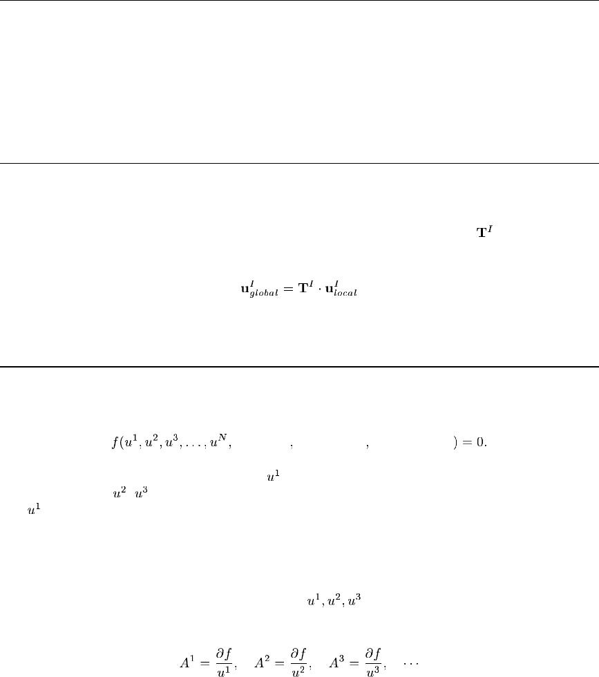
MPC
Constraints that involve degrees of freedom that are not active in the model
The degrees of freedom involved in user M PCs must appear on some elem ent or Abaqus/Standard MPC
type in the m odel: user MPCs cannot use degrees of freedom that have not been introduced somewhere
on an element. For example, a mesh that uses only continuum (solid) elements cannot have user MPCs
that involve rotational degrees of freedom. The simplest way to overcome this limitation is to introduce
an element somewhere in the model that uses the required degrees of freedom but does not affect the
solution in any other way. Alternatively, if the degrees of freedom are rotations, they can be activated by
the use of a library BEAM-type MPC somewhere in the m odel.
Use with nodal coordinate systems
When a local coordinate system (“Transforme d coordina te syst ems,” Section 2.1.5 of the Abaqus
Analysis User’s Manual) and a user MPC are both used at a node, the variables at the node are
first transformed before the MPC is imposed. Therefore, user-supplied MPCs m ust be based on the
transformed degrees of freedom. The local-to-global transformation matrices
for the individual
nodes:
are passed in for information.
Degree of freedom version of user subroutine MPC
This version of user subroutine MPC allows for one individual degree of freedom to be constrained and,
thus, eliminated at a time . The constraint can be quite general and nonlinear of the form:
geometry temperature field varia bles
The first degree of freedom in this function, , is the degree of freedom that will be elim inated to im pose
the constraint.
, , etc. are any other degrees of freedom that ar e involved in the cons traint. Since
will be eliminated to impose the constraint, it cannot be used in subsequent kinematic constraints
(multi-point constraints, linear equation constraints, or boundary conditions). Therefore, the user MPCs
are imposed in the order given in the input.
You must provide, at all times, two item s of information in user subroutine MPC:
1. A list of degree of freedom identifiers at the nodes that are listed in the c orresponding multi-point
constraint definition. This l ist corresponds to
, etc. in the constraint as given above.
2. An array of the derivatives
1.1.14–2
Abaqus ID:
Printed on:

MPC
of the constraint function with respect to the degrees of freedom involved. This array is needed for
the redistribution of loads from degree of freedom
to the other degrees of freedom and for the
elimination of
from the system matrices.
In addition, you can provide the value of the dependent degre e of freedom
as a function of
the independent degrees of freedom
etc. If this value is not provided, Abaqus/Standard will
update
based on the linearized form of the constraint equation as
Subroutine MPC should be coded and checked with care: if the array of derivatives , etc. does
not correspond to the definition of
in terms of , , etc., forces will be transmitted improperly
by the MPC and violations of equilibrium may occur. In addition, convergence of the solution may
be adversely affected.
User subroutine interface
SUBROUTINE MPC(UE,A,JDOF,MDOF,N,JTYPE,X,U,UINIT,MAXDOF,
* LMPC,KSTEP,KINC,TIME,NT,NF,TEMP,FIELD,LTRAN,TRAN)
C
INCLUDE 'ABA_PARAM.INC'
C
DIMENSION A(N),JDOF(N),X(6,N),U(MAXDOF,N),UINIT(MAXDOF,N),
* TIME(2),TEMP(NT,N),FIELD(NF,NT,N),LTRAN(N),TRAN(3,3,N)
user coding to define UE, A, JDOF, and, optionally, LMPC
RETURN
END
Variables to be defined
A(N)
An array containing the derivatives of the constraint func tion,
The coding in the subroutine mus t define N entries in A,whereN is defined below.
1.1.14–3
Abaqus ID:
Printed on:

MPC
JDOF(N)
An array containing the degree of freedom identifiers at the nodes that are involved in the constraint.
For example, if
is the z-displacement at a node, give JDOF(1) = 3; if is the x-displacem ent at
a node, give JDOF(2) = 1. The codi ng in the subroutine must define N e ntries in JDOF,whereN is
defined below.
Variables that can be updated
UE
This variable is passed in as the total value of the eliminated degree of freedom,
. This variable will
either be zero or have the current value of
based on the linearized constraint equation, depending at
which stage of the iteration the user subroutine is called. If the constraint is linear and is used in a small-
displacement analysis (nonlinear geometric effects are not considered) or in a perturbation analysis, this
variable need not be defined: Abaqus/Standard will compute
as
If the constraint is nonlinear, this variable should be updated to the value of at the end of the
increment to satisfy the constraint exactly. If the return value is the same as the incoming value,
Abaqus/Standard w ill update the eliminated degree of freedom based on the linearized form of the
constraint equation. In this case the constraint is not likely to be satisfied exactly.
LMPC
Set this variable to zero to avoid the application of the multi-poi nt constraint. The MPC will be applied
if the variable is not changed. This variabl e must be set to zero e very time the subroutine is c alled if
the user MPC is to remain deactivated. This MPC variable is useful for switching the MPC on and off
during an analysis. However, the option should be used with care: switching off an MPC may cause
a sudden disturbance in equilibri um, which can lead to conve rgence problems. If this variable is used
to switch on an MPC during an analysis, the variable UE should be defined; otherw ise, the constraint
may not be satisfied properly.
Variables passed in for information
MDOF
Maximum number of active degre es of freedom per node involved in the MPC. For th e degre e of
freedom mode of user subroutine MPC, MDOF=1.
N
Number of degrees of freedom that are involved in the constraint, defined as the number of nodes given
in the corresponding multi-point constraint definition. If more than one degree of freedom at a node is
1.1.14–4
Abaqus ID:
Printed on:
MPC
involved in a constraint, the node m ust be repeated as needed or, alternatively, the nodal mode should
be used.
JTYPE
Constraint identifier given for the corresponding m ulti-point constraint definition.
X(6,N)
An array containing the original coordinates of the nodes involved in the constraint.
U(MAXDOF,N)
An array containing the values of the degrees of freedom at the nodes involved in the constraint. These
values will be either the values at the end of the previous iteration or the current values based on the
linearized constraint equation, depending at which stage of the iteration the user subroutine is called.
UINIT(MAXDOF,N)
An array containing the values at the beginning of the current iteration of the degrees of freedom at the
nodes involved in the constraint. This information is useful for decision- making purposes when you do
not want the outcome of a decision to change during the course of an it eration. For example, there are
constraints in which the degree of freedom to be eliminated changes during the course of the analysis,
but it is necessary to prevent the choice of the depe ndent degree of freedom from changing during the
course of an iteration.
MAXDOF
Maximum degree of freedom num ber at any node in the analysis. For example, for a coupled
temperature-displacement analysis with continuum elements, MAXDOF will be equal to 11.
KSTEP
Step number.
KINC
Increment number within the step.
TIME(1)
Current value of step time.
TIME(2)
Current value of total time.
NT
Number of positions through a section where temperature or field variable values are stored at a node.
In a mesh containing only continuum elements, NT=1. For a mesh containing shell or beam elements,
NT is the largest of the values specified for the numbe r of temperature points in the s hell or beam section
definition (or 2 for temperatures specified together with gra dients for shells or two-dimensional beams,
3 for temperatures specified together with gradients for three-dimensional beams).
1.1.14–5
Abaqus ID:
Printed on:

MPC
NF
Number of different predefined field variables requested for any node (including field variables defined
as initial conditions).
TEMP(NT,N)
An array containing the tem peratures at the nodes involved in the constraint. This array is not used
for a heat transfer, coupled temperature-displacement, or coupled therm al-electrical analysis since the
temperatures are degrees of freedom of the problem.
FIELD(NF,NT,N)
An array containing a ll field variables at the nodes involved in the constraint.
LTRAN(N)
An integer array indicating whether the nodes in the MPC are transformed. If LTRAN(I)=1,a
transformation is applied to node I;ifLTRAN(I)=0,notransformationisapplied.
TRAN(3,3,N)
An array containing the local-to-global transformation matrices for the nodes used in the MPC. If no
transformation is present at node I, TRAN(*,*,I) is the identity matrix.
Example: Nonlinear single degree of freedom MPC
An example of a nonlinear single degree of freedom MPC is a geometrically nonlinear two-dimensional
slider involving nodes a, b,andc. The constraint forces node a to be on the straight line connecting
nodes b and c (see Figure 1.1.14–1).
b
a
c
y
x
Figure 1.1.14–1 Nonlinear MPC exam ple: two-dimensional slider.
1.1.14–6
Abaqus ID:
Printed on:

MPC
The constraint equation can be written in the form
where , ,and are the current locations of a, b,andc. The derivatives are readily
obtained as
Depending on the orientation of the segment we choose either or as the degree of freedom
to be eliminated. If
, we choose as the dependent degree of freedom. If
, we choose as the dependent degree of freedom . Moreover, if points b and c
are coincident, the constraint is not applied.
To prevent the choice of either
or as the dependent degre e of freedom from changing during
the course of an iteration, the orientation of the segment
is tested based on the geometry at the
beginning of the iteration. The dependent degree of freedom is allowed to change from increment to
increment.
Suppose the above multi-point constraint is defined as type 1, with nodes a, a, b, b, c, c. The user
subroutine MPC could be coded as follows:
SUBROUTINE MPC(UE,A,JDOF,MDOF,N,JTYPE,X,U,UINIT,MAXDOF,
* LMPC,KSTEP,KINC,TIME,NT,NF,TEMP,FIELD,LTRAN,TRAN)
C
INCLUDE 'ABA_PARAM.INC'
C
DIMENSION A(N),JDOF(N),X(6,N),U(MAXDOF,N),UINIT(MAXDOF,N),
* TIME(2),TEMP(NT,N),FIELD(NF,NT,N),LTRAN(N),TRAN(3,3,N)
PARAMETER( PRECIS = 1.D-15 )
C
IF (JTYPE .EQ. 1) THEN
DYBC0 = X(2,5) + UINIT(2,5) - X(2,3) - UINIT(2,3)
DXBC0 = X(1,3) + UINIT(1,3) - X(1,5) - UINIT(1,5)
DYBC = X(2,5) + U(2,5) - X(2,3) - U(2,3)
DXBC = X(1,3) + U(1,3) - X(1,5) - U(1,5)
A(3) = X(2,1) + U(2,1) - X(2,5) - U(2,5)
A(4) = X(1,5) + U(1,5) - X(1,1) - U(1,1)
A(5) = X(2,3) + U(2,3) - X(2,1) - U(2,1)
A(6) = X(1,1) + U(1,1) - X(1,3) - U(1,3)
JDOF(3) = 1
1.1.14–7
Abaqus ID:
Printed on:

MPC
JDOF(4) = 2
JDOF(5) = 1
JDOF(6) = 2
IF (ABS(DYBC0).LE.PRECIS .AND. ABS(DXBC0).LE.PRECIS) THEN
C
C POINTS B AND C HAVE COLLAPSED. DO NOT APPLY CONSTRAINT.
C
LMPC = 0
ELSE IF (ABS(DXBC0) .LT. ABS(DYBC0)) THEN
C
C MAKE U_A DEPENDENT DOF.
C
JDOF(1) = 1
JDOF(2) = 2
A(1) = DYBC
A(2) = DXBC
UE = A(5)A(2)/A(1) + X(1,3) + U(1,3) - X(1,1)
ELSE
C
C MAKE V_A DEPENDENT DOF.
C
JDOF(1) = 2
JDOF(2) = 1
A(1) = DXBC
A(2) = DYBC
UE = -A(6)A(2)/A(1) + X(2,3) + U(2,3) - X(2,1)
END IF
END IF
C
RETURN
END
Nodal version of user subroutine MPC
The nodal vers ion of user su broutine MPC allows for m ultiple degrees of freedom of a node to be
eliminated sim ultaneously. The set of constraints can be quite general and nonlinear, of the form
geometry temperature field variables
NDEP is the number of dependent degrees of freedom that are involved in the constraint and should
have a value between 1 and MDOF, w hich is the number of active degrees of freedom per node in the
analysis. N is the number of nodes involved in the constraint. The scalar co nstraint functions
can also
1.1.14–8
Abaqus ID:
Printed on:

MPC
be considered as a vector function , and the first set of degrees of freedom in the vector function
will be eliminated to impose the constraint. The sets , , etc. are the independent degrees of
freedom at nodes 2, 3, etc. involved in the constraint. The set
must be composed of NDEP degrees of
freedom at the first node of the MPC definition. For example, if the dependent degrees of freedom are
the x-displacement, the z-displacement, and the y-r otation at the first node,
. ,
etc. can be composed of any num ber of degrees of freedom, depending on which ones play a role in the
constraint, and need not be of the same size; for example,
and .
The dependent node can also reappear as an independent node in the MPC. However, since the
dependent degrees of freedom of th is node will be el iminated, they cannot be use d as indepen dent
degrees of freedom in this MPC. For example, if the rotations at node a are constrained by the MPC,
the displacements of node a can still be used as inde pendent degrees of freedom in the MPC, but the
rotations them selves cannot. Similarly, the degrees of freedom that will be eliminated to impose the
constraint cannot be used in subsequent kinematic constraints (multi-point constraints, linear equation
constraints, or boundary conditions). The MPCs are impose d in the order given in the input for this
purpose.
The nodal version of user subroutine MPC was designed with the application of nonlinear
constraints involving large three-dimensional rotations in m ind. D ue to the increm ental nature of the
solution procedure in Abaqus/Standard, a linearized set of constraints
where , , etc. is applied during each iteration. This
linearized set of constraints is used for the calculation of equilibrium. For finite rotations the linearized
equation is given in terms of the linearized rotations
, , ,…,yielding
Since the linearized rotation field, , is not the varia tion of the total rotation vector, (see “Rotation
variables,” Sec tion 1.3.1 of the Abaqus Theory Manual), you cannot obta in the linearized constraint
equation by simply taking derivatives of the vector function,
, with respect to the rotational degrees
of freedom involved. The formulation of the linearized constraint in
is equivalent to the formulat ion
of a geometrically linear constraint in the deformed configuration and is generally easier to formulate
than the const raint in terms of
. For an exact formulation of the constraint, the dependent compon ents
of the total rotation vector
must be defined exactly (see “Rotation variables,” Section 1.3.1 of the
Abaqus Theory Manual).
You must provide, at all times, two items of information in subroutine MPC:
1. A matrix of degree of freedom identifiers at the nodes that are listed in the corresponding m ulti-
point constraint definition. The columns of this m atrix correspond to
,etc.inthesetof
constraints as given above, w here unused entries are padded with zeros. The number of nonzero
entries in
will implicitly determine the number of dependent degrees of freedom, NDEP.
2. The matrices representing the linearized constraint function w ith respect to the degrees of freedom
involved. These m atrices are needed for the redistribution of loads from degrees of freedom
to
1.1.14–9
Abaqus ID:
Printed on:

MPC
the other degrees of freedom and for the elimination of from the system m atrices. For constraints
that do not involve three-dimensional rotations and constraints with planar rotations, t hese matrices
can be readily obtained from the derivatives of the total constraint function with respect to the
degrees of freedom involved:
For constraints that involve finite r otations, the matrices follow from the linearized form:
In addition, you can provide the values of the dependent degrees of freedom , as a functi on of
the independent degrees of freedom
etc. For finite rotations, must be specified as a
function of
, , etc. If thes e values are not provided, Abaqus/Standard will update based on
the linearized form of the constraint equations. Subroutine MPC should be coded and checked with
care: if the m atrices of derivatives
, etc. do not correspond to the definit ion of in terms of
, etc., forces will be transmitted improperly by the MPC and violations of equilibrium may
occur. In addition, convergence of the solution may be adversely affected.
User subroutine interface
SUBROUTINE MPC(UE,A,JDOF,MDOF,N,JTYPE,X,U,UINIT,MAXDOF,
* LMPC,KSTEP,KINC,TIME,NT,NF,TEMP,FIELD,LTRAN,TRAN)
C
INCLUDE 'ABA_PARAM.INC'
C
DIMENSION UE(MDOF),A(MDOF,MDOF,N),JDOF(MDOF,N),X(6,N),
* U(MAXDOF,N),UINIT(MAXDOF,N),TIME(2),TEMP(NT,N),
* FIELD(NF,NT,N),LTRAN(N),TRAN(3,3,N)
user coding to define JDOF, UE, A and, optionally, LMPC
RETURN
END
1.1.14–10
Abaqus ID:
Printed on:

MPC
Variables to be defined
JDOF(MDOF,N)
Matrix of degrees of freedom identifiers at the nodes involved in the constraint. Before each call to
MPC, Abaqus/Standard will initialize all of the entries of JDOF to zero. All active degrees of freedom
for a given column (first index ranging from 1 to MDOF) must be defined starting at the top of the
column with no zeros in between. A zero will mark the end of the list for that column. The number
of nonzero entries in the first column will implicitly determine the numbe r of dependent degrees of
freedom (NDEP). For example, if the dependent degrees of freedom are the z-displacement, the x-
rotation, and the z-rotation at the firs t node, NDEP
and
If the degrees of freedom at the third node involved in the MPC are the x-displacem ent and the y-
rotation, define
A(MDOF,MDOF,N)
Submatrices of coefficients of the linearized constraint function,
Before each call to user subroutine MPC, Abaqus/Standard will initialize all of the entries of A to zero;
therefore, only nonzero entries need to be defined. If the coding in the subroutine defines NDEP nonzero
entries in the column JDOF(J,1), it should de fine NDEP × NDEP entries in the s ubmatrix A(I,J,1).
Since this submatrix will be inverted to impose the MPC, it must be nonsingular. A maximum of NDEP
× MDOF entries can be defined for the remaining submatrices A(I,J,K), K=2,
, N. The number
of columns in each submatrix A(I,J,K) must correspond to the number of nonzero entries in the
corresponding column of the matrix JDOF(J,K).
Variables that can be updated
UE(NDEP)
This array is passed in as the total value of the eliminated degrees of freedom ,
.Thisarray
will either be zero or contain the current values of
based on the linearized constraint equations,
depending at w hich stage of the iteration the user subroutine is called. For small-displacement analysis
or perturbation analysis this array need not be defined: Abaqus/Standard will com p ute
as
1.1.14–11
Abaqus ID:
Printed on:

MPC
For large-displacement analysis this array can be updated to the value of at the end of the
increment to satisfy the constraint exactly. If the return values are the same as the incoming values,
Abaqus/Standard will update the elim inated degrees of freedom based on the linearized form of the
constraint equations. In this case the constraint is not likely to be satisfied exactly.
LMPC
Set this variable to zero to avoid the application of the multi-point constraint. If the variable is not
changed, the MPC will be applied. This variable must be set to zero every time the subroutine is called
if the user M PC is to remain deactivated. This MPC variable is useful for switching the MPC on and off
during an analysis. This option should be used with care: switching off an MPC may cause a sudden
disturbance in equilibrium, which can lead to convergence problems.
Variables passed in for information
MDOF
Number of active degrees of freedom per node in the analysis. For example, for a coupled tem perature-
displacement analysis with two-dimensional continuum elements, the active degrees of freedom are 1,
2, and 11 and, hence, MDOF will be equal to 3.
N
Number of nodes involved in the constraint. The value of N is defined as the number of nodes given in
the corresponding multi-point constraint definition .
JTYPE
Constraint identifier given for the corresponding m ulti-point constraint definition.
X(6,N)
An array containing the original coordinates of the nodes involved in the constraint.
U(MAXDOF,N)
An array containing the values of the degrees of freedom at the nodes involved in the constraint. These
values will either be the values at the end of the previous iteration or the current values based on the
linearized constraint equation, depending at which stage of the iteration the user subroutine is called.
UINIT(MAXDOF,N)
An array containing the values at the beginning of the curr ent iteration of the degrees of freedom at
the nodes involved in the constraint. This information is useful for decision-ma king purposes when
you do not want the outcome of a decision to change during the course of an iteration . For example,
there are constraints in which the degrees of freedom to be eliminated change during the course of the
analysis, but it is necessary to prevent the choice of the dependent degrees of freedom from changing
during the course of an iteration.
1.1.14–12
Abaqus ID:
Printed on:
MPC
MAXDOF
Maximum degree of freedom num ber at any node in the analysis. For example, for a coupled
temperature-displacement analysis with continuum elem ents, MAXDOF is equal to 11.
KSTEP
Step number.
KINC
Increment number within the step.
TIME(1)
Current value of step time.
TIME(2)
Current value of total time.
NT
Number of positions through a section where temperature or field variable values are stored at a node.
In a mesh containing only continuum elements, NT=1. For a mesh containing shell or beam elements,
NT is the largest of the values specified for the numbe r of temperature points in the s hell or beam section
definition (or 2 for temperatures specified together with gra dients for shells or two-dimensional beams,
3 for temperatures specified together with gradients for three-dimensional beams).
NF
Number of different predefined field variables requested for any node (including field variables defined
as initial conditions).
TEMP(NT,N)
An array containing the tem peratures at the nodes involved in the constraint. This array is not used
for a heat transfer, coupled temperature-displacement, or coupled therm al-electrical analysis since the
temperatures are degrees of freedom of the problem.
FIELD(NF,NT,N)
An array containing a ll field variables at the nodes involved in the constraint.
LTRAN(N)
An integer array indicating whether the nodes in the MPC are transformed. If LTRAN(I)=1,a
transformation is applied to node I;ifLTRAN(I)=0,notransformationisapplied.
TRAN(3,3,N)
An array containing the local-to-global transformation matrices for the nodes used in the MPC. If no
transformation is present at node I, TRAN(*,*,I) is the identity matrix.
1.1.14–13
Abaqus ID:
Printed on:

MPC
Example: Nonlinear MPC
As an example of a nonlinear MPC, consider the insertion of a rigid beam in a large-displacement, planar
(two-dimensional) problem. This MPC is the two-dimensional version of library BEAM-type MPC. It
can be implemented as a set of three different single degree of freedom MPCs or as a single nodal MPC.
Here, the second method will be worked out because it is simpler and requires less data input.
Let a and b (see Figure 1.1.14–2) be the ends of the beam, with a the dependent end.
y
x
L
b
φ
z
b
+ φ
0
a
Figure 1.1.14–2 Nonlinear MPC exam ple: rigid beam .
The rigid beam will then define both components of displacement and the rotation at a in terms of
the displacements and rotation at end b according to the set o f equations:
where and , and are the current locations of a and
b,
and are the rotations at a and b about th e z-axis, L is the length of the link, and is the original
orientation of the link.
In terms of the original positions
and of a and b,
and
where and . Thus, the constraint equations can be expressed as
1.1.14–14
Abaqus ID:
Printed on:

MPC
In light of the above fo rmulation, the nontrivial portions of the mat rices A and JDOF are
and
Since degree of freedom 6 ( ) appears in this constraint, there must be an elem ent in the mesh that uses
that degree of freedom —a B21 beam elem ent, for exam ple.
If the above multi-point constra int is defined as type 1 with nodes a and b, the user subroutine MPC
could be coded as follows:
SUBROUTINE MPC(UE,A,JDOF,MDOF,N,JTYPE,X,U,UINIT,MAXDOF,LMPC,
* KSTEP,KINC,TIME,NT,NF,TEMP,FIELD,LTRAN,TRAN)
C
INCLUDE 'ABA_PARAM.INC'
C
DIMENSION UE(MDOF),A(MDOF,MDOF,N),JDOF(MDOF,N),X(6,N),
* U(MAXDOF,N),UINIT(MAXDOF,N),TIME(2),TEMP(NT,N),
* FIELD(NF,NT,N),LTRAN(N),TRAN(3,3,N)
C
IF (JTYPE .EQ. 1) THEN
COSFIB = COS(U(6,2))
SINFIB = SIN(U(6,2))
ALX = X(1,1) - X(1,2)
ALY = X(2,1) - X(2,2)
C
UE(1) = U(1,2) + ALX*(COSFIB-1.) - ALY*SINFIB
UE(2) = U(2,2) + ALY*(COSFIB-1.) + ALX*SINFIB
UE(3) = U(6,2)
C
A(1,1,1) = 1.
A(2,2,1) = 1.
A(3,3,1) = 1.
1.1.14–15
Abaqus ID:
Printed on:

MPC
A(1,1,2) = -1.
A(1,3,2) = ALX*SINFIB + ALY*COSFIB
A(2,2,2) = -1.
A(2,3,2) = -ALX*COSFIB + ALY*SINFIB
A(3,3,2) = -1.
C
JDOF(1,1) = 1
JDOF(2,1) = 2
JDOF(3,1) = 6
JDOF(1,2) = 1
JDOF(2,2) = 2
JDOF(3,2) = 6
END IF
C
RETURN
END
Example: Nonlinear MPC involving finite rotations
As an example of a nonlinear MPC involving finite rotations, consider a two-dimensional constant
velocity joint that might be part of a robotics application. Let a, b, c (see Figure 1.1.14–3) be the nodes
making up the joint, with a th e dependent node.
x
y
a
bc
φ
b
φ
c
Figure 1.1.14–3 Nonlinear MPC example: constant velocity joint.
The joint is operated by prescribing an axial rotation
at c and an out-of-plane rotation
at b. The compounding of these two prescribed rotation fields will determine the tota l rotation at
a. We can form ally write this constraint as follows:
1.1.14–16
Abaqus ID:
Printed on:

MPC
where denotes the rotation product. The formulation of the linearized constraint can be readily achieved
from geom etrically linear considerations in the deformed state.
In geometrically linear pr oblems compound rotations are obtained sim ply as the linear superposition
of individual rotation vectors. Consider the geometry depicte d in Figure 1.1.14–3 and assume that the
infinitesimal rotations
and are applied at c and b, respectively. The rotation
at a will simply be the sum of the vector to the vector rotated by an angle about the
z-axis. Thus, the linearized constraint can be w ritten directly as
In light of this formula tion, the nontrivial portions of the matrices JDOF and A are
and
Since degrees of freedom 4 ( ), 5( ), and 6( ) appear in this constraint, there must be an element
in the mesh that uses these degrees of freedom—a B31 beam element, for exam ple. The MPC subroutine
has been coded with just this information. In this case Abaqus/Standard updates the dependent rotation
field,
, based on the linearized constraint equations. Although the constraint is not satisfied exactly,
good results are obtained as long as the rotation increments are ke pt small enough. A more rigorous
derivation of the linearized constraint and the exact nonlinear recovery of the dependent degrees of
freedom is presented in “Rotation variables,” Section 1.3.1 of the Abaqus Theory Manual.
If the above multi-point constraint is defined as type 1 with nodes a, b,andc, user subroutine MPC
could be coded as follows:
SUBROUTINE MPC(UE,A,JDOF,MDOF,N,JTYPE,X,U,UINIT,MAXDOF,LMPC,
* KSTEP,KINC,TIME,NT,NF,TEMP,FIELD,LTRAN,TRAN)
C
INCLUDE 'ABA_PARAM.INC'
C
DIMENSION UE(MDOF),A(MDOF,MDOF,N),JDOF(MDOF,N),X(6,N),
* U(MAXDOF,N),UINIT(MAXDOF,N),TIME(2),TEMP(NT,N),
1.1.14–17
Abaqus ID:
Printed on:
MPC
* FIELD(NF,NT,N),LTRAN(N),TRAN(3,3,N)
C
IF (JTYPE .EQ. 1) THEN
A(1,1,1) = 1.
A(2,2,1) = 1.
A(3,3,1) = 1.
A(3,1,2) = -1.
A(1,1,3) = -COS(U(6,2))
A(2,1,3) = -SIN(U(6,2))
C
JDOF(1,1) = 4
JDOF(2,1) = 5
JDOF(3,1) = 6
JDOF(1,2) = 6
JDOF(1,3) = 4
END IF
C
RETURN
END
1.1.14–18
Abaqus ID:
Printed on:

ORIENT
1.1.15 ORIENT: User subroutine to provide an orientation for defining local material
directions or local directions for kinematic coupling constraints or local rigid body
directions for inertia relief.
Product:
Abaqus/Standard
References
•
“Orientations,” Section 2.2.5 of the Abaqus Analysis User’s Manual
• *
ORIENTATION
•
“Eigenvalue analysis of a piezoelectric transducer,” Section 7.1.1 of the Abaqus Example Problems
Manual
Overview
User subroutine ORIENT:
•
will be called at the start of the analysis at each location (m aterial point, special-purpose element,
coupling node, or reference point for inertia relief) for which local directions are defined with a
user-subroutine-defined orientation;
•
is used to code the direction cosines of a preferred local material orient ation, for which anisotropic
or orthotropic material properties have been defi ned or for which stress output is desired, in t erms
of the normal ( nonoriented) material basis directi ons;
•
can be used to define the direction cosines orienting the layer of reinforcing material in membrane,
shell, or surface elements (see “Defining reinforcement,” Section 2.2.3 of the A baqus A nalysis
User’s Manual);
•
can be used to provide a local system for defining the direction of action of rotary inertia, spring,
dashpot, flexible joint, and elastic-plastic joint elements;
•
can be used with gasket elements to define the local in-plane directions for three-dimensional area
and three-dimensiona l link elements that consider transverse shear and membrane deformations
(see “Defining the gasket behavior directly using a gasket behavior m odel,” Section 29.6.6 of the
Abaqus Analysis User’s Manual);
•
can be used to define a local system in which coupling constraints are applied (see “Co upling
constraints,” Section 31.3.2 of the Abaqus Analysis User’s Manual, and “Kinematic coupling
constraints,” Section 31.2.3 of the Abaqus Analysis User’s Manual);
•
can be used to define a local system at the reference point for the rigid body directions in which
inertia relief loads are applied for the entire m odel (see “Inertia relief,” Section 11.1.1 of the Abaqus
Analysis User’s Manual);
•
interprets “defa ult basis directions” as the global directions for continuum elements and as the
default surface directions for shell, m embrane, and surface elem ents (as described in “Conventions,”
Section 1.2.2 of the Abaqus Analysis User’s Manual); and
1.1.15–1
Abaqus ID:
Printed on:

ORIENT
•
ignores any data specified for the associated or ientation definition outside the user subroutine.
The local directions defined by user subroutine ORIENT m ust be specified relative to the default basis
directions.
User subroutine interface
SUBROUTINE ORIENT(T,NOEL,NPT,LAYER,KSPT,COORDS,BASIS,
1 ORNAME,NNODES,CNODES,JNNUM)
C
INCLUDE 'ABA_PARAM.INC'
C
CHARACTER*80 ORNAME
C
DIMENSION T(3,3),COORDS(3),BASIS(3,3),CNODES(3,NNODES)
DIMENSION JNNUM(NNODES)
user coding to define T
RETURN
END
Variable to be defined
T
An array containing the direction cosines of the preferred orientation in terms of the default basis
directions. T(1,1), T(2,1), T(3,1) give the (1, 2, 3) components of the first direction; T(1,2),
T(2,2), T(3,2) give the second direction; etc. For shell and membrane elements only the first
and second directions are used. The directions do not have to be normalized. If the second direction
is not orthogonal to the first direc tion, Abaqus/Standard will orthogonaliz e and normalize the second
direction with respect to the first. The third direction is then determined by taking the cross product of
the first and second directions. For planar elem ents the first two directions must lie in the plane of the
element.
For use with coupling constraints (“ Coupling constraints,” Section 31.3.2 of the Aba qus Analysis
User’s Manual), the local basis directions are used as the local constraint directions for application of
the kinematic constraint.
For use with inertia relief loads, the local basis directions are used as the rigid body direction
vectors for computing the loads.
Variables passed in for information
NOEL
Element number. This value is ze ro when the subroutine is called for use with coupling constraints or
inertia relief loads.
1.1.15–2
Abaqus ID:
Printed on:
ORIENT
NPT
Integration point number. This variable is set only for relevant uses.
LAYER
Layer number (for composite shells and layered solids). This variable is set only when relevant. It
is equal to zero when it is irrelevant, such as in a regular solid element or in a shell elem ent when
transverse shear stiffness calculations are performed.
KSPT
Section point number within the current layer. This variable is set only when relevant. It is equal to
zero when it is irrelevant, such as in a regular solid element or in a shell element when transverse shear
stiffness calculations are performed.
COORDS
An array containing the initial coordinates of this point. This array contains the coordinates of the
reference point for inertia relief loads.
BASIS
An array containing the direction cosines of the normal material basis directions in terms of the global
coordinates in the original configuration. BASIS(1,1), BASIS(2,1), BASIS(3,1) give the 1-
direction, etc. This is useful only in shells or m embranes since in all other cases the basis is the global
coordinate system.
ORNAME
User-specified orientation name, left justified, with one exception. When an overall section orientation
is specified for a composite solid or shell section and the individual layer orientations are specified by
an orientation angle, Abaqus defines an internal orientation name to represent the actual orientation of
the layer. To avoid internal names, provide an orientation name rather than an orien tation angle as part
of the layer definition for each individual layer of a composite section.
NNODES
Number of element nodes. This value i s two when the subroutine is called for us e with a kinematic
coupling definition, where the two nodes are the reference and current coupling node. When used with
a distributing coupling definition, this number is equal to the number of coupling nodes plus one for
the reference node. It is one when used with inertia relief loads since the local basis is defined at the
reference point.
CNODES
An array containing the original coordinates of the nodes. When used with a kinematic coupling
definition, the first entry defines the reference node coordinates, and the second entry defines the
coupling node coordinates. When used with a distributing coupling definition, the first entry defines
the reference node coordinates, and the subsequent entries define the coupling node coordinates in the
order defined by the JNNUM array. When used with inertia relief loads, this array is not used. For all
other uses the entry order follows that of the element definition node ordering.
1.1.15–3
Abaqus ID:
Printed on:
ORIENT
JNNUM
An array containing the NNODES node num bers. When used with a kinematic coupling definition,
the first entry is the reference nod e number, and the second entry i s the node number for the current
coupling node. When used with a distributing coupling definition, the first entry is the reference node
number followed by the node numbers of all coupling nodes. Wh en used with inertia relief loads, this
array is not used. For all other uses the entry order follows that of the element definition node ordering.
1.1.15–4
Abaqus ID:
Printed on:

RSURFU
1.1.16 RSURFU: User subroutine to define a rigid surface.
Product:
Abaqus/Standard
References
•
“Analytical rigid surface definition,” Section 2.3.4 of the Abaqus Analysis User’s Manual
• *
SURFACE
• *
RIGID BODY
•
“RSURFU,” Section 4.1.10 of the A baqus Verification Manual
Overview
User subroutine RSURFU:
•
is used to define the surface of a rigid body for use in contact pairs;
•
can be used to define a complex rigid surface if the various capabilities provided for defining a
surface in Abaqus (see “Analytical rigid surface definition,” Section 2.3.4 of the Abaqus Analysis
User’s Manual) are too restrictive;
•
will be called at points on the slave surface of a contact pair or, if contact elements are used, at each
integration point of each contact element with which the rigid surface is associated; and
•
requires the definition of the closest point on the rigid surface, the normal and tangent directions,
and the surface curvature.
Overpenetration constraint
This routine must determine if a point on the slave surface has penetrated the rigid surface and define the
local surface geometry. If the deforming and rigid surfaces are in contact at this point, Abaqus/Standard
will impose a constraint at the point to prevent overpenetration. The local surface geom etry must be
defined to provide the necessary orientation for the constraint equations and friction directions and to
allow Abaqus/Standard to compute the rate of change of these equations as the point moves around on
the surface—the “tangent stiffness m atrix” for the surface in the Newton algorithm. For the purpose
of these calculations, it is best to define a smooth surface. If the surface is defined in a discontinuous
manner, convergence may be adversely affected.
Calculations to be performed
Each time RSURFU is called, Abaqus /Standard give s the current position of point A on the surface
of the deforming structure,
; the current position of the rigid body reference point, ; the total
displacements of both of these points,
and ; and the total rotation of the rigid body reference
point,
.
The routine should perform the following calculations:
1.1.16–1
Abaqus ID:
Printed on:

RSURFU
1. A point, A′, must be found on the rigid surface at which the normal to the surface passes through
. If there is not a unique point A′, the routine must choose the most suitable point (usually the
closest A′ to A). The routine must pass back the coordinates of A′ to Abaqus/Standard. For the
surface-to-surface contact formulation, the slave normal, not the master normal, should be used.
2. RSURFU must define the distance, h,bywhichA has penetrated the surface below A′. A ne gative
value of h means that A is outside the surface of the rigid body.
3. If the surfaces are in contact, which may sometim es be the case even if h is negative, RSURFU must
define the local surface geometry.
Defining the local surface geometry
There are two scenarios under which it is mandatory that the routine define the local surface geometry:
if A has penetrated the surface—
if the surface behavior is truly rigid, or h is greater than the
maximum overclosure value specified for m odified surface behavior using either contact controls (see
“Adjusting contact controls in Abaqus/Standard,” Section 32.3.6 of the Abaqus Analysis User’s Manual)
or a modified pr essure-overclosure relationship (see “Contact pressu re-overclosure r elationships,”
Section 33.1.2 of the Abaqus Analysis User’s Manual)—and if A was in contact at the beginning of the
increment, in which case the flag LCLOSE=1 (see the variable list for the definition of LCLOSE). The
variable LCLOSE is not relevant for the surface-to-surface contact form ulation and is always passed in
as 0. The routine can be coded so that local surface geometry definitions are always provided regardless
of the scenario.
The local surface geometry is specified by two orthogonal tangents to the rigid surface at A′, as well
as the rates of change of th e outward pointing normal at A′,
, with respect to local surface coordinates
that are distance measuring along the tang ents,
and (see Figure 1.1.16–1).
n
A
A
t
S
t
S
1
2
2
1
Figure 1.1.16–1 Local geom etry on a rigid surface.
The tangents to the surface at A′ must be defined so that their positive, right-handed cross product is
the outward normal to the surface. For two-dimensional cases Abaqus/Standard assum es that the second
tangent is (0, 0, −1), so that when you give the direction cosines of the first tangent as (
, , 0), the
1.1.16–2
Abaqus ID:
Printed on:

RSURFU
outwardnormalwillbe( , , 0 ). The rates of change of the normal with respect to and are
required to define the local curvature of the surface.
User subroutine interface
SUBROUTINE RSURFU(H,P,TGT,DNDS,X,TIME,U,CINAME,SLNAME,
1 MSNAME,NOEL,NODE,LCLOSE)
C
INCLUDE 'ABA_PARAM.INC'
C
CHARACTER*80 CINAME,SLNAME,MSNAME
C
DIMENSION P(3),TGT(3,2),DNDS(3,2),X(3,3),TIME(2),U(6,2)
user coding to define H, P, TGT, and DNDS
RETURN
END
Variables to be defined
H
Penetration of the point A on the deform ing structure into the surface of the rigid body, measured
down the outward normal to the rigid surface. A negative value of H indicates that A is outside the
rigid surface. Even for a com pletely rigid surface, A may appear to penetrate the surface duri ng the
iterations because the kinematic constraints are not fully satisfied until an increment converges.
P(3)
Position of the point A′ on the surface of the rigid body closest to point A on the surface of t he deforming
structure.
TGT(3,2)
Direction cosines of the two unit tangents to the surface,
and , at point A′. For two-dimensio nal
cases only the first two components of
need be given since in this case A baqus/Standard assum es
that
is(0,0,−1).
DNDS(3,2)
Rates of change of the surface normal,
,atA′, w ith respect to distance measuring coordinates, and
,along and . For two-dimensional cas es only the first two en tries in the first column of DNDS
(
, ) are required. The array DNDS is not required to be assigned for the surface-to-
surface contact formulation.
1.1.16–3
Abaqus ID:
Printed on:

RSURFU
Variables passed in for information
X(K1,1)
Current coordinates of point A on the surface of the deforming structure.
X(K1,2)
Current coordinates of the rigid body re ference point.
X(K1,3)
Unit normal vector for point A; relevant only for the surface-to-surface contact formulation.
TIME(1)
Value of step time at the end of the increment.
TIME(2)
Value of total time at the end of the increment.
U(K1,1)
Total displacement of point A on the surface of the deforming structure.
U(K1,2)
Total displacement and rotation of the rigid body reference point;
are the displacement
components,
are the rotation components. For two-dimensional case s the only nonzero
rotation component is
: U(4,2) and U(5,2) are both zero.
CINAME
User-specified surface interaction name, left justified. For user-defined contact elements it is either
the element set name given for the interface definition or th e optional n ame assigned to the interface
definition.
SLNAME
Slave surface nam e. Passed in as blank if RSURFU is called for contact elem ents.
MSNAME
Master surface nam e. Passed in as blank if RSURFU is called for contact elem ents.
NOEL
Element label for contact elem ents. Passed in as zero if RSURFU is called for a contact pair.
NODE
Node num ber for point A. For the surface-to-surface contact formulation, this quantity is passed in as
0.
LCLOSE
Flag indicating contact status at the beginning of the increment. LCLOSE=1 indicates that A is in
contact (closed) at the begi nning of the increment. LCLOSE=0 indicates that A is not in conta ct (open)
1.1.16–4
Abaqus ID:
Printed on:

RSURFU
at the beginning of the increme nt. If LCLOSE=1, P, TGT and DNDS must be defined even if A opens
during this increment. LCLOSE is not used for the surface-to-surface contact formulation and is passed
in as 0.
Example: Rigid punch
The input files for the following examples can be found in “RSURFU,” Section 4.1.10 of the Abaqus
Verification Manual. The following discussio n pertains only to the node-to-surface contact formulation.
Consider the punch shown in Figure 1.1.16–2.
t
1
z
Q
α
β
a
b
α
r
x
Ι
t
1
A
x
Ι
A
Figure 1.1.16–2 Cross-section of a rigid punch.
It consists of a spherical head of radius a, smoothly merging into a conical section w ith cone angle
.
The center of the sphere lies on the z-axis at Q. We assume that the punch is being driven down the
z-axis by a prescribed displacement at the rigid body reference node defined as a boundary condition.
(This same surface could be defined directly as a three-dimensional surface of revolution, as described
in “Analytical rigid surface definition,” Section 2.3.4 of the Abaqus Analysis User’s Manual. We define
it here in RSURFU as an illustration.)
A point (slave node) on the surface of the deforming body will be associated with the spherical head
or with the conical pa rt of the punch, depending on whethe r it lies above or below the cone that passes
through Q and the circle of intersection of the sphere and cone. Thus, define
1.1.16–5
Abaqus ID:
Printed on:

RSURFU
in the three-dimensional case or
in the axisymmetric case. Then, if , the point is associated with the spherical surface.
Otherwise, it is associated with the cone (both cases are indicated in Figure 1.1.16–2).
Consider first the axisymm etric case. Then, for
(the sphere) the overclos ure is
where
The position of the point A′ on the rigid surface is ( , , 0), w here
and
The tangent to the rigid surface at A′ is The positive direction for must
be chosen so that the normal satisfies the right-hand rule with respect to
and and points out of the
rigid body. Also,
,sothat
For (the conical surface) the clearance is
and the position of the point A′ on the rigid surface is The surface tangent is
and there is no change in with position, so that
The routine can then be coded as follows:
SUBROUTINE RSURFU(H,P,TGT,DNDS,X,TIME,U,CINAME,SLNAME,
1 MSNAME,NOEL,NODE,LCLOSE)
C
INCLUDE 'ABA_PARAM.INC'
C
CHARACTER*80 CINAME,SLNAME,MSNAME
DIMENSION P(3),TGT(3,2),DNDS(3,2),X(3,2),TIME(2),U(6,2)
C
C DEFINE THE FOLLOWING QUANTITIES:
1.1.16–6
Abaqus ID:
Printed on:
RSURFU
C A = RADIUS 'A' OF THE SPHERICAL HEAD
C SINA = SINE (CONE ANGLE ALPHA)
C COSA = COSINE (CONE ANGLE ALPHA)
C Z0 = ORIGINAL 'Z' COORDINATE OF POINT 'Q'
C
A=5.0
SINA=0.5
COSA=0.86602
Z0=6.0
ZQ=Z0 + U(2,2)
C
C TEST FOR SEGMENT
C
IF(X(1,1)*SINA/COSA.LT.ZQ-X(2,1))THEN
C
C SPHERE
C
B=SQRT(X(1,1)**2 + (X(2,1)-ZQ)**2)
H=A-B
COSB=X(1,1)/B
SINB=(ZQ-X(2,1))/B
P(1)=A*COSB
P(2)=ZQ-A*SINB
TGT(1,1)=-SINB
TGT(2,1)=-COSB
DNDS(1,1)=-SINB/A
DNDS(2,1)=-COSB/A
ELSE
C CONE
H=-X(1,1)*COSA+(X(2,1)-ZQ)*SINA+A
P(1)=X(1,1) + H*COSA
P(2)=X(2,1)- H*SINA
TGT(1,1)=-SINA
TGT(2,1)=-COSA
DNDS(1,1)=0.
DNDS(2,1)=0.
END IF
RETURN
END
The above case can be directly extended to three dimensions. For this purpose we assume that the
radial axis, r, is in the global ( x–y) plane, so that
1.1.16–7
Abaqus ID:
Printed on:

RSURFU
For (the sphere), the overclosure is , where again
The point A′ on the rigid s urface is ( , , ), where
For , is not defined uniquely; in that case we arbitrarily choose . We now nee d two tangents
to the surface. The tangent
used in the axisymmetric case is now
and the orthogonal tangent is
Again, the positive directions of and are chosen so that defines an outward normal to the
surface. The distance measures on the surface are
so that
For the conical surface ( ), the surface separation is
The point A′ on the rigid surface is and the surface
tangents are
Thereisnochangeof with respect to , and, in this case ,where ,
so that
1.1.16–8
Abaqus ID:
Printed on:

RSURFU
The routine can then be coded as follows:
SUBROUTINE RSURFU(H,P,TGT,DNDS,X,TIME,U,CINAME,SLNAME,
1 MSNAME,NOEL,NODE,LCLOSE)
C
INCLUDE 'ABA_PARAM.INC'
C
CHARACTER*80 CINAME,SLNAME,MSNAME
DIMENSION P(3), TGT(3,2),DNDS(3,2), X(3,2), TIME(2), U(6,2)
C
C DEFINE THE FOLLOWING QUANTITIES:
C A = RADIUS 'A' OF THE SPHERICAL HEAD
C SINA = SINE (CONE ANGLE ALPHA)
C COSA = COSINE (CONE ANGLE ALPHA)
C Z0 = ORIGINAL 'Z' COORDINATE OF POINT 'Q'
C
A=5.0
SINA=0.5
COSA=0.86603
Z0=5.0
ZQ= Z0 + U(3,2)
C
C TEST FOR SEGMENT
C
R = SQRT(X(1,1)*X(1,1)+X(2,1)*X(2,1))
IF(R .GT. 0.0) THEN
COSG = X(1,1)/R
SING = X(2,1)/R
ELSE
COSG = 1.0
SING = 0.0
END IF
IF(R*SINA/COSA .LT. ZQ -X(3,1)) THEN
C
C SPHERE
C
B=SQRT(R*R+(X(3,1)-ZQ)**2)
H=A-B
COSB=R/B
SINB=(ZQ-X(3,1))/B
1.1.16–9
Abaqus ID:
Printed on:
RSURFU
P(1)=A*COSB*COSG
P(2)=A*COSB*SING
P(3)=ZQ-A*SINB
TGT(1,1)=-SINB*COSG
TGT(2,1)=-SINB*SING
TGT(3,1)=-COSB
TGT(1,2)=-SING
TGT(2,2)=COSG
TGT(3,2)=0.0
DNDS(1,1)=-SINB*COSG/A
DNDS(2,1)=-SINB*SING/A
DNDS(3,1)=-COSB/A
DNDS(1,2)=-SING/A
DNDS(2,2)=COSG/A
DNDS(3,2)=0.0
ELSE
C
C CONE
C
H=-R*COSA+(X(3,1)-ZQ)*SINA+A
P(1)=(R+H*COSA)*COSG
P(2)=(R+H*COSA)*SING
P(3)=X(3,1)-H*SINA
TGT(1,1)=-SINA*COSG
TGT(2,1)=-SINA*SING
TGT(3,1)=-COSA
TGT(1,2)=-SING
TGT(2,2)=COSG
TGT(3,2)=0.0
DNDS(1,1)=0.0
DNDS(2,1)=0.0
DNDS(3,1)=0.0
C=R+H*COSA
DNDS(1,2)=-COSA*SING/C
DNDS(2,2)=COSA*COSG/C
DNDS(3,2)=0.0
END IF
C
RETURN
END
1.1.16–10
Abaqus ID:
Printed on:

SDVINI
1.1.17 SDVINI: User subroutine to define initial solution-dependent state variable fields.
Product:
Abaqus/Standard
References
•
“User subroutines: overview,” Section 15.1.1 of the Abaqus Analysis User ’s Manual
• *
INITIAL CONDITIONS
•
“SDVINI,” Section 4.1.11 of the A baqus Verification Manual
Overview
User subroutine SDVINI:
•
will be called for user-subroutine-defined initial solution-dependent state variable fields at particular
material points, shell section points, contact slave node s, or for user elements (see “Initial conditions
in Abaqus/Standard and Abaqus/Explicit,” Section 30.2.1 of the Abaqus Analysis User’s Manual);
•
can be used to initialize solution-dependent state variables allocated as described in “Allocating
space” in “User subroutines: overview,” Section 15.1.1 of the Abaqus Analysis User’s Manual; and
•
returns a value of zero for any soluti on-dependent state variables that have no defined initial
condition.
Use of solution-dependent state variables in other user subroutines
Solution-dependent state variables initialized in SDVINI can be used and updated in the following user
subroutines:
•
CREEP
•
FRIC
•
HETVAL
•
UEL
•
UEXPAN
•
UGENS
•
UHARD
•
UMAT
•
UMATHT
•
USDFLD
•
UTRS
The solution-dependent state variables are passed into these routines in the order in which they are entered
in SDVINI.
1.1.17–1
Abaqus ID:
Printed on:

SDVINI
User subroutine interface
SUBROUTINE SDVINI(STATEV,COORDS,NSTATV,NCRDS,NOEL,NPT,
1 LAYER,KSPT)
C
INCLUDE 'ABA_PARAM.INC'
C
DIMENSION STATEV(NSTATV),COORDS(NCRDS)
user coding to define STATEV(NSTATV)
RETURN
END
Variables to be defined
STATEV(1)
First solution-dependent state variable.
STATEV(2)
Second solution-dependent state variable.
STATEV(3)
Third solution-dependent state variable.
Etc.
Only NSTATV solution-dependent stat e variable values should be d efined.
Variables passed in for information
COORDS
An array containing the initial coordinates of this point. Coordinates are not available for use r elements.
NSTATV
User-defined number of solution-dependent state variables (see “Allocating space” in “User
subroutines: overvie w,” Section 15.1.1 of the Abaqus Analysis User’s Manual).
NCRDS
Number of coordinates. This value is zero for user elements.
NOEL
Element number.
1.1.17–2
Abaqus ID:
Printed on:
SDVINI
NPT
Integration point number in the element (not releva nt for user elements).
LAYER
Layer number (for composite shells and layered solids).
KSPT
Section point number within the current layer or section. Section point 1 is used for all pure heat
transfer and coupled temperature-displacement analyses.
1.1.17–3
Abaqus ID:
Printed on:
SIGINI
1.1.18 SIGINI: User subroutine to define an initial stress field.
Product:
Abaqus/Standard
References
•
“Initial conditions in Abaqus/Standard and Abaqus/Explicit,” Section 30.2.1 of the Abaqus Analysis
User’s Manual
• *
INITIAL CONDITIONS
Overview
User subroutine SIGINI:
•
will be called for user-subroutine-defined initial stress fields at particular material points (these are
the effective stress values for soils analysis);
•
is called at the start of the analysis for each applicable material calculation point in the model; and
•
can be used to define all active initial stress components at material points as functions of
coordinates, element num ber, integration point number, etc.
Stress components
The number of stress components that m ust be defined depends on the element type for which this call
is being made. Part VI, “Elements,” of the Abaqus Analysis User’s Manual,” describes the elem ent
stresses. The order in which the components must be defined is the same as in the element definition.
For example, in three -dimensional continuum elements six stress components must be defined in the
order
Initial stress field equilibrium
You should ensure that the initial stress field is in equilibrium with the applied forces and distributed
loads by using a static step or a geostatic step to check the equilibrium of the initial stress field before
starting the response history. See “Geostatic stress state,” Section 6.8.2 of the Abaqus Analysis User’s
Manual, for a discussion of defining initial equilibrium conditions for problems that include pore fluid
pressure.
User subroutine interface
SUBROUTINE SIGINI(SIGMA,COORDS,NTENS,NCRDS,NOEL,NPT,LAYER,
1 KSPT,LREBAR,NAMES)
C
INCLUDE 'ABA_PARAM.INC'
C
1.1.18–1
Abaqus ID:
Printed on:

SIGINI
DIMENSION SIGMA(NTENS),COORDS(NCRDS)
CHARACTER NAMES(2)*80
user coding to define SIGMA(NTENS)
RETURN
END
Variables to be defined
SIGMA(1)
First stress component.
SIGMA(2)
Second stress component.
SIGMA(3)
Third stress component.
Etc.
Only NTENS stress values should be defined, where NTENS depends on the element type.
Variables passed in for information
COORDS
An array containing the initial coordi nates of this point.
NTENS
Number of stresses to be defined, which depends on the element type.
NCRDS
Number of coordinates.
NOEL
Element number.
NPT
Integration point number in the element.
LAYER
Layer number (for composite shells and layered solids).
KSPT
Section point number within the current layer.
1.1.18–2
Abaqus ID:
Printed on:
SIGINI
LREBAR
Rebar flag. If LREBAR=1, the current integration point is associated with element rebar. Otherwise,
LREBAR=0.
NAMES(1)
Name of the rebar to which the current integration point belongs, which is the name given in the rebar or
rebar layer definition (“Defining reinforcement,” Section 2.2.3 of the Abaqus Analysis User’s Manual,
or “Defining rebar as an elem ent property,” Section 2.2.4 of the Abaqus Analysis User’s Manual). If
no name was given in the rebar or rebar layer definition, this variable wi ll be blank. This vari able is
relevant only when LREBAR=1.
NAMES(2)
Element type name (see Section EI.1, “Abaqus/Standard Element Index,” of the Abaqus A nalysis
User’s M anual).
1.1.18–3
Abaqus ID:
Printed on:

UAMP
1.1.19 UAMP: User subroutine to specify amplitudes.
Product:
Abaqus/Standard
References
•
“Amplitude curves,” Section 30.1.2 of the Abaqus Analysis User’s Manual
• *
AMPLITUDE
• *
OUTPUT
Overview
User subroutine UAMP:
•
allows you to define the current value of an amplitude definition as a function of time;
•
can be used to model control enginee ring aspects of your system when sensors are used (sensor
values are from the beginning of the incre ment);
•
can use a predefined number of state variables in their definition; and
•
can optionally compute the derivatives and integrals of the amplitude function.
Explicit solution dependence
The solution dependence introduced in this user subroutine is explicit: all data passed in the subroutine
for information or to be updated are values at the beginning of that increment.
User subroutine interface
SUBROUTINE UAMP(
* ampName, time, ampValueOld, dt, nSvars, svars,
* lFlagsInfo,
* nSensor, sensorValues, sensorNames, jSensorLookUpTable,
* AmpValueNew,
* lFlagsDefine,
* AmpDerivative, AmpSecDerivative, AmpIncIntegral,
* AmpDoubleIntegral)
C
INCLUDE 'ABA_PARAM.INC'
C time indices
parameter (iStepTime = 1,
* iTotalTime = 2,
* nTime = 2)
1.1.19–1
Abaqus ID:
Printed on:

UAMP
C flags passed in for information
parameter (iInitialization = 1,
* iRegularInc = 2,
* iCuts = 3
* ikStep = 4
* nFlagsInfo = 4)
C optional flags to be defined
parameter (iComputeDeriv = 1,
* iComputeSecDeriv = 2,
* iComputeInteg = 3,
* iComputeDoubleInteg = 4,
* iStopAnalysis = 5,
* iConcludeStep = 6,
* nFlagsDefine = 6)
dimension time(nTime), lFlagsInfo(nFlagsInfo),
* lFlagsDefine(nFlagsDefine)
dimension jSensorLookUpTable(*)
dimension sensorValues(nSensor), svars(nSvars)
character*80 sensorNames(nSensor)
character*80 ampName
user coding to define AmpValueNew, and
optionally lFlagsDefine, AmpDerivative, AmpSecDerivative,
AmpIncIntegral, AmpDoubleIntegral
RETURN
END
Variable to be defined
AmpValueNew
Current value of the amplitude.
Variables that can be updated
lFlagsDefine
Integer flag array to determine whether the com putation of additional quantities is necessary or to set
step continuation requirements.
lFlagsDefine(iComputeDeriv) If set to 1, you must provide the computation of the
amplitude derivative. The default is 0, which mea ns
that Abaqus computes the derivative automatically.
1.1.19–2
Abaqus ID:
Printed on:

UAMP
lFlagsDefine(iComputeSecDeriv) If set to 1, you must provide the computation of the
amplitude second derivative. The default is 0, which
means that Abaqus computes the second derivative
automatically.
lFlagsDefine(iComputeInteg) If set to 1, you must provide the computation of the
amplitude increm ental integral. The default is 0,
which means that Abaqus computes the incremental
integral automatically.
lFlagsDefine(iComputeDoubleInteg) If set to 1, you must provide the computation of
the amplitude incremental double integral. The
default is 0, which means that Abaqus computes the
incremental integral autom atically.
lFlagsDefine(iStopAnalysis) If set to 1, the analysis will be stopped and an error
message will be issued. The default is 0, which
means that Abaqus will not stop the analysis.
lFlagsDefine(iConcludeStep) If set to 1, Abaqus will conclude the step execution
and advance to the next step (if a next step exists).
The default is 0.
svars
An array containing the v alues of the solu tion-dependent state var iables ass ociated with this amplitude
definition. T he number of such variables is nsvars (see above). You define the m eaning of these
variables.
This array is passed into UAMP containing the values of these variables at the start of the current
increment. In m ost cases they should be updated to be the values at the end of the increment.
AmpDerivative
Current value of the amplitude derivat ive.
AmpSecDerivative
Current value of the amplitude second derivative.
AmpIncIntegral
Current value of the am plitude increm ental integral.
AmpDoubleIntegral
Current value of the amplitude incremental double integral.
Variables passed in for information
ampName
User-specified amplitude name, left justified.
1.1.19–3
Abaqus ID:
Printed on:
UAMP
time(iStepTime)
Current value of step time.
time(iTotalTime)
Current value of total time.
ampValueOld
Old value of the amplitude from the previous increment.
dt
Current stable time increment.
nSvars
User-defined number of solution-dependent state variables associated with this amplitude definition.
lFlagsInfo
Integer flag array with information regrading the current call to UAMP.
lFlagsInfo(iInitialization) Thisflagisequalto1ifUAMP is called from the
initialization phase of the first analysis step and is set
to0otherwise.
lFlagsInfo(iRegularInc) This flag is equal to 1 if UAMP is called from a regular
increment and is set to 0 otherwise.
lFlagsInfo(iCuts) Number of cutbacks in this increment.
lFlagsInfo(ikStep) Step num ber.
nSensor
Total number of sensors in the model.
sensorValues
Array with sensor values at the end of the previous increment. Each sensor value corresponds to a
history output variable assoc iated with the output database request defining the sensor.
sensorNames
Array with user-defined sensor names in the entire model, left justified. Each sensor name corresponds
to a sensor value provided with the o utput database request. All nam es will be converted to uppercase
characters if lowercase or m ixed-case characters were used in their definition.
jSensorLookUpTable
Variable that must be passed into the utility functions IGETSENSORID and GETSENSORVALUE.
1.1.19–4
Abaqus ID:
Printed on:

UAMP
Example: Amplitude definition using sensor and state variables
c user amplitude subroutine
Subroutine UAMP(
C passed in for information and state variables
* ampName, time, ampValueOld, dt, nSvars, svars,
* lFlagsInfo,
* nSensor, sensorValues, sensorNames, jSensorLookUpTable,
C to be defined
* ampValueNew,
* lFlagsDefine,
* AmpDerivative, AmpSecDerivative, AmpIncIntegral,
* AmpDoubleIntegral)
include 'aba_param.inc'
C svars - additional state variables, similar to (V)UEL
dimension sensorValues(nSensor), svars(nSvars)
character*80 sensorNames(nSensor)
character*80 ampName
C time indices
parameter( iStepTime = 1,
* iTotalTime = 2,
* nTime = 2)
C flags passed in for information
parameter( iInitialization = 1,
* iRegularInc = 2,
* iCuts = 3
* ikStep = 4
* nFlagsInfo = 4)
C optional flags to be defined
parameter( iComputeDeriv = 1,
* iComputeSecDeriv = 2,
* iComputeInteg = 3,
* iComputeDoubleInteg = 4,
* iStopAnalysis = 5,
* iConcludeStep = 6,
* nFlagsDefine = 6)
parameter( tStep=0.18d0, tAccelerateMotor = .00375d0,
* omegaFinal=23.26d0,
1.1.19–5
Abaqus ID:
Printed on:
UAMP
* zero=0.0d0, one=1.0d0, two=2.0d0, four=4.0d0)
dimension time(nTime), lFlagsInfo(nFlagsInfo),
* lFlagsDefine(nFlagsDefine)
dimension jSensorLookUpTable(*)
lFlagsDefine(iComputeDeriv) = 1
lFlagsDefine(iComputeSecDeriv) = 1
lFlagsDefine(iComputeInteg) = 1
lFlagsDefine(iComputeDoubleInteg) = 1
c get sensor value
vTrans_CU1 = GetSensorValue('HORIZ_TRANSL_MOTION',
* jSensorLookUpTable,
* sensorValues)
if (ampName(1:22) .eq. 'MOTOR_WITH_STOP_SENSOR' ) then
if (lFlagsInfo(iInitialization).eq.1) then
AmpSecDerivative = zero
AmpDerivative = omegaFinal/tAccelerateMotor
ampValueNew = zero
AmpIncIntegral = zero
AmpDoubleIntegral = zero
svars(1) = zero
svars(2) = zero
else
tim = time(iStepTime)
c ramp up the angular rot velocity of the
c electric motor
c after which hold constant
if (tim .le. tAccelerateMotor) then
AmpSecDerivative = zero
AmpDerivative = omegaFinal/tAccelerateMotor
ampValueNew = omegaFinal*tim/tAccelerateMotor
AmpIncIntegral = dt*(ampValueOld+ampValueNew)/
two
AmpDoubleIntegral = dt**2*(ampValueOld+ampValueNew)/
four
else
AmpSecDerivative = zero
1.1.19–6
Abaqus ID:
Printed on:
UAMP
AmpDerivative = zero
ampValueNew = omegaFinal
AmpIncIntegral = dt*(ampValueOld+ampValueNew)/
two
AmpDoubleIntegral = dt**2*(ampValueOld+ampValueNew)/
four
end if
c retrieve old sensor value
vTrans_CU1_old = svars(1)
c detect a zero crossing and count the number of crossings
if (vTrans_CU1_old*vTrans_CU1 .le. zero .and.
* tim .gt. tAccelerateMotor ) then
svars(2) = svars(2) + one
end if
nrCrossings = int(svars(2))
c stop the motor if sensor crosses zero the second time
if (nrCrossings.eq.2) then
ampValueNew = zero
lFlagsDefine(iConcludeStep)=1
end if
c store sensor value
svars(1) = vTrans_CU1
end if
end if
return
end
1.1.19–7
Abaqus ID:
Printed on:

UANISOHYPER_INV
1.1.20 UANISOHYPER_INV: User subroutine to define anisotropic hyperelastic material
behavior using the invariant formulation.
Product:
Abaqus/Standard
References
•
“Anisotropic hyperelastic behavior,” Section 19.5.3 of the Abaqus Analysis User’s Manual
• *
ANISOTROPIC HYPERELASTIC
•
“UANISOHYPER_INV and VUANISOHYPER_INV,” Section 4.1.13 of the Abaqus Verification
Manual
Overview
User subroutine UANISOHYPER_INV:
•
can be used to define the stra in energy potential of anisotropic hype relastic materials as a f unction
of an irreducible set of scalar invariants;
•
is called at all material calculation points of elements for which the m aterial definition contains
user-defined anisotropic hyperelastic behavior with an invariant-based formulation (“Anisotropic
hyperelastic behavior,” Section 19 .5.3 of the Abaqus Analysis User’s Manual);
•
can include m aterial behavior dependent on field variables or state variables; and
•
requires that the values of the derivatives of the strain energy density function of the anisotropic
hyperelastic material be defined with respect to the scalar invariants.
Enumeration of invariants
To facilitate coding and provide easy access to the array of invariants passed to user subroutine
UANISOHYPER_INV, an enumerated representation of each invariant is introduced. Any scalar
invariant can, therefore, be represented uniquely by an enumerated invariant,
, where the subscript n
denotes the order of the invariant according to the enumeration scheme in the following table:
Invariant Enumeration,
1.1.20–1
Abaqus ID:
Printed on:
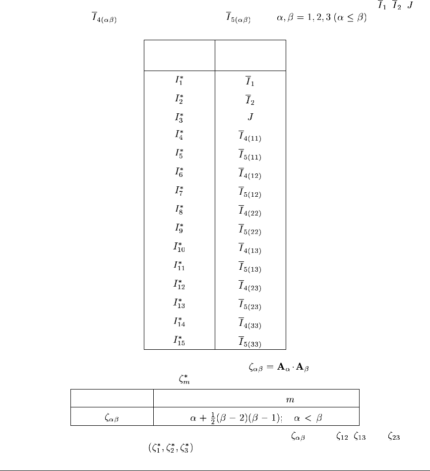
UANISOHYPER_INV
For example, in the case of three families of fibers there a re a total of 15 invariants: , , ,six
invariants of type
, and six invariants of type ,with . The following
correspondence exists between each of these invariants and their enumerated counterpart:
Enumerated
invariant
Invariant
A similar scheme is used for the array ZETA of terms . Each term can be represented
uniquely by an enumerated counterpart
, as shown below:
Dot product Enumeration,
As an example, for the case of three families of fibers there are three terms: , ,and .These
arestoredintheZETA array as
.
Storage of arrays of derivatives of the energy function
The components of the array UI1 of first derivatives of the strain energy potential with respect to the
1.1.20–2
Abaqus ID:
Printed on:

UANISOHYPER_INV
scalar invariants, , are stored using the enumeration schem e discussed above for the scalar
invariants.
The elements of the array UI2 of second derivatives of the strain energy function,
,
are laid out in memory using triangular storage: if
denotes the component in this array corres ponding
to the term
,then . For exam ple, the term is
stored in component
in the UI2 array.
Special considerations for various element types
There are several special considerations that need to be noted.
Shells that calculate transverse shear energy
When UANISOHYPER_INV is used to define the materia l response of shell elements that calculate
transverse shear energy, Abaqus/Standard cannot calculate a default value for the transverse shear
stiffness of the element. Hence, you must define the element’s transverse shear stiffness. See “Shell
section behavior,” Section 26.6.4 of the Abaqus Analysis User’s Manual, for guidelines on choosing
this stiffness.
Elements with hourglassing modes
When UANISOHYPER_INV is used to define the material response of elements with hourglassing
modes, you must define the hourglass stiffness for hourglass control based on the total stiffness
approach. The hourglass stiffness is not required for enhance d hourglass control, but you can define a
scaling factor for the stiffness associated w ith the drill degree of freedom (rotation about the surface
normal). See “Section controls,” Section 24.1.4 of the Abaqus Analysis User’s Manual.
User subroutine interface
SUBROUTINE UANISOHYPER_INV (AINV, UA, ZETA, NFIBERS, NINV,
1 UI1, UI2, UI3, TEMP, NOEL, CMNAME, INCMPFLAG, IHYBFLAG,
2 NUMSTATEV, STATEV, NUMFIELDV, FIELDV, FIELDVINC,
3 NUMPROPS, PROPS)
C
INCLUDE 'ABA_PARAM.INC'
C
CHARACTER*80 CMNAME
DIMENSION AINV(NINV), UA(2),
2 ZETA(NFIBERS*(NFIBERS-1)/2)), UI1(NINV),
3 UI2(NINV*(NINV+1)/2), UI3(NINV*(NINV+1)/2),
4 STATEV(NUMSTATEV), FIELDV(NUMFIELDV),
5 FIELDVINC(NUMFIELDV), PROPS(NUMPROPS)
user coding to define UA,UI1,UI2,UI3,STATEV
RETURN
END
1.1.20–3
Abaqus ID:
Printed on:

UANISOHYPER_INV
Variables to be defined
UA(1)
U, strain energy density function. For a compressible material at least one derivative involving J should
be nonzero. For an incompressible mater ial all derivatives involving J are ignored.
UA(2)
, the deviatoric part of the strain energy density of the primary material response. This quantity
is needed only if the current material definition also includes Mullins effect (see “Mullins effect in
rubberlike m aterials,” Section 19.6.1 of the Abaqus Analysis User’s Manual).
UI1(NINV)
Array of derivatives of strain energy potential with respect to the scalar invariants,
, ordered
using the enum eration scheme discussed above.
UI2(NINV*(NINV+1)/2)
Array of second derivatives of strain energy potential with respect to the scalar invariants (using
triangular storage),
.
UI3(NINV*(NINV+1)/2)
Array of derivatives with respect to J of the s econd derivatives of the strain energy potential (using
triangular storage),
. This quantity is needed only for compressible materials with a
hybrid form ulation (when INCMPFLAG =0andIHYBFLAG =1).
STATEV
Array containing the user-defined solution-dependent state variables at this point. These are supplied a s
values at the start of the increment or as values updated by other user subroutines (see “User subroutines:
overview,” Section 15.1.1 of the Abaqus Analysis User’s Manual) and must be returned as values at
the end of the increment.
Variables passed in for information
NFIBERS
Number of families of fibers defined for this material.
NINV
Number of scalar invariants.
TEMP
Current temperature at this point.
NOEL
Element number.
1.1.20–4
Abaqus ID:
Printed on:

UANISOHYPER_INV
CMNAME
User-specified material name, left justified.
INCMPFLAG
Incompressibility flag defined to be 1 if the material is specified as incompressible or 0 if the m aterial
is specified as compressible.
IHYBFLAG
Hybrid formulation flag defined to be 1 for hybrid elements; 0 otherwise.
NUMSTATEV
User-defined number of solution-dependent state variables associated with this material (see
“Allocating space” in “U ser subroutines: overview,” Section 15.1.1 of the A baqus Analysis User’s
Manual).
NUMFIELDV
Number of field variables.
FIELDV
Array of interpolated values of predefined field variables at this material point at the end of the
increment based on the values read in at the nodes (initial values at the beginning of the analysis and
current values during the analysis).
FIELDVINC
Array of increments of predefined field variables at this material point for this increment, including any
values updated by user subroutine USDFLD.
NUMPROPS
Number of material properties entered for this user-defined hyperelastic m aterial.
PROPS
Array of material properties entered for this user-defined hyperelastic m aterial.
AINV(NINV)
Array of scalar invariants,
, at each material point at the end of the increment. The invariants are
ordered using the enumeration scheme discus sed above.
ZETA(NFIBERS*(NFIBERS-1)/2))
Array of dot product between the directions of different fam ilies of fiber in the reference configuration,
. The array contains the enumerated values using the scheme discussed above.
1.1.20–5
Abaqus ID:
Printed on:

UANISOHYPER_INV
Example: Anisotropic hyperelastic model of Kaliske and Schmidt
As an example of the coding of user subroutine UANISOHYPER_INV, consider the model proposed by
Kaliske and Schmidt (2005) for nonlinear anisotropic elasticity with two families of fi bers. The strain
energy function is given by a polynom ial series expansion in the form
The code in user subroutine UANISOHYPER_INV must return the derivatives of the strain energy
function with respect to the scalar invariants, w hich are readily computed from the above expression. In
this example auxiliary functions are used to facilitate enumeration of pseudo -invariants of type
and , as well as for indexing into the array of second derivatives using symmetric storage. The
user subroutine would be coded as follows:
subroutine uanisohyper_inv (aInv, ua, zeta, nFibers, nInv,
* ui1, ui2, ui3, temp, noel,
* cmname, incmpFlag, ihybFlag,
* numStatev, statev,
* numFieldv, fieldv, fieldvInc,
* numProps, props)
c
include 'aba_param.inc'
c
character *80 cmname
dimension aInv(nInv), ua(2), zeta(nFibers*(nFibers-1)/2)
dimension ui1(nInv), ui2(nInv*(nInv+1)/2)
dimension ui3(nInv*(nInv+1)/2), statev(numStatev)
dimension fieldv(numFieldv), fieldvInc(numFieldv)
dimension props(numProps)
C
parameter ( zero = 0.d0,
* one = 1.d0,
* two = 2.d0,
* three = 3.d0,
* four = 4.d0,
* five = 5.d0,
* six = 6.d0 )
C
1.1.20–6
Abaqus ID:
Printed on:
UANISOHYPER_INV
C Kaliske-Schmidtt energy function (3D)
C
C Read material properties
d=props(1)
dInv = one / d
a1=props(2)
a2=props(3)
a3=props(4)
b1=props(5)
b2=props(6)
b3=props(7)
c2=props(8)
c3=props(9)
c4=props(10)
c5=props(11)
c6=props(12)
d2=props(13)
d3=props(14)
d4=props(15)
d5=props(16)
d6=props(17)
e2=props(18)
e3=props(19)
e4=props(20)
e5=props(21)
e6=props(22)
f2=props(23)
f3=props(24)
f4=props(25)
f5=props(26)
f6=props(27)
g2=props(28)
g3=props(29)
g4=props(30)
g5=props(31)
g6=props(32)
C
C Compute Udev and 1st and 2nd derivatives w.r.t invariants
C-I1
bi1 = aInv(1)
term = bi1-three
ua(2) = a1*term + a2*term**2 + a3*term**3
1.1.20–7
Abaqus ID:
Printed on:
UANISOHYPER_INV
ui1(1) = a1 + two*a2*term + three*a3*term**2
ui2(indx(1,1)) = two*a2 + three*two*a3*term
C - I2 bi2 = aInv(2)
term = bi2-three
ua(2) = ua(2) + b1*term + b2*term**2 + b3*term**3
ui1(2) = b1 + two*b2*term + three*b3*term**2
ui2(indx(2,2)) = two*b2 + three*two*b3*term
C - I3 (=J)
bi3 = aInv(3)
term = bi3-one
ui1(3) = two*dInv*term
ui2(indx(3,3)) = two*dInv
C - I4(11)
nI411 = indxInv4(1,1)
bi411 = aInv(nI411)
term = bi411-one
ua(2) = ua(2)
* + c2*term**2 + c3*term**3 + c4*term**4
* + c5*term**5 + c6*term**6
ui1(nI411) =
* two*c2*term
* + three*c3*term**2
* + four*c4*term**3
* + five*c5*term**4
* + six*c6*term**5
ui2(indx(nI411,nI411)) =
* two*c2
* + three*two*c3*term
* + four*three*c4*term**2
* + five*four*c5*term**3
* + six*five*c6*term**4
C - I5(11)
nI511 = indxInv5(1,1)
bi511 = aInv(nI511)
term = bi511-one
ua(2) = ua(2)
* + d2*term**2 + d3*term**3 + d4*term**4
* + d5*term**5 + d6*term**6
ui1(nI511) =
* two*d2*term
* + three*d3*term**2
* + four*d4*term**3
1.1.20–8
Abaqus ID:
Printed on:
UANISOHYPER_INV
* + five*d5*term**4
* + six*d6*term**5
ui2(indx(nI511,nI511)) =
* two*d2
* + three*two*d3*term
* + four*three*d4*term**2
* + five*four*d5*term**3
* + six*five*d6*term**4
C - I4(22)
nI422 = indxInv4(2,2)
bi422 = aInv(nI422)
term = bi422-one
ua(2) = ua(2)
* + e2*term**2 + e3*term**3 + e4*term**4
* + e5*term**5 + e6*term**6
ui1(nI422) =
* two*e2*term
* + three*e3*term**2
* + four*e4*term**3
* + five*e5*term**4
* + six*e6*term**5
ui2(indx(nI422,nI422)) =
* two*e2
* + three*two*e3*term
* + four*three*e4*term**2
* + five*four*e5*term**3
* + six*five*e6*term**4
C - I5(22)
nI522 = indxInv5(2,2)
bi522 = aInv(nI522)
term = bi522-one
ua(2) = ua(2)
* + f2*term**2 + f3*term**3 + f4*term**4
* + f5*term**5 + f6*term**6
ui1(nI522) =
* two*f2*term
* + three*f3*term**2
* + four*f4*term**3
* + five*f5*term**4
* + six*f6*term**5
ui2(indx(nI522,nI522)) =
* two*f2
1.1.20–9
Abaqus ID:
Printed on:
UANISOHYPER_INV
* + three*two*f3*term
* + four*three*f4*term**2
* + five*four*f5*term**3
* + six*five*f6*term**4
C - I4(12)
nI412 = indxInv4(1,2)
bi412 = aInv(nI412)
term = zeta(1)*(bi412-zeta(1))
ua(2) = ua(2)
* + g2*term**2 + g3*term**3
* + g4*term**4 + g5*term**5
* + g6*term**6
ui1(nI412) = zeta(1) * (
* two*g2*term
* + three*g3*term**2
* + four*g4*term**3
* + five*g5*term**4
* + six*g6*term**5 )
ui2(indx(nI412,nI412)) = zeta(1)**2 * (
* two*g2
* + three*two*g3*term
* + four*three*g4*term**2
* + five*four*g5*term**3
* + six*five*g6*term**4 )
C
c Add volumetric energy
c
term = aInv(3) - one
ua(1) = ua(2) + dInv*term*term
C
return
end
*
* Maps index from Square to Triangular storage of symmetric
matrix integer function indx( i, j )
*
include 'aba_param.inc'
*
ii = min(i,j)
jj = max(i,j)
*
indx = ii + jj*(jj-1)/2
1.1.20–10
Abaqus ID:
Printed on:

UANISOHYPER_INV
*
return
end
*
*
* Generate enumeration of Anisotropic Pseudo Invariants of
type 4 integer function indxInv4( i, j )
*
include 'aba_param.inc'
*
ii = min(i,j)
jj = max(i,j)
*
indxInv4=4+jj*(jj-1) + 2*(ii-1)
*
return
end
*
*
* Generate enumeration of Anisotropic Pseudo Invariants of
type 5 integer function indxInv5( i, j )
*
include 'aba_param.inc'
*
ii = min(i,j)
jj = max(i,j)
*
indxInv5=5+jj*(jj-1) + 2*(ii-1)
*
return
end
Additional reference
•
Kaliske, M., and J. Schmidt, “Formulation of Finite Nonlinear Anisotropic Elasticity,” CADFEM
GmbH Infoplaner 2/2005, vol. 2, pp. 22–23, 2005.
1.1.20–11
Abaqus ID:
Printed on:

UANISOHYPER_STRAIN
1.1.21 UANISOHYPER_STRAIN: User subroutine to define anisotropic hyperelastic
material behavior based on Green strain.
Product:
Abaqus/Standard
References
•
“Anisotropic hyperelastic behavior,” Section 19.5.3 of the Abaqus Analysis User’s Manual
• *
ANISOTROPIC HYPERELASTIC
•
“UANISOHYPER_INV and VUANISOHYPER_INV,” Section 4.1.13 of the Abaqus Verification
Manual
Overview
User subroutine UANISOHYPER_STRAIN:
•
can be used to define the stra in energy potential of anisotropic hype relastic materials as a f unction
of the components of the Green str ain tensor;
•
is called at all material calculation points of elements for which the m aterial definition contains
user-defined anisotropic hyperelastic behavior w ith a Green strain-based formulation (“Anisotropic
hyperelastic behavior,” Section 19 .5.3 of the Abaqus Analysis User’s Manual);
•
can include m aterial behavior dependent on field variables or state variables; and
•
requires that the values of the derivatives of the strain energy density function of the anisotropic
hyperelastic material be defined with respect to the components of the modified Green strain tensor.
Storage of strain components
In the array of modified Green strain, EBAR, direct components are stored first, followed by shear
components. There are NDI direct and NSHR tensor shear components. The order of the components is
defined in “Conventions,” Section 1.2.2 of the Abaqus Analysis User’s M anual. Since the number of
active stress and strain components varies between element types, the routine m ust be coded to provide
for all element types with which it will be used.
Storage of arrays of derivatives of the energy function
The array of first derivatives of the strain energy function, DU1, contains NTENS+1 components, with
NTENS=NDI+NSHR. The first NTENS components correspond to the derivatives with respect to each
component of the modified Green strain,
. The last component contains the de rivative with
respect to the volume ratio,
.
The array of second derivatives of the strain energy function, DU2, contains
(NTENS+1)*(NTENS+2)/2 components. These components are ordered using the following
triangular storage scheme:
1.1.21–1
Abaqus ID:
Printed on:

UANISOHYPER_STRAIN
Component 2-D Case 3-D Case
1
2
3
4
5
6
7
8
9
10
11
12
13
14
15
16
17
18
19
20
21
22
23
24
25
26
1.1.21–2
Abaqus ID:
Printed on:

UANISOHYPER_STRAIN
Component 2-D Case 3-D Case
27
28
Finally, the array of third derivatives of the strain energy function, DU3, also contains
(NTENS+1)*(NTENS+2)/2 components, each representing the derivative with respect to
of the
corresponding component of DU2. It follows the same triangular storage scheme as DU2.
Special considerations for various element types
There are several special considerations that need to be noted.
Shells that calculate transverse shear energy
When UANISOHYPER_STRAIN is used to define the material response of shell elements that calculate
transverse shear energy, Abaqus/Standard cannot calculate a default value for the transverse shear
stiffness of the element. Hence, you must define the element’s transverse shear stiffness. See “Shell
section behavior,” Section 26.6.4 of the Abaqus Analysis User’s Manual, for guidelines on choosing
this stiffness.
Elements with hourglassing modes
When UANISOHYPER_STRAIN is used to define the material response of elements with hourglassing
modes, you must define the hourglas s stiffness for hourglass control based on the total stiffness a pproach.
The hourglass stiffness is not required for enhanced hourglass control, but you can define a scaling factor
for the stiffness associated with the drill degree of freedom (rotation about the surface normal). See
“Section controls,” Section 24.1.4 of the Abaqus Analysis User’s Manual.
User subroutine interface
SUBROUTINE UANISOHYPER_STRAIN (EBAR, AJ, UA, DU1, DU2, DU3,
1 TEMP, NOEL, CMNAME, INCMPFLAG, IHYBFLAG, NDI, NSHR, NTENS,
2 NUMSTATEV, STATEV, NUMFIELDV, FIELDV, FIELDVINC,
3 NUMPROPS, PROPS)
C
INCLUDE 'ABA_PARAM.INC'
C
CHARACTER*80 CMNAME
C
DIMENSION EBAR(NTENS), UA(2), DU1(NTENS+1),
2 DU2((NTENS+1)*(NTENS+2)/2),
3 DU3((NTENS+1)*(NTENS+2)/2),
1.1.21–3
Abaqus ID:
Printed on:

UANISOHYPER_STRAIN
4 STATEV(NUMSTATEV), FIELDV(NUMFIELDV),
5 FIELDVINC(NUMFIELDV), PROPS(NUMPROPS)
user coding to define UA,DU1,DU2,DU3,STATEV
RETURN
END
Variables to be defined
UA(1)
U, strain energy density function. For a compressible material at least one derivative involving J should
be nonzero. For an incompressible mater ial all derivatives involving J are ignored.
UA(2)
, the deviatoric part of the strain energy density of the primary material response. This quantity
is needed only if the current material definition also includes Mullins effect (see “Mullins effect in
rubberlike m aterials,” Section 19.6.1 of the Abaqus Analysis User’s Manual).
DU1(NTENS+1)
Derivatives of strain energy potential with respect to the components of the modified Green strain
tensor,
, and with respect to the volu me ratio, .
DU2((NTENS+1)*(NTENS+2)/2)
Second derivatives of strain energy potential with respect to the co mponents of the modified Green
strain tensor and the volume ratio (using triangular storage, as mentioned earlier).
DU3((NTENS+1)*(NTENS+2)/2)
Derivatives with respect to J of the second de rivatives of the strain ene rgy potential (using triangular
storage, as mentioned earlier). This quantity is needed only for compressible materials w ith a hybrid
formulation (when INCMPFLAG =0andIHYBFLAG =1).
STATEV
Array containing the user-defined solution-dependent state variables at this point. These are supplied a s
values at the start of the increment or as values updated by other user subroutines (see “User subroutines:
overview,” Section 15.1.1 of the Abaqus Analysis User’s Manual) and must be returned as values at
the end of the increment.
Variables passed in for information
TEMP
Current temperature at this point.
1.1.21–4
Abaqus ID:
Printed on:
UANISOHYPER_STRAIN
NOEL
Element number.
CMNAME
User-specified material name, left justified.
NDI
Number of direct stress components at this point.
NSHR
Number of shear components at this point.
NTENS
Size of the stress or strain component array (NDI + NSHR).
INCMPFLAG
Incompressibility flag defined to be 1 if the material is specified as incompressible or 0 if the m aterial
is specified as compressible.
IHYBFLAG
Hybrid formulation flag defined to be 1 for hybrid elements; 0 otherwise.
NUMSTATEV
User-defined number of solution-dependent state variables associated with this material (see
“Allocating space” in “U ser subroutines: overview,” Section 15.1.1 of the A baqus Analysis User’s
Manual).
NUMFIELDV
Number of field variables.
FIELDV
Array of interpolated values of predefined field variables at this material point at the end of the
increment based on the values read in at the nodes (initial values at the beginning of the analysis and
current values during the analysis).
FIELDVINC
Array of increments of predefined field variables at this material point for this increment, including any
values updated by user subroutine USDFLD.
NUMPROPS
Number of material properties entered for this user-defined hyperelastic m aterial.
PROPS
Array of material properties entered for this user-defined hyperelastic m aterial.
1.1.21–5
Abaqus ID:
Printed on:

UANISOHYPER_STRAIN
EBAR(NTENS)
Modified Green strain tensor,
, at the material point at the end of the increm ent.
AJ
J, determinant of deformation gradient (volume ratio) at the end of the increment.
Example: Orthotropic Saint-Venant Kirchhoff model
As a simple example of the coding of user subroutine UANISOHYPER_STRAIN, consider the
generalization to anisotropic hypere lasticity of the Sa int-Venant Kirchhoff model. The strain energy
function of the Saint-Venant Kirchhoff model can be expressed as a quadratic function of the Green
strain tensor,
,as
where is the fourth-order elasticity tensor. The derivatives of the strain energy function with respect
to the G reen strain are given as
However, user subroutine UANISOHYPER_STRAIN must return the derivatives of the strain energy
function with respect to the modified Green strain tensor,
, and the volume rati o, J, which can be
accomplished easily using the following relationship between
, ,and :
where is the second-order identity tensor. Thus, using the chain rule we find
1.1.21–6
Abaqus ID:
Printed on:

UANISOHYPER_STRAIN
where
and
In this example an auxiliary function is used to facilitate indexing into a fourth-order symmetric
tensor. The user subroutine would be code d as follows:
subroutine uanisohyper_strain (
* ebar, aj, ua, du1, du2, du3, temp, noel, cmname,
* incmpFlag, ihybFlag, ndi, nshr, ntens,
* numStatev, statev, numFieldv, fieldv, fieldvInc,
* numProps, props)
c
include 'aba_param.inc'
c
dimension ebar(ntens), ua(2), du1(ntens+1)
dimension du2((ntens+1)*(ntens+2)/2)
dimension du3((ntens+1)*(ntens+2)/2)
dimension statev(numStatev), fieldv(numFieldv)
dimension fieldvInc(numFieldv), props(numProps)
c
character*80 cmname
c
parameter ( half = 0.5d0,
$ one = 1.d0,
$ two = 2.d0,
$ third = 1.d0/3.d0,
$ twothds = 2.d0/3.d0,
$ four = 4.d0 )
*
* Orthotropic Saint-Venant Kirchhoff strain energy function (3D)
*
D1111=props(1)
D1122=props(2)
D2222=props(3)
1.1.21–7
Abaqus ID:
Printed on:
UANISOHYPER_STRAIN
D1133=props(4)
D2233=props(5)
D3333=props(6)
D1212=props(7)
D1313=props(8)
D2323=props(9)
*
d2UdE11dE11 = D1111
d2UdE11dE22 = D1122
d2UdE11dE33 = D1133
*
d2UdE22dE11 = d2UdE11dE22
d2UdE22dE22 = D2222
d2UdE22dE33 = D2233
*
d2UdE33dE11 = d2UdE11dE33
d2UdE33dE22 = d2UdE22dE33
d2UdE33dE33 = D3333
*
d2UdE12dE12 = D1212
*
d2UdE13dE13 = D1313
*
d2UdE23dE23 = D2323
*
xpow = exp ( log(aj) * twothds )
detuInv = one / aj
*
E11 = xpow * ebar(1) + half * ( xpow - one )
E22 = xpow * ebar(2) + half * ( xpow - one )
E33 = xpow * ebar(3) + half * ( xpow - one )
E12 = xpow * ebar(4)
E13 = xpow * ebar(5)
E23 = xpow * ebar(6)
*
term1 = twothds * xpow * detuInv
dE11Dj = term1 * ( E11 + half )
dE22Dj = term1 * ( E22 + half )
dE33Dj = term1 * ( E33 + half )
dE12Dj = term1 * E12
dE13Dj = term1 * E13
dE23Dj = term1 * E23
1.1.21–8
Abaqus ID:
Printed on:
UANISOHYPER_STRAIN
term2 = - third * detuInv
d2E11DjDj = term2 * dE11Dj
d2E22DjDj = term2 * dE22Dj
d2E33DjDj = term2 * dE33Dj
d2E12DjDj = term2 * dE12Dj
d2E13DjDj = term2 * dE13Dj
d2E23DjDj = term2 * dE23Dj
*
dUdE11 = d2UdE11dE11 * E11
* + d2UdE11dE22 * E22
* + d2UdE11dE33 * E33
dUdE22 = d2UdE22dE11 * E11
* + d2UdE22dE22 * E22
* + d2UdE22dE33 * E33
dUdE33 = d2UdE33dE11 * E11
* + d2UdE33dE22 * E22
* + d2UdE33dE33 * E33
dUdE12 = two * d2UdE12dE12 * E12
dUdE13 = two * d2UdE13dE13 * E13
dUdE23 = two * d2UdE23dE23 * E23
*
U = half * ( E11*dUdE11 + E22*dUdE22 + E33*dUdE33 )
* + E12*dUdE12 + E13*dUdE13 + E23*dUdE23
*
ua(2) = U
ua(1) = ua(2)
*
du1(1) = xpow * dUdE11
du1(2) = xpow * dUdE22
du1(3) = xpow * dUdE33
du1(4) = xpow * dUdE12
du1(5) = xpow * dUdE13
du1(6) = xpow * dUdE23
du1(7) = dUdE11*dE11Dj + dUdE22*dE22Dj + dUdE33*dE33Dj
* + two * ( dUdE12*dE12Dj
* +dUdE13*dE13Dj
* +dUdE23*dE23Dj )
*
xpow2 = xpow * xpow
*
du2(indx(1,1)) = xpow2 * d2UdE11dE11
du2(indx(1,2)) = xpow2 * d2UdE11dE22
1.1.21–9
Abaqus ID:
Printed on:
UANISOHYPER_STRAIN
du2(indx(2,2)) = xpow2 * d2UdE22dE22
du2(indx(1,3)) = xpow2 * d2UdE11dE33
du2(indx(2,3)) = xpow2 * d2UdE22dE33
du2(indx(3,3)) = xpow2 * d2UdE33dE33
du2(indx(1,4)) = zero
du2(indx(2,4)) = zero
du2(indx(3,4)) = zero
du2(indx(4,4)) = xpow2 * d2UdE12dE12
du2(indx(1,5)) = zero
du2(indx(2,5)) = zero
du2(indx(3,5)) = zero
du2(indx(4,5)) = zero
du2(indx(5,5)) = xpow2 * d2UdE13dE13
du2(indx(1,6)) = zero
du2(indx(2,6)) = zero
du2(indx(3,6)) = zero
du2(indx(4,6)) = zero
du2(indx(5,6)) = zero
du2(indx(6,6)) = xpow2 * d2UdE23dE23
*
du2(indx(1,7)) = term1 * dUdE11 + xpow * (
* d2UdE11dE11 * dE11Dj
* + d2UdE11dE22 * dE22Dj
* + d2UdE11dE33 * dE33Dj )
du2(indx(2,7)) = term1 * dUdE22 + xpow * (
* d2UdE22dE11 * dE11Dj
* + d2UdE22dE22 * dE22Dj
* + d2UdE22dE33 * dE33Dj )
du2(indx(3,7)) = term1 * dUdE33 + xpow * (
* + d2UdE33dE11 * dE11Dj
* + d2UdE33dE22 * dE22Dj
* + d2UdE33dE33 * dE33Dj )
du2(indx(4,7)) = term1 * dUdE12
* + xpow * two * d2UdE12dE12 * dE12Dj
du2(indx(5,7)) = term1 * dUdE13
* + xpow * two * d2UdE13dE13 * dE23Dj
du2(indx(6,7)) = term1 * dUdE23
* + xpow * two * d2UdE23dE23 * dE13Dj
du2(indx(7,7))= dUdE11*d2E11DjDj
* +dUdE22*d2E22DjDj
* +dUdE22*d2E22DjDj
* + two*( dUdE12*d2E12DjDj
1.1.21–10
Abaqus ID:
Printed on:
UANISOHYPER_STRAIN
* +dUdE13*d2E13DjDj
* +dUdE23*d2E23DjDj)
* + d2UdE11dE11 * dE11Dj * dE11Dj
* + d2UdE22dE22 * dE22Dj * dE22Dj
* + d2UdE33dE33 * dE33Dj * dE33Dj
* + two * ( d2UdE11dE22 * dE11Dj * dE22Dj
* +d2UdE11dE33 * dE11Dj * dE33Dj
* +d2UdE22dE33 * dE22Dj * dE33Dj )
* + four * ( d2UdE12dE12 * dE12Dj * dE12Dj
* d2UdE13dE13 * dE13Dj * dE13Dj
* d2UdE23dE23 * dE23Dj * dE23Dj )
*
return
end
*
* Maps index from Square to Triangular storage
* of symmetric matrix
*
integer function indx( i, j )
*
include 'aba_param.inc'
*
ii = min(i,j)
jj = max(i,j)
*
indx = ii + jj*(jj-1)/2
*
return
end
1.1.21–11
Abaqus ID:
Printed on:

UCORR
1.1.22 UCORR: User subroutine to define cross-correlation properties for random
response loading.
Product:
Abaqus/Standard
References
•
“Random response analysis,” Section 6.3.11 of the Abaqus Analysis User’s Manual
• *
CORRELATION
•
“Random response to jet noise e xcitation,” Section 1.4.10 of th e Abaqus Benchmarks Manua l
Overview
User subroutine UCORR:
•
can be used to define the coefficients for the cross-correlation matrix in a random response analysis;
•
will be called once for the combination of any two degrees of freedom with nonzero prescribed
loads for each load case specified as a concentrated or distributed load or once for the combination
of any two excitation directions specified as a base motion;
•
allows correlation coefficients to be defined as a function of nodal coordinates; and
•
ignores any data specified outside the user subroutine for the associated cross-correlation matrix.
Cross-correlation for base motion excitation
The spatial correlation matrix for base motion excitation is defined by the coefficients in user
subroutine UCORR,where
are excitation directions and J corresponds to the Jth frequency function
referenced under load case I.
Cross-correlation for point loads and distributed loads
The spatial correlation matrix of the load is defined as follows. Let be the load applied to degree of
freedom i at node N in load case I, through the use of a concentrated or distributed load. Let J correspond
to the Jth frequency function referenced under load case I. The spatial correlation matri x used in the
random response analysis for this load case is then
where are the coefficients defined in user subroutine UCORR. Typically the load magnitude
is given as 1.0; therefore, the load definition is simply selecting the nonzero terms that will appear in
.
1.1.22–1
Abaqus ID:
Printed on:

UCORR
User subroutine interface
SUBROUTINE UCORR(PSD,CORRR,CORRI,KSTEP,LCASE,JNODE1,JDOF1,
1 JNODE2,JDOF2,COOR1,COOR2)
C
INCLUDE 'ABA_PARAM.INC'
C
DIMENSION COOR1(3),COOR2(3)
CHARACTER*80 PSD
user coding to define CORRR and CORRI
RETURN
END
Variables to be defined
CORRR
Real part of the cross-correlation scaling factor.
CORRI
Imaginary part of the cross-correlation scaling factor.
Variables passed in for information
PSD
User-specified name for the frequency function that references this correlation, left justified.
KSTEP
Step number.
LCASE
Load case number, I.
JNODE1
First node involved, N (not used for base motion excitation).
JDOF1
Degree of freedom i at the first node (for concentrated or distributed load excitation) or global excita tion
direction i (for base motion excitation).
JNODE2
Second node involved, M (not used for base motion exc itation).
1.1.22–2
Abaqus ID:
Printed on:
UCORR
JDOF2
Degree of freedom j at the second node (for concentrated or distributed load excitation) or global
excitation direction j (for base motion excitation).
COOR1
An array containing the coordinates of the first node (not used for base motion excitation).
COOR2
An array containing the coordinates of the second node (not used for base motion exc itation).
1.1.22–3
Abaqus ID:
Printed on:

UEL
1.1.23 UEL: User subroutine to define an element.
Product:
Abaqus/Standard
WARNING: This feature is intended f or advanced users only. Its use in all but the
simplest test examples will require considerable coding by the user/developer.
“User-defined elements,” Section 29.16.1 of the Abaqus Analysis User’s Manual,
should be read before proceeding.
References
•
“User-defined elements,” Section 29.16.1 of the Abaqus A nalysis User’s Manual
• *
UEL PROPERTY
• *
USER ELEMENT
Overview
User subroutine UEL:
•
will be called for each element that is of a general user-defined elem ent type (i.e., not defined by
a linear stiffness or mass matrix read either directly or from results file data) each tim e element
calculations are required; and
•
(or subroutines called by user s ubroutine UEL) m ust perform all of the calculations for the element,
appropriate to the current activity in the analysis.
Wave kinematic data
For Abaqus/Aqua applica tions four utility routines—GETWAVE, GETWAVEVEL, GETWINDVEL,and
GETCURRVEL—are provided to access the fluid kinematic data. These routines are used from within
user subroutine UEL and are discussed in detail in “Obtaining wave kinem atic data in an Abaqus/Aqua
analysis,” Section 2.1.13.
User subroutine interface
SUBROUTINE UEL(RHS,AMATRX,SVARS,ENERGY,NDOFEL,NRHS,NSVARS,
1 PROPS,NPROPS,COORDS,MCRD,NNODE,U,DU,V,A,JTYPE,TIME,DTIME,
2 KSTEP,KINC,JELEM,PARAMS,NDLOAD,JDLTYP,ADLMAG,PREDEF,NPREDF,
3 LFLAGS,MLVARX,DDLMAG,MDLOAD,PNEWDT,JPROPS,NJPROP,PERIOD)
C
INCLUDE 'ABA_PARAM.INC'
C
DIMENSION RHS(MLVARX,*),AMATRX(NDOFEL,NDOFEL),PROPS(*),
1 SVARS(*),ENERGY(8),COORDS(MCRD,NNODE),U(NDOFEL),
1.1.23–1
Abaqus ID:
Printed on:

UEL
2 DU(MLVARX,*),V(NDOFEL),A(NDOFEL),TIME(2),PARAMS(*),
3 JDLTYP(MDLOAD,*),ADLMAG(MDLOAD,*),DDLMAG(MDLOAD,*),
4 PREDEF(2,NPREDF,NNODE),LFLAGS(*),JPROPS(*)
user coding to define RHS, AMATRX, SVARS, ENERGY, and PNEWDT
RETURN
END
Variables to be defined
These arrays depend on the value of the LFLAGS array.
RHS
An array containing the contribu tions of this element to the right-hand- side vectors of the overa ll system
of equations. For most nonlinear analysis procedures, NRHS=1 and RHS should contain the residual
vector. The exception is the modified Riks static procedure (“Static stress analysis,” Section 6.2.2 of the
Abaqus Analysis User’s Manual), for which NRHS=2 and the first column in RHS should contain the
residual vector and the second column should contain the increments of external load on the elem ent.
RHS(K1,K2) is the entry for the K1th degree of freedom of the element in the K2th right-hand-side
vector.
AMATRX
An array containing the contribution of this element to the Jacobian (stiffness) o r other matrix of the
overall system of equations. The particular matrix required at any time depends on th e entries in the
LFLAGS array (see below).
All nonzero entries in AMATRX should be defined, even if the matrix is symme tric. If you do
not specify that the matrix is unsymmetric when you define the user element, Abaqus/Standard will
use the symmetri c ma trix defined by
,where is the m atrix defined as AMATRX
in this subroutine. If you specify that the matrix is unsymmetric when you define the user elem ent,
Abaqus/Standard will use AMATRX directly.
SVARS
An array containing the values of the solution-dependent state variables associated with this element.
The number of such variables is NSVARS (see below). You define the meaning of these variables.
For general nonlinear steps this array is passed into UEL containing the values of these var iables at
the start of the current increment. They should be updated to be the values at the end of the increment,
unless the procedure during w hich UEL is being called does not require such an update. This depends
on the entries in the LFLAGS array (see below). For linear pertur bation steps this array is passed into
UEL containing the values of these variables in the base state. They should be returned containing
perturbation values if you wish to output such quantities.
1.1.23–2
Abaqus ID:
Printed on:

UEL
When KINC is equal to zero, the call to UEL is made for zero increm ent output (see “Output,”
Section 4.1.1 of the Abaqus Analysis User’s Manual). In this case the values returned will be used only
for output purposes and are not updated permanently.
ENERGY
For general nonlinear steps array ENERGY contains the values of the energy quantities associated with
the element. The values in this array w hen UEL is called are the element energy quantities at the sta rt
of the current increm ent. They should be updated to the values at the end of the current increment.
For linear perturbation steps the array is passed into UEL containing the energy in the base state. They
should be returned containing perturbation values if you wish to output such quantities. The entries in
the array are as follows:
ENERGY(1) Kinetic ene rgy.
ENERGY(2) Elastic strain energy.
ENERGY(3) Creep dissipation.
ENERGY(4) Plastic dissi pation.
ENERGY(5) Viscous dissipation.
ENERGY(6) “Artificial strain energy” associated with such effects as artificial
stiffness introduced to control hourglassing or other singular modes
in the element.
ENERGY(7) Electrostatic energy.
ENERGY(8) Incremental work done by loads applied within the user element.
When KINC is equal to zero, the call to UEL is made for zero increm ent output (see “Output,”
Section 4.1.1 of the Abaqus Analysis User’s Manual). In this case the energy values returned will be
used only for output purposes and are not upda ted permanently.
Variable that can be updated
PNEWDT
Ratio of s uggested new time inc rement to the tim e increment currently being used (DTIME,see
below). This variable allows you to provide input to the automatic t ime incrementation algorithms in
Abaqus/Standard (if automatic time incrementation is chosen). It is useful only during equilibrium
iterations with the normal time incrementation, as indicated by LFLAGS(3)=1. During a severe
discontinuity iteration (such as contact changes), PNEWDT is ignored unless CONV ERT SDI=YES is
specified for this step. The usage of PNEWDT is discussed below.
PNEWDT is set to a large value before each call to UEL.
If PNEWDT is redefined to be less than 1.0, Abaqus/Standard must abandon the time increment
and attem pt it again with a smaller time increment. The suggested new time increment provided to the
automatic time integration algorithms is PNEWDT × DTIME, wher e the PNEWDT used is the minimum
value for all calls to user subroutines that allow redefinition of PNEWDT for this iteration.
1.1.23–3
Abaqus ID:
Printed on:

UEL
If PNEWDT is given a v alue that is greater than 1.0 for all calls to user subroutines for this iteration
and the increment converges in this iteration, A baqus/Standard m ay increase the time increment. The
suggested new time increment provided to the automatic time integration algorithms is PNEWDT ×
DTIME, where the PNEWDT used is the minimum value for all calls to user subroutines for this iteration.
If automatic time incrementation is not selected in the anal ysis proc edure, values of PNEWDT that
are greater than 1.0 will be ignored and values of PNEWDT that are less than 1.0 will cause the job to
terminate.
Variables passed in for information
Arrays:
PROPS
A floating point array containing the NPROPS real property values defined for use with this element.
NPROPS is the user-specified number of real property values. See “D efining the elem ent properties”
in “User-defined elements,” Section 29.16.1 of the Abaqus Analysis User’s Manual.
JPROPS
An integer array containing the NJPROP integer property values defined for use with this element.
NJPROP is the user-specified number of integer property values. See “Defining the element properties”
in “User-defined elements,” Section 29.16.1 of the Abaqus Analysis User’s Manual.
COORDS
An array containing the original coordinates of the nodes of the element. COORDS(K1,K2) is the
K1th coordinate of the K2th node of the element.
U, DU, V, A
Arrays containing the current estimates of the basic solution variables (displacements, rotations,
temperatures, depending on the degree of freedom) at the nodes of the element at the end of the
current increment. Values are provided as follows:
U(K1) Total values of the variabl es. If this is a linea r perturbation step, it is
the value in the base state.
DU(K1,KRHS) Incremental values of the variables for the current increment for
right-hand-side KRHS. If this is an eigenvalue extraction step, this is
the eigenvector magnitude for eigenvector KRHS. For steady-state
dynamics, KRHS
denotes real com ponents of perturbation
displacement and KRHS
denotes imaginary components of
perturbation displacement.
V(K1) Time rate of change of the variables (velocities, rates of rotation).
Defined for implicit dynamics only (LFLAGS(1)
11 or 12).
A(K1) Accelerations of the variables. D efined for implicit dynamics only
(LFLAGS(1)
11 or 12).
1.1.23–4
Abaqus ID:
Printed on:

UEL
JDLTYP
An array containing the integers used to define distributed load types for the elem ent. Loads of type
Un are identified by the integer value n in JDLTYP; loads of type UnNU are identified by the negative
integer value
in JDLTYP. JDLTYP(K1,K2) is the identifier of t he K1th distributed load in the
K2th load case. For general nonlinear steps K2 is always 1.
ADLMAG
For general nonlinear steps ADLMAG(K1,1) is the total load magnitude of the K1th distributed load at
the end of the current increment for distributed loads of type Un. For distributed loads of type UnNU,
the load magnitude is defined in UEL; therefore , the corresponding entries in ADLMAG are zero. For
linear perturbation steps ADLMAG(K1,1) contains the total load m agnitude of the K1th distributed
load of type U n applied in the base state. Base state loading of type U nNU m ust be dealt with inside
UEL. ADLMAG(K1,2), ADLMAG(K1,3), etc. are currently not used.
DDLMAG
For general nonlinear steps DDLMAG contains the incre ments in the magnitudes of the distributed loads
that are currently active on this element for distributed loads of type Un. DDLMAG(K1,1) is the
increment of magnitude of the load for the curre nt time increment. The increment of load magnitud e
is needed to compute the external work contribution. For distributed loads of type UnNU, the load
magnitude is defined in UEL; therefore, the corre s ponding entries in DDLMAG are zero. For linear
perturbation steps DDLMAG(K1,K2) contains the perturbation in the magnitudes of the distributed
loads that are currently active on this element for distributed loads of type U n. K1 den otes the K1th
perturbation load active on the elem ent. K2 is always 1, except for steady-state dynamics, w here K2=1
for real loads and K2=2 for imaginary loads. Pertur bation loads of type UnNU must be dealt with
inside UEL.
PREDEF
An array containing the values of predefined field variables, such as temperature in an uncoupled
stress/displacement analysis, at the nodes of the elem ent (“Predefined fields,” Section 30.6.1 of the
Abaqus Analysis User’s Manual).
The first index of the array, K1, is either 1 or 2, with 1 indicatin g the value of the field variable
at the end of the increment and 2 indicating the increment in the field variable. The second index,
K2, indicates the variable: the temperature corresponds to index 1, and the predefined field variables
correspond to indices 2 and above. In cases where temperature is not defined, the predefined field
variables begin with index 1. The third index, K3, indicates the local node number on the element.
PREDEF(K1,1,K3) Tem perature.
PREDEF(K1,2,K3) First predefined field variable.
PREDEF(K1,3,K3) Second predefined field variable.
Etc. Any other predefined field variable.
1.1.23–5
Abaqus ID:
Printed on:
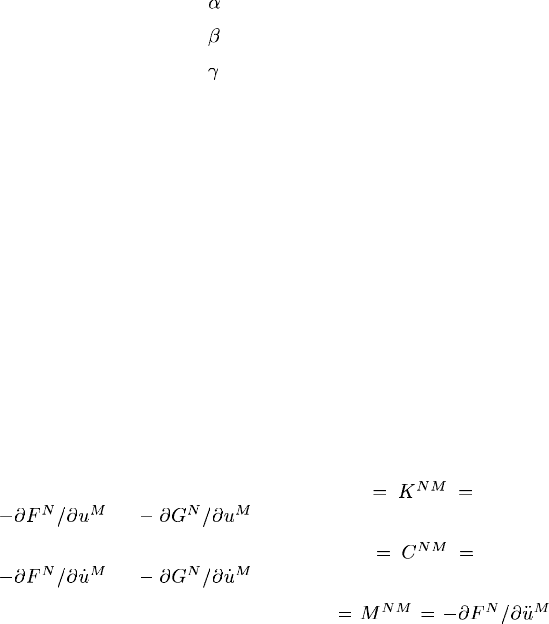
UEL
PREDEF(K1,K2,K3) Total or incremental value of t he K2th predefined field variable
at the K3th node of the element.
PREDEF(1,K2,K3) Values of the variables at the end of the current increment.
PREDEF(2,K2,K3) Incremental values corresponding to the current time
increment.
PARAMS
An array containing the parameters associated with the solution procedure. The entries in this array
depend on the solution procedure currently being use d when UEL is called, as indicated by the entries
in the LFLAGS array (see below).
For implicit dynam ics (LFLAGS(1) =11or12)PARAMS contains the integration operator values,
as:
PARAMS(1)
PARAMS(2)
PARAMS(3)
LFLAGS
An array containing the flags that defi ne the current solution procedure and requirements for element
calculations. Detailed requirements for the various Abaqus/Standard procedures are defined earlier in
this section.
LFLAGS(1) Defines the procedure type. See “Results file output format,” Section 5.1.2
of the Abaqus Analysis U ser’s Manual, for the key used for each
procedure.
LFLAGS(2)=0 Sm all-displacement analysis.
LFLAGS(2)=1 Large-displacement analysis (nonlinear geometric effects included in the
step; see “General and linear perturbation procedures,” Section 6.1.2 of
the Abaqus Analysis User’s Manual).
LFLAGS(3)=1 Norm al implicit time incrementation procedure. User subroutine UEL
must define the residual vector in RHS and the Jacobian matrix in AMATRX.
LFLAGS(3)=2
Define the current stiffness matrix (AMATRX
or )only.
LFLAGS(3)=3
Define the current damping matrix (AMATRX
or ) only.
LFLAGS(3)=4
Define the current mass matrix (AMATRX
)
only. Abaqus/Standard always requests an initial mass matrix at the start
of the analysis.
1.1.23–6
Abaqus ID:
Printed on:

UEL
LFLAGS(3)=5
Define the current residual or load vector (RHS
)only.
LFLAGS(3)=6 Define the current mass matrix and the residual vector for the initia l
acceleration calculation (or the calculation of accelerations after im pact).
LFLAGS(3)=100 Define perturbation quantities for output.
LFLAGS(4)=0 The step is a general step.
LFLAGS(4)=1 The step is a line ar perturbation step.
LFLAGS(5)=0
The current approximations to
, etc. were based on Newton
corrections.
LFLAGS(5)=1 The current approximations were found by extrapolation from the
previous increment.
TIME(1)
Current value of step time.
TIME(2)
Current value of total time.
Scalar parameters:
DTIME
Time increm ent.
PERIOD
Time period of the current s tep.
NDOFEL
Number of degrees of freedom in the elem ent.
MLVARX
Dimensioning parameter used when several displacement or right-hand-side vectors are used.
NRHS
Number of load vectors. NRHS is 1 in most nonlinear problems: it is 2 for the modified Riks static
procedure (“Static stress analysis,” Section 6.2.2 of the Abaqus Analysis User’s Manual), and it is
greater than 1 in some linear analysis procedures and during substructure generation.
NSVARS
User-defined number of solution- dependent state varia bles a ssociated wi th the element (“Defin ing
the number of solution-dependent variables that m ust be stored within the element” in “User-defined
elements,” Section 29.16.1 of the Abaqus Analysis User’s Manual).
1.1.23–7
Abaqus ID:
Printed on:
UEL
NPROPS
User-defined number of real property values associated with the element (“Defining the element
properties” in “User-defined elements,” Section 29.16.1 of the Abaqus Analysis User’s Manual).
NJPROP
User-defined num ber of integer property values associated with the element (“Defining the element
properties” in “User-defined elements,” Section 29.16.1 of the Abaqus Analysis User’s Manual).
MCRD
MCRD is defined as the maximum of the user-defined maximum number of coordinates needed at any
node point (“Defining the maxim um number of coordinates needed at any nodal point” in “User-defined
elements,” Section 29.16.1 of the Abaqus Analysis U ser’s Manual) and the value of the largest active
degree of freedom of the user elem ent that is less than or equal to 3. For example, if you specify that
the maximum num ber of coordinates is 1 and the active degrees of freedom of the user element are 2,
3, and 6, MCRD will be 3. If you specify that the maxim um number of coordinates is 2 and the active
degrees of freedom of the user e lement are 11 and 12, MCRD will be 2.
NNODE
User-defined num ber of nodes on the element (“Defining the number of nodes associated with the
element” in “User-defined elements,” Section 29.16.1 of the Abaqus A nalysis User’s Manual).
JTYPE
Integer defining the eleme nt ty pe. This is the user-defined integer value n in elem ent type
Un (“Assigning an element type key to a user-defined element” in “User-defined elements,”
Section 29.16.1 of the Abaqus Analysis User’s Manual).
KSTEP
Current step number.
KINC
Current increment number.
JELEM
User-assigned element num ber.
NDLOAD
Identification number of the distributed load or flux currently active on this element.
MDLOAD
Total number of distr ibuted loads and/or fluxes define d on this element.
NPREDF
Number of predefined field variables, including temperature. For user elements Abaqus/Standard uses
one value for each field variable per node.
1.1.23–8
Abaqus ID:
Printed on:

UEL
UEL conventions
The solution variables (displacement, velocity, etc.) are arranged on a node/degree of freedom basis.
The degrees of freedom of the first node are first, followed by the degrees of freedom of the second node,
etc.
Usage with general nonlinear procedures
The values of (and, in direct-integration dynamic steps, and ) enter user subroutine UEL as
their latest approximations at the end of the time increment; that is, at time
.
The values of
enter the subroutine as their values at the beginning of the time increment; t hat
is, a t tim e t. It is your responsibility to define suitable time integration schemes to update
.To
ensure accurate, stable integration of internal state variables, you can control the time incrementation via
PNEWDT.
The values of
enter the subroutine as the values of the total load magnitude for the th distrib uted
load at the end of the increment. Increments in the load magnitudes are also available.
In the following descriptions of the us er element’s requirements, it will be assumed that
LFLAGS(3)=1 unless otherwise stated.
Static analysis (LFLAGS(1)=1,2)
•
.
•
Automatic convergence checks are applied to the force residuals corresponding to degrees of
freedom 1–7.
•
You m us t d efin e AMATRX and RHS and update the state vari ables,
.
Modified Riks static analysis (LFLAGS(1)=1)and(NRHS=2)
•
,where , and are fixed load parameters, and is the
Riks (scalar) load parameter.
•
Automatic convergence checks are applied to the force residuals corresponding to degrees of
freedom 1–7.
•
You must defi ne AMATRX , RHS(1) ,andRHS(2)
and update the state variables, . RHS(2) is the incremental load vector.
Direct-integration dynamic analysis (LFLAGS(1)=11, 12)
•
Automatic convergence checks are applied to the force residuals corresponding to degrees of
freedom 1–7.
•
LFLAGS(3)=1: Normal time increment. Either the Hilber-Hughes-Taylor or the backward Euler
time integration scheme will be used. With
set to zero for the backward Euler, both schemes
imply
1.1.23–9
Abaqus ID:
Printed on:

UEL
where and ; that is,
the highest time derivative of
in and is ,sothat
Therefore, you must store as an internal state vector. If half-increment residual calculations
arerequired,youmustalsostore
as an internal state vector, where indicates the time at the
beginning of the previous increment . For
, and is not
needed. You m ust define AMATRX
where and . RHS must also be
defined and the state variables,
, updated. Although the value of given in the dynamic step
definitionispassedintoUEL, the value of
can vary from element to element. For example, can
be set to zero for som e elem ents in the model where numerical dissipation is not desired.
•
LFLAGS(3)=5: Half-increment residual ( ) calculation. A baqus/Standard will adjust the time
increment so that
(where is spec ified in the dynamic step
definition). The half-increment residu al is defined as
where indicates the time at the beginning of the previous increment ( is a param eter of the
Hilber-Hughes-Taylor time integration operator and will be set to zero if the backward Euler time
integration operator is used). You must define RHS
. To evaluate and ,you
must calculate
. These half-increment values will not be saved. DTIME will still contain
(not ). The values contained in U, V, A,andDU are half-increment values.
•
LFLAGS(3)=4: Velocity jum p calculation. Abaqus/Standard solves for ,
so y ou m ust define AMATRX
.
•
LFLAGS(3)=6: Initial acceleration calculation. Abaqus/Standard solves
for , so you must define AMATRX and RHS .
Subspace-based dynamic analysis (LFLAGS(1)=13)
•
The requirements are identical to those of static analysis, except that the Jacobian (stiffness),
AMATRX, is not needed. No convergence checks are performed in this case.
Quasi-static analysis (LFLAGS(1)=21)
•
The requirements are identical to those of static analysis.
1.1.23–10
Abaqus ID:
Printed on:

UEL
Steady-state heat transfer analysis (LFLAGS(1)=31)
•
The requirements are identical to those of static analysis, except that the autom atic convergence
checks are applied to the heat flux residuals corresponding to degrees of freedom 11, 12, …
Transient heat transfer analysis ( θ
max
)(LFLAGS(1)=32, 33)
•
Automatic convergence checks are applied to the heat flux residuals corresponding to degrees of
freedom 11, 12, …
•
The backward difference scheme is always used for tim e integration; that is, Abaqus/Standard
assumes that
,where and so always. For
degrees of freedom 11, 12, …,
will be compared against the user-prescribed maxim um
allowable nodal tem perature change in an increment,
, for controlling the time integration
accuracy.
•
You need to define AMATRX ,where is the heat capacity matrix and
RHS
, and must update the state variables, .
Geostatic analysis (LFLAGS(1)=61)
•
Identical to static analysis, except that the automatic convergence checks are applied to the residuals
corresponding to degrees of freedom 1–8 .
Steady-state coupled pore fluid diffusion/stress analysis (LFLAGS(1)=62, 63)
•
Identical to static analysis, except that the automatic convergence checks are applied to the residuals
corresponding to degrees of freedom 1–8 .
Transient coupled pore fluid diffusion/stress (consolidation) analysis ( u
w
max
)(LFLAGS(1)=64,
65)
•
Automatic convergence checks are a pplied to the re siduals corresponding to degrees of freed om
1–8.
•
The backward difference scheme is used for time integration; that is, ,where
.
•
For degree of freedom 8, will be compared against the user-prescribed maximum
wetting liquid pore pressure change,
, for automatic control of the time integration accuracy.
•
You m ust de fine AMATRX ,where is the pore fluid capacity matrix
and RHS
, and must update the st ate variables, .
Steady-state fully coupled thermal-stress analysis (LFLAGS(1)=71)
•
Identical to static analysis, except that the automatic convergence checks are applied to the residuals
corresponding to degrees of freedom 1–7 and 11, 12, …
1.1.23–11
Abaqus ID:
Printed on:

UEL
Transient fully coupled thermal-stress analysis (
θ
max
)(LFLAGS(1)=72,73)
•
Automatic convergence checks are a pplied to the re siduals corresponding to degrees of freed om
1–7 and 11, 12, …
•
Th
e backward difference scheme is used for time integration; that is,
,where
.
•
For degrees of freedom 11, 12, …, will be compared against the user-prescribed
maximum allowable noda l temperature change in an increment,
, for automatic control of
the time integration accuracy.
•
You m u st defin e AMATRX ,where is the heat capacity matrix and
RHS
, and must update the state variables, .
Steady-state coupled thermal-electrical analysis (LFLAGS(1)=75)
•
The requirements are identical to those of static analysis, except that the autom atic convergence
checks are applied to the c urrent density residuals corresponding to degree of freedom 9, in addition
to the heat flux residuals.
Transient coupled thermal-electrical analysis ( θ
max
)(LFLAGS(1)=76, 77)
•
Automatic convergence checks are applied to the current density residuals corresponding to degree
of freedom 9 and to the heat flux residuals corresponding to degree of freedom 11.
•
The backward difference scheme is always used for tim e integration; that is, Abaqus/Standard
assumes that
,where . Therefore, always. For
degree of freedom 11
will be compared against the user-prescribed maximum allowable
nodal temperature change in an increment,
, for controlling the time integration accuracy.
•
You m u st defin e AMATRX ,where is the heat capacity matrix and
RHS
, and must update the state variables, .
Usage with linear perturbation procedures
“General and linear perturbation procedures,” Section 6.1.2 of the Abaqus Analysis User’s Manual,
describes the linear perturbation capabilitie s in Abaqus/Standard. Here, base state values of var iables
will be denoted by
, , etc. Pe rturbation values will be denoted by , ,etc.
Abaqus/Standard will not call user subroutine UEL for the eigenvalue buckling prediction
procedure.
For response spectrum, random response, transient modal dynamic, and mode-based steady-state
dynamic procedures, user subroutine UEL is called only in a prior na tural frequency extraction analysis,
and the m ass and stiffness contributions are taken into account during modal superposition.
For direct-solution and mode-based steady-state dynamic, complex eigenvalue extraction, m atrix
generation, and substructure generation procedu res, Abaqus/Standard will call user subroutine UEL, but
only mass and stiffness contributions will be taken into account. The damping contributions will be
neglected.
1.1.23–12
Abaqus ID:
Printed on:

UEL
Static analysis (LFLAGS(1)=1, 2)
•
Abaqus/Standard will solve for ,where is the base state stiffness matrix
and the perturbation load vector,
, is a linear func tion of the perturbation loads, ; that is,
.
•
LFLAGS(3)=1: You must define AMATRX and RHS .
•
LFLAGS(3)=100: You must compute perturbations of the internal variables, , and define RHS
for output purposes.
Eigenfrequency extraction analysis (LFLAGS(1)=41)
•
.
•
Abaqus/Standard will solve for and ,where
is the base state stiffness matrix and is the base state mass
matrix.
•
LFLAGS(3)=2:DefineAMATRX .
•
LFLAGS(3)=4:DefineAMATRX .
Example: Structural and heat transfer user element
Both a structural and a heat transfer user element have been created to demonstrate the usage of subroutine
UEL. These user-defined elements are applied in a number of analyses. The following excerpt i s from
the verification problem that invokes the structural user elem ent in an im plicit dynamics procedure:
*
USER ELEMENT, NODES=2, TYPE=U1, PROPERTIES=4, COORDINATES=3,
VARIABLES=12
1, 2, 3
*
ELEMENT, TYPE=U1
101, 101, 102
*
ELGEN, ELSET=UTRUSS
101, 5
*
UEL PROPERTY, ELSET=UTRUSS
0.002, 2.1E11, 0.3, 7200.
The use r element cons ists of two nodes that are assumed to lie parallel to the x-axis. The element
behaves like a linear truss element. The supplied element properties ar e the cross-sectional area, Young’s
modulus, Poisson’s ratio, and dens ity, respectively.
The next excerpt shows the listing of the subroutine. The user subroutine has b een coded for use in
a perturbation static analysis; general static analysis, including Riks analysis with load incrementation
defined by the subroutine; eigenfrequency extraction analysis; and direct-integration dynamic analysis.
The nam es of the verification input files associated w ith the subroutine and these procedures can be found
in “UEL,” Section 4.1.14 of the Abaqus Verification Manual. The subroutine performs all calculations
required for the relevant procedures as described earlier in this section. The flags passed in through the
LFLAGS array are used to associate particular calculations with solution procedures.
1.1.23–13
Abaqus ID:
Printed on:
UEL
During a modified Riks analysis all force loads must be passed into UEL by means of distributed
load definitions such that they are available for the definition of incremental load vectors; the load keys
Un and UnNU must be used properly, a s discussed in “User-defined elements,” Sec tion 29.16.1 of the
Abaqus Analysis User’s Manual. The coding in subroutine UEL must distribute the loads into consistent
equivalent nodal forces and account for them in the calculation of the RHS and ENERGY arrays.
SUBROUTINE UEL(RHS,AMATRX,SVARS,ENERGY,NDOFEL,NRHS,NSVARS,
1 PROPS,NPROPS,COORDS,MCRD,NNODE,U,DU,V,A,JTYPE,TIME,
2 DTIME,KSTEP,KINC,JELEM,PARAMS,NDLOAD,JDLTYP,ADLMAG,
3 PREDEF,NPREDF,LFLAGS,MLVARX,DDLMAG,MDLOAD,PNEWDT,
4 JPROPS,NJPROP,PERIOD)
C
INCLUDE 'ABA_PARAM.INC'
PARAMETER ( ZERO = 0.D0, HALF = 0.5D0, ONE = 1.D0 )
C
DIMENSION RHS(MLVARX,*),AMATRX(NDOFEL,NDOFEL),
1 SVARS(NSVARS),ENERGY(8),PROPS(*),COORDS(MCRD,NNODE),
2 U(NDOFEL),DU(MLVARX,*),V(NDOFEL),A(NDOFEL),TIME(2),
3 PARAMS(3),JDLTYP(MDLOAD,*),ADLMAG(MDLOAD,*),
4 DDLMAG(MDLOAD,*),PREDEF(2,NPREDF,NNODE),LFLAGS(*),
5 JPROPS(*)
DIMENSION SRESID(6)
C
C UEL SUBROUTINE FOR A HORIZONTAL TRUSS ELEMENT
C
C SRESID - stores the static residual at time t+dt
C SVARS - In 1-6, contains the static residual at time t
C upon entering the routine. SRESID is copied to
C SVARS(1-6) after the dynamic residual has been
C calculated.
C - For half-increment residual calculations: In 7-12,
C contains the static residual at the beginning
C of the previous increment. SVARS(1-6) are copied
C into SVARS(7-12) after the dynamic residual has
C been calculated.
C
AREA = PROPS(1)
E = PROPS(2)
ANU = PROPS(3)
RHO = PROPS(4)
C
ALEN = ABS(COORDS(1,2)-COORDS(1,1))
AK = AREA*E/ALEN
1.1.23–14
Abaqus ID:
Printed on:
UEL
AM = HALF*AREA*RHO*ALEN
C
DO K1 = 1, NDOFEL
SRESID(K1) = ZERO
DO KRHS = 1, NRHS
RHS(K1,KRHS) = ZERO
END DO
DO K2 = 1, NDOFEL
AMATRX(K2,K1) = ZERO
END DO
END DO
C
IF (LFLAGS(3).EQ.1) THEN
C Normal incrementation
IF (LFLAGS(1).EQ.1 .OR. LFLAGS(1).EQ.2) THEN
C *STATIC
AMATRX(1,1) = AK
AMATRX(4,4) = AK
AMATRX(1,4) = -AK
AMATRX(4,1) = -AK
IF (LFLAGS(4).NE.0) THEN
FORCE = AK*(U(4)-U(1))
DFORCE = AK*(DU(4,1)-DU(1,1))
SRESID(1) = -DFORCE
SRESID(4) = DFORCE
RHS(1,1) = RHS(1,1)-SRESID(1)
RHS(4,1) = RHS(4,1)-SRESID(4)
ENERGY(2) = HALF*FORCE*(DU(4,1)-DU(1,1))
* + HALF*DFORCE*(U(4)-U(1))
* + HALF*DFORCE*(DU(4,1)-DU(1,1))
ELSE
FORCE = AK*(U(4)-U(1))
SRESID(1) = -FORCE
SRESID(4) = FORCE
RHS(1,1) = RHS(1,1)-SRESID(1)
RHS(4,1) = RHS(4,1)-SRESID(4)
DO KDLOAD = 1, NDLOAD
IF (JDLTYP(KDLOAD,1).EQ.1001) THEN
RHS(4,1) = RHS(4,1)+ADLMAG(KDLOAD,1)
ENERGY(8) = ENERGY(8)+(ADLMAG(KDLOAD,1)
* - HALF*DDLMAG(KDLOAD,1))*DU(4,1)
IF (NRHS.EQ.2) THEN
1.1.23–15
Abaqus ID:
Printed on:
UEL
C Riks
RHS(4,2) = RHS(4,2)+DDLMAG(KDLOAD,1)
END IF
END IF
END DO
ENERGY(2) = HALF*FORCE*(U(4)-U(1))
END IF
ELSE IF (LFLAGS(1).EQ.11 .OR. LFLAGS(1).EQ.12) THEN
C *DYNAMIC
ALPHA = PARAMS(1)
BETA = PARAMS(2)
GAMMA = PARAMS(3)
C
DADU = ONE/(BETA*DTIME**2)
DVDU = GAMMA/(BETA*DTIME)
C
DO K1 = 1, NDOFEL
AMATRX(K1,K1) = AM*DADU
RHS(K1,1) = RHS(K1,1)-AM*A(K1)
END DO
AMATRX(1,1) = AMATRX(1,1)+(ONE+ALPHA)*AK
AMATRX(4,4) = AMATRX(4,4)+(ONE+ALPHA)*AK
AMATRX(1,4) = AMATRX(1,4)-(ONE+ALPHA)*AK
AMATRX(4,1) = AMATRX(4,1)-(ONE+ALPHA)*AK
FORCE = AK*(U(4)-U(1))
SRESID(1) = -FORCE
SRESID(4) = FORCE
RHS(1,1) = RHS(1,1) -
* ((ONE+ALPHA)*SRESID(1)-ALPHA*SVARS(1))
RHS(4,1) = RHS(4,1) -
* ((ONE+ALPHA)*SRESID(4)-ALPHA*SVARS(4))
ENERGY(1) = ZERO
DO K1 = 1, NDOFEL
SVARS(K1+6) = SVARS(k1)
SVARS(K1) = SRESID(K1)
ENERGY(1) = ENERGY(1)+HALF*V(K1)*AM*V(K1)
END DO
ENERGY(2) = HALF*FORCE*(U(4)-U(1))
END IF
ELSE IF (LFLAGS(3).EQ.2) THEN
C Stiffness matrix
AMATRX(1,1) = AK
1.1.23–16
Abaqus ID:
Printed on:
UEL
AMATRX(4,4) = AK
AMATRX(1,4) = -AK
AMATRX(4,1) = -AK
ELSE IF (LFLAGS(3).EQ.4) THEN
C Mass matrix
DO K1 = 1, NDOFEL
AMATRX(K1,K1) = AM
END DO
ELSE IF (LFLAGS(3).EQ.5) THEN
C Half-increment residual calculation
ALPHA = PARAMS(1)
FORCE = AK*(U(4)-U(1))
SRESID(1) = -FORCE
SRESID(4) = FORCE
RHS(1,1) = RHS(1,1)-AM*A(1)-(ONE+ALPHA)*SRESID(1)
* + HALF*ALPHA*( SVARS(1)+SVARS(7) )
RHS(4,1) = RHS(4,1)-AM*A(4)-(ONE+ALPHA)*SRESID(4)
* + HALF*ALPHA*( SVARS(4)+SVARS(10) )
ELSE IF (LFLAGS(3).EQ.6) THEN
C Initial acceleration calculation
DO K1 = 1, NDOFEL
AMATRX(K1,K1) = AM
END DO
FORCE = AK*(U(4)-U(1))
SRESID(1) = -FORCE
SRESID(4) = FORCE
RHS(1,1) = RHS(1,1)-SRESID(1)
RHS(4,1) = RHS(4,1)-SRESID(4)
ENERGY(1) = ZERO
DO K1 = 1, NDOFEL
SVARS(K1) = SRESID(K1)
ENERGY(1) = ENERGY(1)+HALF*V(K1)*AM*V(K1)
END DO
ENERGY(2) = HALF*FORCE*(U(4)-U(1))
ELSE IF (LFLAGS(3).EQ.100) THEN
C Output for perturbations
IF (LFLAGS(1).EQ.1 .OR. LFLAGS(1).EQ.2) THEN
C *STATIC
FORCE = AK*(U(4)-U(1))
DFORCE = AK*(DU(4,1)-DU(1,1))
SRESID(1) = -DFORCE
SRESID(4) = DFORCE
1.1.23–17
Abaqus ID:
Printed on:
UEL
RHS(1,1) = RHS(1,1)-SRESID(1)
RHS(4,1) = RHS(4,1)-SRESID(4)
ENERGY(2) = HALF*FORCE*(DU(4,1)-DU(1,1))
* + HALF*DFORCE*(U(4)-U(1))
* + HALF*DFORCE*(DU(4,1)-DU(1,1))
DO KVAR = 1, NSVARS
SVARS(KVAR) = ZERO
END DO
SVARS(1) = RHS(1,1)
SVARS(4) = RHS(4,1)
ELSE IF (LFLAGS(1).EQ.41) THEN
C *FREQUENCY
DO KRHS = 1, NRHS
DFORCE = AK*(DU(4,KRHS)-DU(1,KRHS))
SRESID(1) = -DFORCE
SRESID(4) = DFORCE
RHS(1,KRHS) = RHS(1,KRHS)-SRESID(1)
RHS(4,KRHS) = RHS(4,KRHS)-SRESID(4)
END DO
DO KVAR = 1, NSVARS
SVARS(KVAR) = ZERO
END DO
SVARS(1) = RHS(1,1)
SVARS(4) = RHS(4,1)
END IF
END IF
C
RETURN
END
1.1.23–18
Abaqus ID:
Printed on:

UELMAT
1.1.24 UELMAT: User subroutine to define an element with access to Abaqus materials.
Product:
Abaqus/Standard
WARNING: This feature is intended f or advanced users only. Its use in all but the
simplest test examples will require considerable coding by the user/developer.
“User-defined elements,” Section 29.16.1 of the Abaqus Analysis User’s Manual,
should be read before proceeding.
References
•
“User-defined elements,” Section 29.16.1 of the Abaqus A nalysis User’s Manual
• *
UEL PROPERTY
• *
USER ELEMENT
•
“Accessing Abaqus materials,” Section 2.1.17
•
“Accessing Abaqus thermal materials,” Section 2.1.18
Overview
User subroutine UELMAT:
•
will be called for each element that is of a general user-defined elem ent type (i.e., not defined by
a linear stiffness or mass matrix read either directly or from results file data) each tim e element
calculations are required;
•
(or subroutines called by user subroutine UELMAT) must perform all of the calculations for the
element, appropriate to the current activity in the analysis;
•
can access some of the Abaqus m aterials through utility routines MATERIAL_LIB_MECH and
MATERIAL_LIB_HT;
•
is available for a subset of the procedures supported for user subroutine UEL (see “User-defined
elements,” Section 29.16.1 of the Abaqus Analysis User’s Manual); and
•
is available for plane stress and three-dimensional element types in a stress/displacement analysis
and for two-dimensional and three-dimensional elem ent types in a heat transfer analysis (see “User-
defined elements,” Section 29.16.1 of the Abaqus Analysis User’s Manual).
User subroutine interface
SUBROUTINE UELMAT(RHS,AMATRX,SVARS,ENERGY,NDOFEL,NRHS,NSVARS,
1 PROPS,NPROPS,COORDS,MCRD,NNODE,U,DU,V,A,JTYPE,TIME,DTIME,
2 KSTEP,KINC,JELEM,PARAMS,NDLOAD,JDLTYP,ADLMAG,PREDEF,NPREDF,
3 LFLAGS,MLVARX,DDLMAG,MDLOAD,PNEWDT,JPROPS,NJPROP,PERIOD,
4 MATERIALLIB)
1.1.24–1
Abaqus ID:
Printed on:

UELMAT
C
INCLUDE 'ABA_PARAM.INC'
C
DIMENSION RHS(MLVARX,*),AMATRX(NDOFEL,NDOFEL),PROPS(*),
1 SVARS(*),ENERGY(8),COORDS(MCRD,NNODE),U(NDOFEL),
2 DU(MLVARX,*),V(NDOFEL),A(NDOFEL),TIME(2),PARAMS(*),
3 JDLTYP(MDLOAD,*),ADLMAG(MDLOAD,*),DDLMAG(MDLOAD,*),
4 PREDEF(2,NPREDF,NNODE),LFLAGS(*),JPROPS(*)
user coding to define RHS, AMATRX, SVARS, ENERGY, and PNEWDT
RETURN
END
Variables to be defined
These arrays depend on the value of the LFLAGS array.
RHS
An array containing the contribu tions of this element to the right-hand- side vectors of the overa ll system
of equations. For most nonlinear analysis procedures, NRHS=1 and RHS should contain the residual
vector. The exception is the modified Riks static procedure (“Static stress analysis,” Section 6.2.2 of the
Abaqus Analysis User’s Manual), for which NRHS=2 and the first column in RHS should contain the
residual vector and the second column should contain the increments of external load on the elem ent.
RHS(K1,K2) is the entry for the K1th degree of freedom of the element in the K2th right-hand-side
vector.
AMATRX
An array containing the contribution of this element to the Jacobian (stiffness) o r other matrix of the
overall system of equations. The particular matrix required at any time depends on th e entries in the
LFLAGS array (see below).
All nonzero entries in AMATRX should be defined, even if the matrix is symme tric. If you do
not specify that the matrix is unsymmetric when you define the user element, Abaqus/Standard will
use the symmetri c ma trix defined by
,where is the m atrix defined as AMATRX
in this subroutine. If you specify that the matrix is unsymmetric when you define the user elem ent,
Abaqus/Standard will use AMATRX directly.
SVARS
An array containing the values of the solution-dependent state variables associated with this element.
The number of such variables is NSVARS (see below). You define the meaning of these variables.
For general nonlinear steps this array is passed into UELMAT containing the values of these
variables at the start of the current increment. They should be updated to be the values at the end
1.1.24–2
Abaqus ID:
Printed on:

UELMAT
of the increment, unless the procedure during which UELMAT is being called does not require such
an up date; this requirement depends on the entrie s in the LFLAGS array (see below). For linear
perturbation steps this array is passed into UELMAT containing the values of these variables in the base
state. They s hould be returned containing perturb ation values if you wish to output such quantities.
When KINC is equal to zero, the call to UELMAT is made for zero increment output (see “Output,”
Section 4.1.1 of the Abaqus Analysis User’s Manual). In this case the values returned will be used only
for output purposes and are not updated permanently.
ENERGY
For general nonlinear steps array ENERGY contains the values of the energy quantities associated with
the element. The values in this array when UELMAT is calle d are the element energy quantities at the
start of the current increment. They should be updated to the values at the end of the current incre ment.
For linear perturbation steps the array is passed into UELMAT containing the e nergy in the base st ate.
They should be returned containing perturbation values if you wish to output such quantities. The
entries in the array are as follows:
ENERGY(1) Kinetic ene rgy.
ENERGY(2) Elastic strain energy.
ENERGY(3) Creep dissipation.
ENERGY(4) Plastic dissi pation.
ENERGY(5) Viscous dissipation.
ENERGY(6) “Artificial strain energy” associated with such effects as artificial
stiffness introduced to control hourglassing or other singular modes
in the element.
ENERGY(7) Electrostatic energy.
ENERGY(8) Incremental work done by loads applied within the user element.
When KINC is equal to zero, the call to UELMAT is made for zero increment output (see “Output,”
Section 4.1.1 of the Abaqus Analysis User’s Manual). In this case the energy values returned will be
used only for output purposes and are not upda ted permanently.
Variable that can be updated
PNEWDT
Ratio of s uggested new time inc rement to the tim e increment currently being used (DTIME,see
below). This variable allows you to provide input to the automatic t ime incrementation algorithms in
Abaqus/Standard (if automatic time incrementation is chosen). It is useful only during equilibrium
iterations with the normal time incrementation, as indicated by LFLAGS(3)=1. During a severe
discontinuity iteration (such as contact changes), PNEWDT is ignored unless CONV ERT SDI=YES is
specified for this step. The usage of PNEWDT is discussed below.
PNEWDT is set to a large value before each call to UELMAT.
1.1.24–3
Abaqus ID:
Printed on:

UELMAT
If PNEWDT is redefined to be less than 1.0, Abaqus/Standard must abandon the time increment
and attem pt it again with a smaller time increment. The suggested new time increment provided to the
automatic time integration algorithms is PNEWDT × DTIME, wher e the PNEWDT used is the minimum
value for all calls to user subroutines that allow redefinition of PNEWDT for this iteration.
If PNEWDT is given a v alue that is greater than 1.0 for all calls to user subroutines for this iteration
and the increment converges in this iteration, A baqus/Standard m ay increase the time increment. The
suggested new time increment provided to the automatic time integration algorithms is PNEWDT ×
DTIME, where the PNEWDT used is the minimum value for all calls to user subroutines for this iteration.
If automatic time incrementation is not selected in the anal ysis proc edure, values of PNEWDT that
are greater than 1.0 will be ignored and values of PNEWDT that are less than 1.0 will cause the job to
terminate.
Variables passed in for information
Arrays:
PROPS
A floating point array containing the NPROPS real property values defined for use with this element.
NPROPS is the user-specified number of real property values. See “D efining the elem ent properties”
in “User-defined elements,” Section 29.16.1 of the Abaqus Analysis User’s Manual.
JPROPS
An integer array containing the NJPROP integer property values defined for use with this element.
NJPROP is the user-specified number of integer property values. See “Defining the element properties”
in “User-defined elements,” Section 29.16.1 of the Abaqus Analysis User’s Manual.
COORDS
An array containing the original coordinates of the nodes of the element. COORDS(K1,K2) is the
K1th coordinate of the K2th node of the element.
U, DU, V, A
Arrays containing the current estimates of the basic solution variables (displacements, rotations,
temperatures, depending on the degree of freedom) at the nodes of the element at the end of the
current increment. Values are provided as follows:
U(K1) Total values of the variabl es. If this is a linea r perturbation step, it is
the value in the base state.
DU(K1,KRHS) Incremental values of the variables for the current increment for
right-hand-side KRHS. If this is an eigenvalue extraction step, this is
the eigenvector magnitude for eigenvector KRHS. For steady-state
dynamics KRHS
denotes real components of perturbation
displacement and KRHS
denotes imaginary components of
perturbation displacement.
1.1.24–4
Abaqus ID:
Printed on:

UELMAT
V(K1) Time rate of change of the variables (velocities, rates of rotation).
Defined for implicit dynamics only (LFLAGS(1)
11 or 12).
A(K1) Accelerations of the variables. D efined for implicit dynamics only
(LFLAGS(1)
11 or 12).
JDLTYP
An array containing the integers used to define distributed load types for the elem ent. Loads of type
Un are identified by the integer value n in JDLTYP; loads of type UnNU are identified by the negative
integer value
in JDLTYP. JDLTYP(K1,K2) is the identifier of t he K1th distributed load in the
K2th load case. For general nonlinear steps K2 is always 1.
ADLMAG
For general nonlinear steps ADLMAG(K1,1) is the total load magnitude of the K1th distributed load at
the end of the current increment for distributed loads of type Un. For distributed loads of type UnNU,
the load magnitude is defined in UELMAT; t herefore, the corresponding entries in ADLMAG are zero.
For linear perturbation steps ADLMAG(K1,1) contains the total load ma gnitude of the K1th distributed
load of type U n applied in the base state. Base state loading of type U nNU m ust be dealt with inside
UELMAT. ADLMAG(K1,2), ADLMAG(K1,3), etc. are currently not used.
DDLMAG
For general nonlinear steps DDLMAG contains the incre ments in the magnitudes of the distributed loads
that are currently active on this element for distributed loads of type Un. DDLMAG(K1,1) is the
increment of magnitude of the load for the curre nt time increment. The increment of load magnitud e
is needed to compute the external work contribution. For distributed loads of type UnNU the load
magnitude is defined in UELMAT; therefore, the corre sponding entries in DDLMAG are zero. For linear
perturbation steps DDLMAG(K1,K2) contains the perturbation in the magnitudes of the distributed
loads that are currently active on this element for distributed loads of type U n. K1 den otes the K1th
perturbation load active on the elem ent. K2 is always 1, except for steady-state dynamics, w here K2=1
for real loads and K2=2 for imaginary loads. Pertur bation loads of type UnNU must be dealt with
inside UELMAT.
PREDEF
An array containing the values of predefined field variables, such as temperature in an uncoupled
stress/displacement analysis, at the nodes of the elem ent (“Predefined fields,” Section 30.6.1 of the
Abaqus Analysis User’s Manual).
The first index of the array, K1, is either 1 or 2, with 1 indicatin g the value of the field variable
at the end of the increment and 2 indicating the increment in the field variable. The second index,
K2, indicates the variable: the temperature corresponds to index 1, and the predefined field variables
correspond to indices 2 and above. In cases where temperature is not defined, the predefined field
variables begin with index 1. The third index, K3, indicates the local node number on the element.
1.1.24–5
Abaqus ID:
Printed on:

UELMAT
PREDEF(K1,1,K3) Tem perature.
PREDEF(K1,2,K3) First predefined field variable.
PREDEF(K1,3,K3) Second predefined field variable.
Etc. Any other predefined field variable.
PREDEF(K1,K2,K3) Total or incremental value of t he K2th predefined field variable
at the K3th node of the element.
PREDEF(1,K2,K3) Values of the variables at the end of the current increment.
PREDEF(2,K2,K3) Incremental values corresponding to the current time
increment.
PARAMS
An array containing the parameters associated with the solution procedure. The entries in this array
depend on the solution procedure currently being used when UELMAT is called, as indicated by the
entries in the LFLAGS array (see below).
For implicit dynam ics (LFLAGS(1) =11or12)PARAMS con tains the integration operator values,
as:
PARAMS(1)
PARAMS(2)
PARAMS(3)
LFLAGS
An array containing the flags that defi ne the current solution procedure and requirements for element
calculations. Detailed requirements for the various Abaqus/Standard procedures are defined earlier in
this section.
LFLAGS(1) Defines the procedure type. See “Results file output format,” Section 5.1.2
of the Abaqus Analysis U ser’s Manual, for the key used for each
procedure.
LFLAGS(2)=0 Sm all-displacement analysis.
LFLAGS(2)=1 Large-displacement analysis (nonlinear geometric effects included in the
step; see “General and linear perturbation procedures,” Section 6.1.2 of
the Abaqus Analysis User’s Manual).
LFLAGS(3)=1 Norm al implicit time incrementation procedure. User subroutine UELMAT
must define the residual vector in RHS and the Jacobian matrix in AMATRX.
LFLAGS(3)=2
Define the current stiffness matrix (AMATRX
or )only.
1.1.24–6
Abaqus ID:
Printed on:

UELMAT
LFLAGS(3)=3
Define the current damping matrix (AMATRX
or ) only.
LFLAGS(3)=4
Define the current mass matrix (AMATRX
)
only. Abaqus/Standard always requests an initial mass matrix at the start
of the analysis.
LFLAGS(3)=5
Define the current residual or load vector (RHS
)only.
LFLAGS(3)=6 Define the current mass matrix and the residual vector for the initia l
acceleration calculation (or the calculation of accelerations after im pact).
LFLAGS(3)=100 Define perturbation quantities for output.
LFLAGS(4)=0 The step is a general step.
LFLAGS(4)=1 The step is a line ar perturbation step.
LFLAGS(5)=0
The current approximations to
, etc. were based on Newton
corrections.
LFLAGS(5)=1 The current approximations were found by extrapolation from the
previous increment.
TIME(1)
Current value of step time.
TIME(2)
Current value of total time.
Scalar parameters:
DTIME
Time increm ent.
PERIOD
Time period of the current s tep.
NDOFEL
Number of degrees of freedom in the elem ent.
MLVARX
Dimensioning parameter used when several displacement or right-hand-side vectors are used.
NRHS
Number of load vectors. NRHS is 1 in most nonlinear problems: it is 2 for the modified Riks static
procedure (“Static stress analysis,” Section 6.2.2 of the Abaqus Analysis User’s Manual), and it is
greater than 1 in some linear analysis procedures and during substructure generation.
1.1.24–7
Abaqus ID:
Printed on:
UELMAT
NSVARS
User-defined number of solution- dependent state varia bles a ssociated wi th the element (“Defin ing
the number of solution-dependent variables that m ust be stored within the element” in “User-defined
elements,” Section 29.16.1 of the Abaqus Analysis User’s Manual).
NPROPS
User-defined number of real property values associated with the element (“Defining the element
properties” in “User-defined elements,” Section 29.16.1 of the Abaqus Analysis User’s Manual).
NJPROP
User-defined num ber of integer property values associated with the element (“Defining the element
properties” in “User-defined elements,” Section 29.16.1 of the Abaqus Analysis User’s Manual).
MCRD
MCRD is defined as the maximum of the user-defined maximum number of coordinates needed at any
node point (“Defining the maxim um number of coordinates needed at any nodal point” in “User-defined
elements,” Section 29.16.1 of the Abaqus Analysis U ser’s Manual) and the value of the largest active
degree of freedom of the user elem ent that is less than or equal to 3. For example, if you specify that
the maximum num ber of coordinates is 1 and the active degrees of freedom of the user element are 2,
3, and 6, MCRD will be 3. If you specify that the maxim um number of coordinates is 2 and the active
degrees of freedom of the user e lement are 11 and 12, MCRD will be 2.
NNODE
User-defined num ber of nodes on the element (“Defining the number of nodes associated with the
element” in “User-defined elements,” Section 29.16.1 of the Abaqus A nalysis User’s Manual).
JTYPE
Integer defining the eleme nt ty pe. This is the user-defined integer value n in elem ent type
Un (“Assigning an element type key to a user-defined element” in “User-defined elements,”
Section 29.16.1 of the Abaqus Analysis User’s Manual).
KSTEP
Current step number.
KINC
Current increment number.
JELEM
User-assigned element num ber.
NDLOAD
Identification number of the distributed load or flux currently active on this element.
MDLOAD
Total number of distr ibuted loads and/or fluxes define d on this element.
1.1.24–8
Abaqus ID:
Printed on:

UELMAT
NPREDF
Number of predefined field variables, including temperature. For user elements Abaqus/Standard uses
one value for each field variable per node.
MATERIALLIB
A variable that must be passed to the utility routines performing material point c omputations.
UELMAT conventions
The solution variables (displacement, velocity, etc.) are arranged on a node/degree of freedom basis.
The degrees of freedom of the first node are first, followed by the degrees of freedom of the second node,
etc.
Usage with general nonlinear procedures
The values of (and, in direct-integration dynamic steps, and ) enter user subroutine UELMAT
as their latest approximations at the end of the tim e increm ent; that is, at time
.
The values of
enter the subroutine as their values at the beginning of the time increment; t hat
is, a t tim e t. It is your responsibility to define suitable time integration schemes to update
.To
ensure accurate, stable integration of internal state variables, you can control the time incrementation via
PNEWDT.
The values of
enter the subroutine as the values of the total load magnitude for the th distrib uted
load at the end of the increment. Increments in the load magnitudes are also available.
In the following descriptions of the us er element’s requirements, it will be assumed that
LFLAGS(3)=1 unless otherwise stated.
Static analysis (LFLAGS(1)=1,2)
•
.
•
Automatic convergence checks are applied to the force residuals corresponding to degrees of
freedom 1–7.
•
You m us t d efin e AMATRX and RHS and update the state vari ables,
.
Direct-integration dynamic analysis (LFLAGS(1)=11, 12)
•
Automatic convergence checks are applied to the force residuals corresponding to degrees of
freedom 1–7.
•
LFLAGS(3)=1: Normal time increment. Either the Hilber-Hughes-Taylor or the backward Euler
time integration scheme will be used. With
set to zero for the backward Euler, both schemes
imply
1.1.24–9
Abaqus ID:
Printed on:

UELMAT
where and ; that is,
the highest time derivative of
in and is ,sothat
Therefore, you must store as an internal state vector. If half-increment residual calculations
arerequired,youmustalsostore
as an internal state vector, where indicates the time at the
beginning of the previous increment . For
, and is not
needed. You m ust define AMATRX
where and . RHS must also be
defined and the state variables,
, updated. Although the value of given in the dynamic step
definitionispassedintoUELMAT, the value of
can vary from element to elem ent. For example,
can be set to zero for some elem ents in the m odel where num erical dissipation is not desired.
•
LFLAGS(3)=5: Half-increment residual ( ) calculation. A baqus/Standard will adjust the time
increment so that
(where is spec ified in the dynamic step
definition). The half-increment residu al is defined as
where indicates the time at the beginning of the previous increment ( is a param eter of the
Hilber-Hughes-Taylor time integration operator and will be set to zero if the backward Euler time
integration operator is used). You must define RHS
. To evaluate and ,you
must calculate
. These half-increment values will not be saved. DTIME will still contain
(not ). The values contained in U, V, A,andDU are half-increment values.
•
LFLAGS(3)=4: Velocity jum p calculation. Abaqus/Standard solves for ,
so y ou m ust define AMATRX
.
•
LFLAGS(3)=6: Initial acceleration calculation. Abaqus/Standard solves
for , so you must define AMATRX and RHS .
Quasi-static analysis (LFLAGS(1)=21)
•
The requirements are identical to those of static analysis.
Steady-state heat transfer analysis (LFLAGS(1)=31)
•
The requirements are identical to those of static analysis, except that the autom atic convergence
checks are applied to the heat flux residuals corresponding to degrees of freedom 11, 12, …
Transient heat transfer analysis ( θ
max
)(LFLAGS(1)=32, 33)
•
Automatic convergence checks are applied to the heat flux residuals corresponding to degrees of
freedom 11, 12, …
1.1.24–10
Abaqus ID:
Printed on:

UELMAT
•
The backward difference scheme is always used for tim e integration; that is, Abaqus/Standard
assumes that
,where and so always. For
degrees of freedom 11, 12, …,
will be compared against the user-prescribed maxim um
allowable nodal tem perature change in an increment,
, for controlling the time integration
accuracy.
•
You need to define AMATRX ,where is the heat capacity matrix and
RHS
, and must update the state variables, .
Usage with linear perturbation procedures
“General and linear perturbation procedures,” Section 6.1.2 of the Abaqus Analysis User’s Manual,
describes the linear perturbation capabilitie s in Abaqus/Standard. Here, base state values of var iables
will be denoted by
, , etc. Pe rturbation values will be denoted by , ,etc.
Abaqus/Standard will not call user subroutine UELMAT for the following procedures: eigenvalue
buckling prediction, response spectrum, transient modal dynamic, steady-state dynam ic (modal and
direct), and random response.
Static analysis (LFLAGS(1)=1, 2)
•
Abaqus/Standard will solve for ,where is the base state stiffness matrix
and the perturbation load vector,
, is a linear func tion of the perturbation loads, ; that is,
.
•
LFLAGS(3)=1: You must define AMATRX and RHS .
•
LFLAGS(3)=100: You must compute perturbations of the internal variables, , and define RHS
for output purposes.
Eigenfrequency extraction analysis (LFLAGS(1)=41)
•
.
•
Abaqus/Standard will solve for and ,where
is the base state stiffness matrix and is the base state mass
matrix.
•
LFLAGS(3)=2:DefineAMATRX .
•
LFLAGS(3)=4:DefineAMATRX .
Example: Structural user element with Abaqus isotropic linearly elastic material
Both a structural and a heat transfer user element have been created to demonstrate the usage of subroutine
UELMAT. These user-defined elem ents are applied in a number of analyses. The following excerpt
illustrates how the linearly elastic isotropic material available in Abaqus can be accessed from user
subroutine UELMAT:
...
*
USER ELEMENT, TYPE=U1, NODES=4, COORDINATES=2, VAR=16,
INTEGRATION=4, TENSOR=PSTRAIN
1.1.24–11
Abaqus ID:
Printed on:
UELMAT
1,2
*
ELEMENT, TYPE=U1, ELSET=SOLID
1, 1,2,3,4
...
*
UEL PROPERTY, ELSET=SOLID, MATERIAL=MAT
...
*
MATERIAL, NAME=MAT
*
ELASTIC
7.00E+010, 0.33
The user element defi ned above is a 4-node, fully inte grated plane strain element, similar to the Abaqus
CPE4 element.
The next excerpt shows th
e listing of the user subroutine. I nside the subroutine, a loop over the
integration points is perfo
rmed. For each integration point the utility routine MATERIAL_LIB_MECH
is called, which returns stres
s and Jacobian at the integration point. These quantities are used to compute
the right-hand-side vector and th
e element Jacobian.
c***********************************************************
subroutine uelmat(rhs,amatrx,svars,energy,ndofel,nrhs,
1 nsvars,props,nprops,coords,mcrd,nnode,u,du,
2 v,a,jtype,time,dtime,kstep,kinc,jelem,params,
3 ndload,jdltyp,adlmag,predef,npredf,lflags,mlvarx,
4 ddlmag,mdload,pnewdt,jprops,njpro,period,
5 materiallib)
c
include 'aba_param.inc'
C
dimension rhs(mlvarx,*), amatrx(ndofel, ndofel), props(*),
1 svars(*), energy(*), coords(mcrd, nnode), u(ndofel),
2 du(mlvarx,*), v(ndofel), a(ndofel), time(2), params(*),
3 jdltyp(mdload,*), adlmag(mdload,*), ddlmag(mdload,*),
4 predef(2, npredf, nnode), lflags(*), jprops(*)
parameter (zero=0.d0, dmone=-1.0d0, one=1.d0, four=4.0d0,
1 fourth=0.25d0,gaussCoord=0.577350269d0)
parameter (ndim=2, ndof=2, nshr=1,nnodemax=4,
1 ntens=4, ninpt=4, nsvint=4)
c
c ndim ... number of spatial dimensions
c ndof ... number of degrees of freedom per node
c nshr ... number of shear stress component
c ntens ... total number of stress tensor components
c (=ndi+nshr)
1.1.24–12
Abaqus ID:
Printed on:
UELMAT
c ninpt ... number of integration points
c nsvint... number of state variables per integration pt
c (strain)
c
dimension stiff(ndof*nnodemax,ndof*nnodemax),
1 force(ndof*nnodemax), shape(nnodemax), dshape(ndim,nnodemax),
2 xjac(ndim,ndim),xjaci(ndim,ndim), bmat(nnodemax*ndim),
3 statevLocal(nsvint),stress(ntens), ddsdde(ntens, ntens),
4 stran(ntens), dstran(ntens), wght(ninpt)
c
dimension predef_loc(npredf),dpredef_loc(npredf),
1 defGrad(3,3),utmp(3),xdu(3),stiff_p(3,3),force_p(3)
dimension coord24(2,4),coords_ip(3)
data coord24 /dmone, dmone,
2 one, dmone,
3 one, one,
4 dmone, one/
c
data wght /one, one, one, one/
c
c*************************************************************
c
c U1 = first-order, plane strain, full integration
c
c State variables: each integration point has nsvint SDVs
c
c isvinc=(npt-1)*nsvint ... integration point counter
c statev(1+isvinc ) ... strain
c
c*************************************************************
if (lflags(3).eq.4) then
do i=1, ndofel
do j=1, ndofel
amatrx(i,j) = zero
end do
amatrx(i,i) = one
end do
goto 999
end if
c
c PRELIMINARIES
c
1.1.24–13
Abaqus ID:
Printed on:
UELMAT
pnewdtLocal = pnewdt
if(jtype .ne. 1) then
write(7,*)'Incorrect element type'
call xit
endif
if(nsvars .lt. ninpt*nsvint) then
write(7,*)'Increase the number of SDVs to', ninpt*nsvint
call xit
endif
thickness = 0.1d0
c
c INITIALIZE RHS AND LHS
c
do k1=1, ndof*nnode
rhs(k1, 1)= zero
do k2=1, ndof*nnode
amatrx(k1, k2)= zero
end do
end do
c
c LOOP OVER INTEGRATION POINTS
c
do kintk = 1, ninpt
c
c EVALUATE SHAPE FUNCTIONS AND THEIR DERIVATIVES
c
c determine (g,h)
c
g = coord24(1,kintk)*gaussCoord
h = coord24(2,kintk)*gaussCoord
c
c shape functions
shape(1) = (one - g)*(one - h)/four;
shape(2) = (one + g)*(one - h)/four;
shape(3) = (one + g)*(one + h)/four;
shape(4) = (one - g)*(one + h)/four;
c
c derivative d(Ni)/d(g)
dshape(1,1) = -(one - h)/four;
dshape(1,2) = (one - h)/four;
dshape(1,3) = (one + h)/four;
dshape(1,4) = -(one + h)/four;
1.1.24–14
Abaqus ID:
Printed on:
UELMAT
c
c derivative d(Ni)/d(h)
dshape(2,1) = -(one - g)/four;
dshape(2,2) = -(one + g)/four;
dshape(2,3) = (one + g)/four;
dshape(2,4) = (one - g)/four;
c
c compute coordinates at the integration point
c
do k1=1, 3
coords_ip(k1) = zero
end do
do k1=1,nnode
do k2=1,mcrd
coords_ip(k2)=coords_ip(k2)+shape(k1)*coords(k2,k1)
end do
end do
c
c INTERPOLATE FIELD VARIABLES
c
if(npredf.gt.0) then
do k1=1,npredf
predef_loc(k1) = zero
dpredef_loc(k1) = zero
do k2=1,nnode
predef_loc(k1) =
& predef_loc(k1)+
& (predef(1,k1,k2)-predef(2,k1,k2))*shape(k2)
dpredef_loc(k1) =
& dpredef_loc(k1)+predef(2,k1,k2)*shape(k2)
end do
end do
end if
c
c FORM B-MATRIX
c
djac = one
c
doi=1,ndim
doj=1,ndim
xjac(i,j) = zero
1.1.24–15
Abaqus ID:
Printed on:
UELMAT
xjaci(i,j) = zero
end do
end do
c
do inod= 1, nnode
do idim = 1, ndim
do jdim = 1, ndim
xjac(jdim,idim) = xjac(jdim,idim) +
1 dshape(jdim,inod)*coords(idim,inod)
end do
end do
end do
djac = xjac(1,1)*xjac(2,2) - xjac(1,2)*xjac(2,1)
if (djac .gt. zero) then
! jacobian is positive - o.k.
xjaci(1,1) = xjac(2,2)/djac
xjaci(2,2) = xjac(1,1)/djac
xjaci(1,2) = -xjac(1,2)/djac
xjaci(2,1) = -xjac(2,1)/djac
else
! negative or zero jacobian
write(7,*)'WARNING: element',jelem,'has neg.
1 Jacobian'
pnewdt = fourth
endif
if (pnewdt .lt. pnewdtLocal) pnewdtLocal = pnewdt
c
doi=1,nnode*ndim
bmat(i) = zero
end do
do inod = 1, nnode
do ider = 1, ndim
do idim = 1, ndim
irow = idim + (inod - 1)*ndim
bmat(irow) = bmat(irow) +
1 xjaci(idim,ider)*dshape(ider,inod)
end do
end do
end do
1.1.24–16
Abaqus ID:
Printed on:
UELMAT
c
c CALCULATE INCREMENTAL STRAINS
c
doi=1,ntens
dstran(i) = zero
end do
!
! set deformation gradient to Identity matrix
do k1=1,3
do k2=1,3
defGrad(k1,k2) = zero
end do
defGrad(k1,k1) = one
end do
c
c COMPUTE INCREMENTAL STRAINS
c
do nodi = 1, nnode
incr_row = (nodi - 1)*ndof
doi=1,ndof
xdu(i)= du(i + incr_row,1)
utmp(i) = u(i + incr_row)
end do
dNidx = bmat(1 + (nodi-1)*ndim)
dNidy = bmat(2 + (nodi-1)*ndim)
dstran(1) = dstran(1) + dNidx*xdu(1)
dstran(2) = dstran(2) + dNidy*xdu(2)
dstran(4) = dstran(4) +
1 dNidy*xdu(1) +
2 dNidx*xdu(2)
c deformation gradient
defGrad(1,1) = defGrad(1,1) + dNidx*utmp(1)
defGrad(1,2) = defGrad(1,2) + dNidy*utmp(1)
defGrad(2,1) = defGrad(2,1) + dNidx*utmp(2)
defGrad(2,2) = defGrad(2,2) + dNidy*utmp(2)
1.1.24–17
Abaqus ID:
Printed on:
UELMAT
end do
c
c CALL CONSTITUTIVE ROUTINE
c
isvinc= (kintk-1)*nsvint ! integration point increment
c
c prepare arrays for entry into material routines
c
doi=1,nsvint
statevLocal(i)=svars(i+isvinc)
end do
c
c state variables
c
do k1=1,ntens
stran(k1) = statevLocal(k1)
stress(k1) = zero
end do
c
do i=1, ntens
do j=1, ntens
ddsdde(i,j) = zero
end do
ddsdde(i,j) = one
enddo
c
c compute characteristic element length
c
celent = sqrt(djac*dble(ninpt))
dvmat = djac*thickness
c
dvdv0 = one
call material_lib_mech(materiallib,stress,ddsdde,
1 stran,dstran,kintk,dvdv0,dvmat,defGrad,
2 predef_loc,dpredef_loc,npredf,celent,coords_ip)
c
do k1=1,ntens
statevLocal(k1) = stran(k1) + dstran(k1)
end do
c
1.1.24–18
Abaqus ID:
Printed on:
UELMAT
isvinc= (kintk-1)*nsvint ! integration point increment
c
c update element state variables
c
doi=1,nsvint
svars(i+isvinc)=statevLocal(i)
end do
c
c form stiffness matrix and internal force vector
c
dNjdx = zero
dNjdy = zero
doi=1,ndof*nnode
force(i) = zero
doj=1,ndof*nnode
stiff(j,i) = zero
end do
end do
dvol= wght(kintk)*djac
do nodj = 1, nnode
incr_col = (nodj - 1)*ndof
dNjdx = bmat(1+(nodj-1)*ndim)
dNjdy = bmat(2+(nodj-1)*ndim)
force_p(1) = dNjdx*stress(1) + dNjdy*stress(4)
force_p(2) = dNjdy*stress(2) + dNjdx*stress(4)
do jdof = 1, ndof
jcol = jdof + incr_col
force(jcol) = force(jcol) +
& force_p(jdof)*dvol
end do
do nodi = 1, nnode
incr_row = (nodi -1)*ndof
dNidx = bmat(1+(nodi-1)*ndim)
1.1.24–19
Abaqus ID:
Printed on:
UELMAT
dNidy = bmat(2+(nodi-1)*ndim)
stiff_p(1,1) = dNidx*ddsdde(1,1)*dNjdx
& + dNidy*ddsdde(4,4)*dNjdy
& + dNidx*ddsdde(1,4)*dNjdy
& + dNidy*ddsdde(4,1)*dNjdx
stiff_p(1,2) = dNidx*ddsdde(1,2)*dNjdy
& + dNidy*ddsdde(4,4)*dNjdx
& + dNidx*ddsdde(1,4)*dNjdx
& + dNidy*ddsdde(4,2)*dNjdy
stiff_p(2,1) = dNidy*ddsdde(2,1)*dNjdx
& + dNidx*ddsdde(4,4)*dNjdy
& + dNidy*ddsdde(2,4)*dNjdy
& + dNidx*ddsdde(4,1)*dNjdx
stiff_p(2,2) = dNidy*ddsdde(2,2)*dNjdy
& + dNidx*ddsdde(4,4)*dNjdx
& + dNidy*ddsdde(2,4)*dNjdx
& + dNidx*ddsdde(4,2)*dNjdy
do jdof = 1, ndof
icol = jdof + incr_col
do idof = 1, ndof
irow = idof + incr_row
stiff(irow,icol) = stiff(irow,icol) +
& stiff_p(idof,jdof)*dvol
end do
end do
end do
end do
c
c assemble rhs and lhs
c
do k1=1, ndof*nnode
rhs(k1, 1) = rhs(k1, 1) - force(k1)
do k2=1, ndof*nnode
amatrx(k1, k2) = amatrx(k1, k2) + stiff(k1,k2)
end do
end do
end do ! end loop on material integration points
1.1.24–20
Abaqus ID:
Printed on:
UELMAT
pnewdt = pnewdtLocal
c
999 continue
c
return
end
1.1.24–21
Abaqus ID:
Printed on:

UEXPAN
1.1.25 UEXPAN: User subroutine to define incremental thermal strains.
Product:
Abaqus/Standard
References
•
“Thermal expansion,” Section 23.1.2 of the Abaqus Analysis User’s Manual
• *
EXPAN SION
•
“UEXPAN,” Section 4.1.16 of the A baqus Verification Manual
Overview
User subroutine UEXPAN:
•
can be used to define incremental thermal strains as functions of temperature, predefined field
variables, and state variables;
•
is intended for models in which the thermal strains depend on temperature and/or prede fined field
variables in complex ways or depend on state variables, which can be used and updated in this
routine;
•
is called at all integration points of elements for which the material or gasket behavior definition
contains user-subroutine-defined thermal expansion; and
•
is called twice per material point in each iteration during coupled temperature-displacement
analysis.
User subroutine interface
SUBROUTINE UEXPAN(EXPAN,DEXPANDT,TEMP,TIME,DTIME,PREDEF,
1 DPRED,STATEV,CMNAME,NSTATV,NOEL)
C
INCLUDE 'ABA_PARAM.INC'
C
CHARACTER*80 CMNAME
C
DIMENSION EXPAN(*),DEXPANDT(*),TEMP(2),TIME(2),PREDEF(*),
1 DPRED(*),STATEV(NSTATV)
user coding to define EXPAN, DEXPANDT and upda te
STATEV if necessary.
RETURN
END
1.1.25–1
Abaqus ID:
Printed on:

UEXPAN
Variables to be defined
EXPAN(*)
Increments of thermal strain. The number of values to be defined and the order in which they are
arranged depend on the type of thermal expansion being defined.
•
For isotropic expansion give the isotropic thermal stra in increment as the first and only component
of the matrix.
•
For orthotropic expansion give , ,and as the first, sec ond, and third components
of the matrix, respectively.
•
For anisotropic expansion give , , , , ,and . Direct components are
stored first, followed by shear components in the order presented here. For plane stress only three
components of the matrix are needed; give
, ,and , as the first, second, and third
components, respectively.
DEXPANDT(*)
Variation of therm al strains with respect to temperature,
. The number of values and the orde r
in which they are arranged depend on the type of thermal expansion being defined.
•
For isotropic expansion give the variation of the isotropic thermal stra in with respect to
temperature as the first and only component of the matrix.
•
For orthotropic expansion give , ,and as the first, second, and third
components of the matrix, respectively.
•
For anisotropic expansion give , , , , ,and .
Direct components are stored first, followed by shear components in the order presented here.
For plane stress only three components of the matrix are needed; give
, ,and
, as the first, second, and third components, respectively.
Variable that can be updated
STATEV(NSTATV)
Array containing the user-defined solution-dependent state variables at this point. Except for coupled
temperature-displacement analysis, these are supplied as values at the start of the increment and can
be updated to their values at the end of the increm ent. For coupled temperature-displacement analysis,
UEXPAN is called twice per material point per iteration. In the first call for a given material point and
iteration, the values supplied are those at the start of the increment and can be updated. In the second
call for the same material point and iteration, the values supplied are those returned from the first call,
and they can be updated again to their values at the end of the increment.
User subroutine UEXPAN allows for the incremental thermal strains to be only weakly dependent
on the state variables. The Jacobia n terms arising from the derivatives of the thermal strains with
respect to the state variables are not taken into account.
1.1.25–2
Abaqus ID:
Printed on:

UEXPAN
Variables passed in for information
TEMP(1)
Current temperature (at the end of the increment).
TEMP(2)
Tem perature increment.
TIME(1)
Step time at the end of the increment.
TIME(2)
Total time at the end of the increment.
DTIME
Time increm ent.
PREDEF(*)
Array containing the values of all the user-specified predefined field variables at this point (initial values
at the beginning of the analysis and current values during the analysis).
DPRED(*)
Array of increments of predefined field variables.
CMNAME
User-specified material name or gasket behavior name, left justified.
NSTATV
Number of solution-dependent state variables a ssociated with this material or gasket behavior
type (specified when space is allocated for the array; see “Allocating space” in “User subroutines:
overview,” Section 15.1.1 of the Abaqus Analysis User’s Manual).
NOEL
User-defined elem ent num ber.
1.1.25–3
Abaqus ID:
Printed on:

UEXTERNALDB
1.1.26 UEXTERNALDB: User subroutine to manage user-defined external databases and
calculate model-independent history information.
Product:
Abaqus/Standard
Reference
•
“User subroutines: overview,” Section 15.1.1 of the Abaqus Analysis User ’s Manual
Overview
User subroutine UEXTERNALDB:
•
is called once each at the beginning of the analysis, at the beginning of each increment, at the end
of each increm ent, and at the end of the analysis (in addition, the subroutine is also called once at
the beginning of a restart analysis);
•
can be used to com municate between other software and user subroutines within A baqus/Standard;
•
can be used to open external files needed for other user subroutines at the beginning of the analysis
and to close those files at the end of the analysis;
•
can be used to calculate or read history information at the beginning of each increment. This
information can be written to user-defined COMMON block variables or external files for use during
the analysis by other user subroutines; and
•
can be used to write the current values of the user-calculated history information to external files.
User subroutine interface
SUBROUTINE UEXTERNALDB(LOP,LRESTART,TIME,DTIME,KSTEP,KINC)
C
INCLUDE 'ABA_PARAM.INC'
C
DIMENSION TIME(2)
C
user coding to set up the FORTRAN environment, open files, close files,
calculate user-defined model-independent history information,
write history information to external files,
recover history information during restart a nalyses, etc.
do not include calls to utility routine XIT
RETURN
END
1.1.26–1
Abaqus ID:
Printed on:

UEXTERNALDB
Variable to be defined
None.
Variables passed in for information
LOP
LOP=0 indicates that the subroutine is being called at the start of the analysis.
LOP=1 indicates that the subroutine is being called at the start of the current analysis increment.
The subroutine can be called multiple tim es at the beginning of an analysis increment if the increment
fails to converge and a smaller time increment is required.
LOP=2 indicates that the subroutine is being called at the end of the current analysis increment.
When LOP=2, all information that you need to restart the analysis should be written to external files.
LOP=3 indicates that the subroutine is being called at the end of the analysis.
LOP=4 indicates that the subroutine is being called at the beginning of a restart analysis. When
LOP=4, all necessary external files should be opened and properly positioned and all information
required for the restart should be read from the externa l files.
LRESTART
LRESTART=0 indicates that an analysis restart file is not being written for this increment.
LRESTART=1 indicates that an analysis restart file is being written for this increment.
LRESTART=2 indicates that an analysis restart file is being written for this increment and that
only one increm ent is being retained per step so that the current increment overwrites the previous
increment in the restart file (see “Restarting an analysis,” Section 9.1.1 of the Abaqus Analysis User’s
Manual).
TIME(1)
Value of current step time.
TIME(2)
Value of current total time.
DTIME
Time increm ent.
KSTEP
Current step number. Whe n LOP=4, KSTEP gives the restart step number.
KINC
Current increment number. When LOP=4, KINC gives the restart increment num ber.
1.1.26–2
Abaqus ID:
Printed on:

UFIELD
1.1.27 UFIELD: User subroutine to specify predefined field variables.
Product:
Abaqus/Standard
References
•
“USDFLD,” Section 1.1.45
•
“Predefined fields,” Section 30.6.1 of the Abaqus Analysis User’s Manual
• *
FIELD
•
“UTEMP, UFIELD, UMASFL,andUPRESS,” Section 4.1.25 of the Abaqus Verification Manual
Overview
User subroutine UFIELD:
•
allows you to prescribe predefined field variables at the nodes of a m odel—the predefined field
variables at a node can be updated individually, or a number of field variables at the node can be
updated simultaneously;
•
is called whenever a user-subrout ine-defined field appears;
•
ignores any field variable values specified directly;
•
can be used to m odify field variable values read from a results file; and
•
can be used in conjunction with user subr outine USDFLD such that the field variables that are passed
in from UFIELD and interpolated to the material points can be modified (such changes are local to
material point values, and nodal field variable values remain unaffected).
Updating field variables
Two different methods are provided for updatin g field variables.
Individual variable updates
By default, only one field variable at a time can be updated in user subroutine UFIELD. In this case the
user subroutine will be called whenever a current value of a field variable is needed for a node that is
listed in the specified field variable definition. This m ethod can be used only for cases in which the field
variables are independent of each other.
Simultaneous variable updates
For cases in which the field variables depend on each other, m ultiple (possibly all) field variables at
a point can be updated simult aneously in user subroutine UFIELD. In this case you m ust specify the
number of field variables to be updated sim ultaneously at a point, and the user subroutine w ill be called
each time the current field variable values are needed.
1.1.27–1
Abaqus ID:
Printed on:

UFIELD
User subroutine interface
SUBROUTINE UFIELD(FIELD,KFIELD,NSECPT,KSTEP,KINC,TIME,NODE,
1 COORDS,TEMP,DTEMP,NFIELD)
C
INCLUDE 'ABA_PARAM.INC'
C
DIMENSION FIELD(NSECPT,NFIELD), TIME(2), COORDS(3),
1 TEMP(NSECPT), DTEMP(NSECPT)
C
user coding to define FIELD
RETURN
END
Variable to be defined
FIELD(NSECPT,NFIELD)
Array of predefined field variable values at node number NODE. When updating only one field
variable at a time, only the value of the specified field variable (see KFIELD below) must be returned.
In this case NFIELD is passed into user subroutine UFIELD with a value of 1, and FIELD is
thus dimensioned as FIELD(NSECPT,1). When updating all field variables s imultaneously, the
values of the specified number of field variables at the point must be returned. In this case FIELD
is dimensioned as FIELD(NSECPT,NFIELD),whereNFIELD is the number of field variables
specified and KFIELD has no meaning.
If NODE is part of any element other than a beam or shell, only one value of each field variable
must be returned (NSECPT=1). Otherwise, the num ber of values to be returned depends on the mode
of tem perature and field variable input selected for the beam or shell section. The following cases are
possible:
1. Temperatures and field variables for a beam section are given as values at the points shown in
the beam section descriptions. The number of values required, NSECPT, is determined by the
particular section type specified, as described in “B eam cross-section library,” Section 26.3.9 of
the Abaqus Analysis User’s Manual.
2. Temperatures and field variables are given as values at n equally spaced points through each layer
of a shell section. The number of values required, NSECPT,isequalton.
3. Temperatures and field variables for a beam section are given as values at the origin of the cross-
section together with gradients with respect to the 2-direction and, for three-dimensional beams,
the 1-direction of the section; or temperatures and field variables for a shell section are given
1.1.27–2
Abaqus ID:
Printed on:

UFIELD
as values at the reference surface together with gradients through the thickness. The number of
values required, NSECPT, is 3 for three-dimensional beams, 2 for two-dimensional beams, and 2
for shells. Give the midsurface value first, followed by the firs t and (if necessary) second gradients,
as described in “Beam elem ents,” Section 26.3 of the Abaqus Analysis User’s Manual, and “Shell
elements,” Section 26.6 of the Abaqus Analysis User’s Manual.
Since field variables can also be defined direc tly, it is important to understand the hierarchy used
in situations of conflicting information (see “Predefined fields,” Section 30.6.1 of the Abaqus A nalysis
User’s M anual).
When the array FIELD is passed into user subroutine UFIELD, it will contain either the field
variable values from the pre vious increment or those values obtained from the results file if this method
was used. You are then free to m odify these values within this subroutine.
Variables passed in for information
KFIELD
User-specified field variable number. This variable is meaningful only when updating individual field
variables at a time.
NFIELD
User-specified number of field variable s to be updated. This variable is meaningful only when updat ing
multiple field variables simultaneously.
NSECPT
Maximum number of sectio n values required for any node in the model. The NSECPT can be 2 when
only one field variable is specified at some non-beam or non-shell nodes in the model with conta ct.
KSTEP
Step number.
KINC
Increment number.
TIME(1)
Current value of step time.
TIME(2)
Current total tim e.
NODE
Node number.
COORDS
An array containing the coordinates of this node. These are the current coordinates if geometric
nonlinearity is accounted for during the step (see “Procedures: overview,” Section 6.1.1 of the Abaqus
Analysis User’s Manual); otherwise, the array contains the original coordinates of the node.
1.1.27–3
Abaqus ID:
Printed on:
UFIELD
TEMP(NSECPT)
Current tem perature at the node. If user subroutines UTEMP and UFIELD are both used, user subroutine
UTEMP is processed before user subroutine UFIELD.
DTEMP(NSECPT)
Tem perature increment at the node.
1.1.27–4
Abaqus ID:
Printed on:

UFLUID
1.1.28 UFLUID: User subroutine to define fluid density and fluid compliance for
hydrostatic fluid elements.
Product:
Abaqus/Standard
References
•
“Hydrostatic fluid models,” Section 23.4.1 of the Abaqus Analysis User’s Manual
• *
FLUID PROPERTY
•
“UFLUID,” Section 4.1.17 of the A baqus Verification Manual
Overview
User subroutine UFLUID:
•
is called for each cavity for which a user-defined fluid constitutive model is being specified;
•
is called for ev ery fluid element (“Hydrostatic fluid e lements,” Section 29.8.1 of the Abaqus
Analysis User’s Manual) and for every fluid link element (“Fluid link elements,” Section 29.8.3 of
the Abaqus A nalysis User’s Manual) connected to a cavity reference node;
•
requires that the fluid density, , and the fluid pre ssure compliance, ,bedefined;
•
requires that the fluid temperature compliance, ,bedefinediftheroutineistobeusedinalinear
perturbation step and the fluid is subjected to a temperature excursion; and
•
ignores any data specified for the fluid constitutive model outside the user subroutine.
Density and fluid mass
At the start of the analysis (prior to the first iteration) the density calculated in user subroutine UFLUID
(for the initial pressure,
, and temperature, ) is used to calculate the fluid mass from the initial cavity
volume. During the analysis the expected cavity volume is calculated from the fluid m ass and the density.
User subroutine interface
SUBROUTINE UFLUID(RHO,CP,CT,PNEWDT,ENER,PRESS,DPRESS,PRESSI,
1 TEMP,DTEMP,TEMPI,TIME,DTIME,KSTEP,KINC,NONUM,FLNAME,LFLAG)
C
INCLUDE 'ABA_PARAM.INC'
C
CHARACTER*80 FLNAME
DIMENSION TIME(2)
user coding to define RHO, CP, and CT
RETURN
END
1.1.28–1
Abaqus ID:
Printed on:

UFLUID
Variables to be defined
RHO
Fluid density,
, at the end of the increment.
CP
Fluid pressure compliance,
, at the end of the increment. For a linear perturbation step this is the
base state compliance. Fluid pressure complia nce is defined as
where p is the fluid cavity pressure.
CT
Fluid temperature compliance,
. This variable is needed only if a fluid tem perature excursion occurs
in a linear perturbation step and is the base state compliance. Fluid temperature comp liance is defined
as
where is the fluid cavity temperature.
Variables that can be updated
PNEWDT
Ratio of suggested new time increment to the time increment being used (DTIME, see below).
This variable allows you to provide input to the automatic time incrementation algorithms in
Abaqus/Standard (if automatic time incrementation is chosen).
PNEWDT is set to a large value before each call to UFLUID.
If PNEWDT is redefined to be less than 1.0, Abaqus/Standard must abandon the time increment
and attem pt it again with a smaller time increment. The suggested new time increment provided to the
automatic time integration algorithms is PNEWDT × DTIME, wher e the PNEWDT used is the minimum
value for all calls to user subroutines that allow redefinition of PNEWDT for this iteration.
If PNEWDT is given a v alue that is greater than 1.0 for all calls to user subroutines for this iteration
and the increment converges in this iteration, A baqus/Standard m ay increase the time increment. The
suggested new time increment provided to the automatic time integration algorithms is PNEWDT ×
DTIME, where the PNEWDT used is the minimum value for all calls to user subroutines for this iteration.
If automatic time incrementation is not selected in the anal ysis proc edure, values of PNEWDT that
are greater than 1.0 will be ignored and values of PNEWDT that are less than 1.0 will cause the job to
terminate.
ENER
Energy per unit mass stored in the fluid. This variable is used for energy output only and has no effect
on the solution.
1.1.28–2
Abaqus ID:
Printed on:

UFLUID
Variables passed in for information
PRESS
Fluid cavity pressure at the end of the increm ent. For a linear perturbation step this is the base state
pressure.
DPRESS
Fluid cavity pressure increment. For a linear perturbati on step this value is zero.
PRESSI
Fluid cavity pressure at the beginning of the analysis.
TEMP
Fluid cavity temperature at the end of the increment. For a linear perturbation step this is the base state
temperature.
DTEMP
Fluid cavity temperature increment. For a linear perturbation step this value is zero.
TEMPI
Fluid cavity temperature at the beginning of the analysis.
TIME(1)
Current value of step time at the start of the increment.
TIME(2)
Current value of total time at the start of the increment.
DTIME
Time increm ent.
KSTEP
Step number.
KINC
Increment number.
NONUM
Cavity reference node number.
FLNAME
User-specified fluid property nam e, left justified.
1.1.28–3
Abaqus ID:
Printed on:
UFLUID
LFLAG
Linear perturbation flag for the step. If this is a linear perturbation step, LFLAG=1. For a general
analysis step LFLAG=0.
1.1.28–4
Abaqus ID:
Printed on:

UFLUIDLEAKOFF
1.1.29 UFLUIDLEAKOFF: User subroutine to define the fluid leak-off coefficients for pore
pressure cohesive elements.
Product:
Abaqus/Standard
References
•
“Defining the constitutive response of fluid within the cohesive element gap,” Section 29.5.7 of the
Abaqus Analysis User’s Manual
• *
FLUID LEAKOFF
•
“Propagation of hydraulically driven fracture,” Section 3.3.2 of the Abaqus Verification Manual
Overview
User subroutine UFLUIDLEAKOFF:
•
can be used to define the fluid leak-off coefficients for pore pressure cohesive elements;
•
is called at all material calculation points of elements for which the m aterial definition contains
user-defined leak-off coefficients; and
•
can include material behavior dependent on field variables or state variables.
User subroutine interface
SUBROUTINE UFLUIDLEAKOFF(PERM,PGRAD,DN,P_INT,P_BOT,P_TOP,
1 ANM,TANG,TIME,DTIME,TEMP,DTEMP,PREDEF,DPRED,C_BOT,C_TOP,
2 DC_BOT,DC_TOP,STATEV,NSTATV,NOEL,NPT,KSTEP,KINC)
C
INCLUDE 'ABA_PARAM.INC'
C
CHARACTER*80 CMNAME
DIMENSION PERM(2),PGRAD(2),ANM(3),TANG(3,2),TIME(2),PREDEF(1),
1 DPRED(1),DC_BOT(3),DC_TOP(3),STATEV(NSTATV)
user coding to define C_BOT, C_TOP, DC_BOT, and DC_TOP
RETURN
END
1.1.29–1
Abaqus ID:
Printed on:

UFLUIDLEAKOFF
Variables to be defined
C_BOT
, fluid leak-off coefficient on the bottom side of a pore pressure cohesive element.
C_TOP
, fluid leak-off coefficient on the top side of a pore pressure cohesive element.
DC_BOT(1)
,whered=DN.
DC_BOT(2)
,where = P_INT.
DC_BOT(3)
,where =P_BOT.
DC_TOP(1)
,whered=DN.
DC_TOP(2)
,where = P_INT.
DC_TOP(3)
,where =P_TOP.
STATEV(NSTATV)
An array containing the values of the solution-dep endent state variables. You define the meaning of
these variables. These are passed in as the values at the beginning of the increment and must be returned
as the values at the end of the increment. The size of the array is defined as described in “Allocating
space” in “User subroutines: overview,” Section 15.1.1 of the Abaqus A nalysis User’s Manual.
Variables passed in for information
PERM(1)
Fluid permeability.
PERM(2)
The derivative of fluid permeability with regard to the opening.
PGRAD(1)
The first component of internal pressure gradient.
PGRAD(2)
The second component of internal pressure gradient.
1.1.29–2
Abaqus ID:
Printed on:
UFLUIDLEAKOFF
DN
The relative opening of the elem ent.
P_INT
Internal pressure.
P_BOT
Bottom pressure.
P_TOP
Top pressure.
ANM
Normal vector directed from the bottom face toward the top face.
TANG
Tangent direction vectors.
TIME(1)
Value of step time at the beginning of the current increment.
TIME(2)
Value of total tim e at the beginning of the current increment.
DTIME
Time increm ent.
TEMP
Tem perature at the start of the increment.
DTEMP
Increment of temperature.
PREDEF
Array of interpolated values of predefined field variables at this point at the start of the increment, based
on the values read in at the nodes.
DPRED
Array of increments of predefined field variables.
NSTATV
Number of solution-dependent state variables that are associated with this material type (defined
as described in “Allocating space” in “User subroutines: overview,” Section 15.1.1 of the Abaqus
Analysis User ’s Manual).
1.1.29–3
Abaqus ID:
Printed on:
UFLUIDLEAKOFF
NOEL
Element number.
NPT
Integration point number.
KSTEP
Step number.
KINC
Increment number.
1.1.29–4
Abaqus ID:
Printed on:

UGENS
1.1.30 UGENS: User subroutine to define the mechanical behavior of a shell section.
Product:
Abaqus/Standard
References
•
“Using a general shell section to define the section behavior,” Section 26.6.6 of the A baqus Analysis
User’s Manual
• *
SHELL GENERAL SECTION
Overview
User subroutine UGENS:
•
is used to define the (nonlinear) mechanical behavior of a shell section directly in terms of
generalized section quantities;
•
requires you to define the section behavior of the shell directly in terms of membrane stresses and
forces, curvature changes, and bending moments;
•
will be called at all integration points in all shell elements with a general, arbitrary, elastic shell
section and a user-subroutine-defined shell section stiffness; and
•
can be used with all static or dynam ic procedures other than the quasi-static procedure, since
that procedure uses automatic time stepping based on the techniques used by Abaqus/Standard to
integrate standard creep laws.
Storage of membrane and bending components
In the force and strain arrays and in the m atrix DDNDDE, direct m embrane terms are stored first, followed
by the shear membrane term, and then the direct and shear bending term s. Only active com ponents are
stored, so the number of entries depends on the element type (see Table 1.1.30–1).
Table 1.1.30–1 Active section force/moment com ponents.
Element type Force and moment components
Three-dimensional shells (S4R, S8R, S8R5,
etc.) and axisymmetric shells with asymm etric
deformation (SAXA1N, SAXA2N)
, , , , ,
Axisymmetric shells (SAX1, SAX2, etc) , , ,
There are NDI direct m embrane and NSHR shear membrane components and NDI direct bending
and NSHR shear bending components: a total of NSECV components. The order of the components is
defined in “Using a general shell section to define the section behavior,” Section 26.6.6 of the Abaqus
Analysis User’s Manual.
Engineering measures of shear membrane strain (
) and twist ( )areused.
1.1.30–1
Abaqus ID:
Printed on:

UGENS
Increments for which only the section stiffness can be defined
Abaqus/Standard passes zero strain incre ments into user subroutine UGENS to start the first increment
of all the steps and all increments of steps for which you have suppressed extrapolation in time from
the previous incremental solution (“Procedures: overview,” Section 6.1.1 of the Abaqus Analysis User’s
Manual). In this case you can define only the section stiffness (DDNDDE).
Stability
You should ensure that the integration scheme coded in this routine is stable—no direct provision is m ade
to include a stability limit in the time stepping scheme based on the calculations in UGENS.
Convergence rate
DDNDDE must be define
d accurately if rapid convergence of the overall Newton scheme is to be achieved.
In m ost cases the accur
acy of this definition is the most im portant factor governing the convergence rate.
Unsymmetric equation sol
ution is as much as four times as expensive as the corresponding symm etric
system. Therefore, if the sec
tion stiffness matrix (DDNDDE) is only slightly unsymmetric, it may be
computationally less expensiv
e to use a symmetric approximation and accept a slightly slower rate of
convergence.
Use with shells that have transverse shear and/or hourglass stiffness
If user subroutine UGENS is used to describe the section behavior of shells with transverse shear, you
must define the transverse shear stiffness (see “Defining the transverse shear stiffness” in “Using a general
shell section to define the section behavior,” Section 26.6.6 of the Abaqus Analysis User’s Manual).
If user subroutine UGENS is used to describe the section behavior of shells w ith hourglass stiffness,
you must define the hourglass stiffness parameter for hourglass control based on total stiffness (see
“Specifying nondefault hourglass control parameters for reduced-integration shell elements” in “Using
a general shell section to define the section behavior,” Section 26.6.6 of the Abaqus Analysis User’s
Manual). The hourglass stiffness parameter is not required for enhanced hourglass control, but you can
define a scaling factor for the stiffness associated with the drill degree of freedom (rotation about the
surface normal).
Use with continuum shell elements
User subroutine UGENS cannot be used to describe the section behavior of continuum shell elements.
User subroutine interface
SUBROUTINE UGENS(DDNDDE,FORCE,STATEV,SSE,SPD,PNEWDT,STRAN,
1 DSTRAN,TSS,TIME,DTIME,TEMP,DTEMP,PREDEF,DPRED,CENAME,NDI,
2 NSHR,NSECV,NSTATV,PROPS,JPROPS,NPROPS,NJPROP,COORDS,CELENT,
3 THICK,DFGRD,CURV,BASIS,NOEL,NPT,KSTEP,KINC,NIT,LINPER)
1.1.30–2
Abaqus ID:
Printed on:

UGENS
C
INCLUDE 'ABA_PARAM.INC'
C
CHARACTER*80 CENAME
DIMENSION DDNDDE(NSECV,NSECV),FORCE(NSECV),STATEV(NSTATV),
1 STRAN(NSECV),DSTRAN(NSECV),TSS(2),TIME(2),PREDEF(*),
2 DPRED(*),PROPS(*),JPROPS(*),COORDS(3),DFGRD(3,3),
3 CURV(2,2),BASIS(3,3)
user coding to define DDNDDE, FORCE, STATEV, SSE, PNEWDT
RETURN
END
Variables to be defined
DDNDDE(NSECV,NSECV)
Section stiffness matrix of the she ll section,
,where are the section forces and m om ents
on the shell section and
are the generalized section strains in the shell. DDNDDE(I,J) defines
the change in the Ith force component at the end of the time increm ent caused by an infinitesimal
perturbation of the Jth component of the section strain increment array. The size of this matrix depends
on the values of NSECV (see below for details).
Unless you invoke the uns ymmetric equation solution capability in the general shell section
definition (“Defining whether or not the section stiffness matrices are sym metric” in “Using a general
shell section to define the section behavior,” Section 26.6.6 of the Abaqus Analysis User’s M anual),
Abaqus/Standard will use only the symmetric part of DDNDDE. The symm etric part of the matrix is
calculated by taking one half the sum of the matrix and its trans pose.
FORCE(NSECV)
This array is passed in as the forces and moments per unit length on the shell surface at the beginning
of the increment and m ust be updated in this routine to be the forces and m om ents at the end of the
increment.
STATEV(NSTATV)
An array containing the solution-dependent state variables. These are passed in as the values at the
beginning of the increment and must be returned as the values at the end of the increment.
SSE, SPD
Elastic strain energy and plastic dissipation, respectively. These are passed in as the values at the
beginning of the increment and should be updated to the correspon ding energy values at the end of the
increment. These values have no effect on the solution; they are used for the energy output.
1.1.30–3
Abaqus ID:
Printed on:

UGENS
Variable that can be updated
PNEWDT
Ratio of suggested new time increment to the time increment being used (DTIME, see below).
This variable allows you to provide input to the automatic time incrementation algorithms in
Abaqus/Standard (if automatic time incrementation is chosen).
PNEWDT is set to a large value before each call to UGENS.
If PNEWDT is redefined to be less than 1.0, Abaqus/Standard must abandon the time increment
and attem pt it again with a smaller time increment. The suggested new time increment provided to the
automatic time integration algorithms is PNEWDT × DTIME, wher e the PNEWDT used is the minimum
value for all calls to user subroutines that allow redefinition of PNEWDT for this iteration.
If PNEWDT is given a v alue that is greater than 1.0 for all calls to user subroutines for this iteration
and the increment converges in this iteration, A baqus/Standard m ay increase the time increment. The
suggested new time increment provided to the automatic time integration algorithms is PNEWDT ×
DTIME, where the PNEWDT used is the minimum value for all calls to user subroutines for this iteration.
If automatic time incrementation is not selected in the anal ysis proc edure, values of PNEWDT that
are greater than 1.0 will be ignored and values of PNEWDT that are less than 1.0 will cause the job to
terminate.
Variables passed in for information
STRAN(NSECV)
An array containing the generalized section strains (membrane strains and curvature changes) at the
beginning of the increme nt. The size of this array depend s on the value of NSECV (see below for
details).
DSTRAN(NSECV)
Array of generalized section strain increments.
TSS(2)
Array containing the transverse shear strains.
TIME(1)
Value of step time at the beginning of the current increment.
TIME(2)
Value of total tim e at the beginning of the current increment.
DTIME
Time increm ent.
TEMP
Tem perature at the start of the increment.
1.1.30–4
Abaqus ID:
Printed on:
UGENS
DTEMP
Increment of temperature.
PREDEF
Array of interpolated values of predefined field variables at this point at the start of the increment, based
on the values read in at the nodes.
DPRED
Array of increments of predefined field variables.
CENAME
User-specified elem ent set name associated with this section, left justified.
NDI
Number of direct force components at this point.
NSHR
Number of shear force components at this point.
NSECV
Size of the force and strain component arrays.
NSTATV
User-defined number of solution-dependent state variables associated with this section (“Defining the
number of solution-dependent va riables that must be stored for the section” in “Using a general shell
section to define the section behavior,” Section 26.6.6 of the Abaqus Analysis User’s Manual).
PROPS(NPROPS)
A floating point array containing the NPROPS real property values defined for use with this section.
JPROPS(NJPROP)
An integer array containing the NJPROP i nteger property values defined for use with this section.
NPROPS
User-defined number of real property values associated with this section (“Defining the section
properties” in “Using a general shell section to define the sec tion behavior,” Section 26.6.6 of the
Abaqus Analysis User’s Manual).
NJPROP
User-defined number of integer property values associated with the element (“Defining the section
properties” in “Using a general shell section to define the sec tion behavior,” Section 26.6.6 of the
Abaqus Analysis User’s Manual).
COORDS
An array containing the current coordinates of this integration poi nt.
1.1.30–5
Abaqus ID:
Printed on:

UGENS
CELENT
Characteristic element length in the reference surface.
THICK
Original section thickness.
DFGRD(3,3)
An array containing the components of the midsurface deformation gradient,
. The deformation
gradient curvature tensor is available for finite-strain shells (S3/S3R, S4, S4R, SAXs, and SAX As); it
is not available for small-strain shells.
Thedeformationgradientisstoredasa3×3matrixwithcomponentequivalenceDFGRD(I,J)
. (Greek subscripts range from 1 to 2) are the in-plane components of the deformation gradient,
and
is the thickness change component. The comp onents, , are the transverse shear st rains
scaled by
. The remaining components, , are all zero.
The tensor is provided in the local shell coordinate system.
CURV(2,2)
An array containing the m idsurface curvature tensor,
. The curvature tensor is available for finite-
strain shells (S3/S3R, S4, S4R, SAXs, and SAXAs); it is not available for sm all-strain shells.
Thecurvaturetensorisstoredasa2×2matrixwithcomponentequivalenceCURV(I,J)
.
The tensor is provided in the local shell coordinate system.
BASIS(3,3)
An array containing the direction cosines of the shell local surface coordinate system. BASIS(1,1),
BASIS(2,1),andBASIS(3,1) give the (1, 2, 3) compone nts of the first local direction, etc. The
first two directions are in the plane of the element surface, and the third direction is the normal. The
conventions for local directions on shell surfaces are defined in “Conventions,” Section 1.2.2 of the
Abaqus Analysis User’s Manual. You can redefine the local system; see “Orientations,” Section 2.2.5
of the Abaqus Analysis User’s Manua l.
NOEL
Element number.
NPT
Integration point number.
KSTEP
Step number.
KINC
Increment number.
NIT
Iteration number. NIT=0 during the first assembly of the sys tem matrix in any increment.
1.1.30–6
Abaqus ID:
Printed on:
UGENS
LINPER
Linear perturbation flag. LINPER=1 if the s tep is a linear perturbation step. LINPER=0 if the step is
a general step.
1.1.30–7
Abaqus ID:
Printed on:

UHARD
1.1.31 UHARD: User subroutine to define the yield surface size and hardening parameters
for isotropic plasticity or combined hardening models.
Product:
Abaqus/Standard
References
•
“Classical metal plasticity,” Section 20.2.1 of the Abaqus Analysis U ser’s Manual
•
“Models for metals subjected to cyclic loading,” Section 20.2.2 of the Abaqus Analysis User’s
Manual
• *
CYCLIC HARDENING
• *
PLASTIC
Overview
User subroutine UHARD:
•
is called at all material calculation points of elements for which the m aterial definition includes
user-defined isotropic hardening or cyclic ha rdening for metal plasticity;
•
can be used to define a material’s isotropic yield behavi or;
•
can be used to define the s ize of the yield surface in a combined hardening model;
•
can include m aterial behavior dependent on field variables or state variables; and
•
requires, when appropriate, that the values of the derivatives of the yield stress (or y ield surface size
in com bined hardening models) be defined with respect to the strain, strain rate, and temperature.
User subroutine interface
SUBROUTINE UHARD(SYIELD,HARD,EQPLAS,EQPLASRT,TIME,DTIME,TEMP,
1 DTEMP,NOEL,NPT,LAYER,KSPT,KSTEP,KINC,CMNAME,NSTATV,
2 STATEV,NUMFIELDV,PREDEF,DPRED,NUMPROPS,PROPS)
C
INCLUDE 'ABA_PARAM.INC'
C
CHARACTER*80 CMNAME
DIMENSION HARD(3),STATEV(NSTATV),TIME(*),
$ PREDEF(NUMFIELDV),DPRED(*),PROPS(*)
user coding to define SYIELD,HARD(1),HARD(2),HARD(3)
RETURN
END
1.1.31–1
Abaqus ID:
Printed on:

UHARD
Variables to be defined
SYIELD
. Yield stress for isotropic plasticity. Yield surface size for combined hardening.
HARD(1)
Variation of SYIELD with respect to the equivalent plastic strain,
HARD(2)
Variation of SYIELD with respect to the equivalent plastic strain rate,
This quantity is not
used with the combined hardening model.
HARD(3)
Variation o f SYIELD with respect to tem perature,
This quantity is required only in adiabatic
and fully coupled temperature-displacement analyses.
STATEV(NSTATV)
Array containing the user-defined solution-d ependent state variables at this point. These are supplied
as values at the beginning of the increment or as values updated by other user subroutines (see “User
subroutines: overvie w,” Section 15.1.1 of the Abaqus Analysis User’s Manual) and must be r eturned
as values at the end of the increment.
Variables passed in for information
EQPLAS
Equivalent plastic strain,
EQPLASRT
Equivalent plastic strain rate,
TIME(1)
Value of step time at the beginning of the current increment.
TIME(2)
Value of total tim e at the beginning of the current increment.
DTIME
Time increm ent.
TEMP
Tem perature at the beginning of the increment.
DTEMP
Increment of temperature.
NOEL
Element number.
1.1.31–2
Abaqus ID:
Printed on:
UHARD
NPT
Integration point number.
LAYER
Layer number (for composite shells and layered solids).
KSPT
Section point number within the current layer.
KSTEP
Step number.
KINC
Increment number.
CMNAME
User-specified material name, left justified.
NSTATV
User-specified number of solution-dependent state variables associated w ith this material (“Allocating
space” in “User subroutines: overview,” Section 15.1.1 of the Abaqus Analysis User’s Manual).
NUMFIELDV
Number of field variables.
PREDEF(NUMFIELDV)
Array of interpolated values of predefined field variables at this material point at the start of the
increment based on the values read in at the nodes (initial values at the beginning of the analysis and
current values during the analysis).
DPRED(NUMFIELDV)
Array of increments of predefined field variables at this material point for this increment; this includes
any values updated by user subroutine USDFLD.
NPROPS
Number of hardening properties entered for this user-defined hardening definition.
PROPS(NPROPS)
Array of hardening properties entered for this user-defined hardening definition.
1.1.31–3
Abaqus ID:
Printed on:

UHYPEL
1.1.32 UHYPEL: User subroutine to define a hypoelastic stress-strain relation.
Product:
Abaqus/Standard
References
•
“Hypoelastic behavior,” Section 19.4.1 of the Abaqus Analysis User’s Manual
• *
HYPOELASTIC
Overview
User subroutine UHYPEL:
•
can be used to define isotropic hypoelastic material behavior, thus requiring the definition of Young’s
modulus, E, and Poisson’s ratio,
;
•
is called at all material calculation points of elements for which the m aterial definition contains
user-defined hypoelastic behavior;
•
can be used in conjunction with user subroutine USDFLD to redefine any field variables that are
passed in (see “USDFLD,” Section 1.1.45); and
•
ignores any data specified outside the user subroutine for the associated hypoelastic material
definition.
Special considerations for various element types
There are several special considerations that need to be noted.
Beams and shells that calculate transverse shear energy
When UHYPEL is used to define the material response of shell or beam elements that calculate transverse
shear energy, Abaqus/Standard cannot calculate a default value for the transverse shear stiffness of the
element. Hence, you must define the element’s transverse shear stiffness. See “Shell section behavior,”
Section 26.6.4 of the Abaqus Analysis User’s Manual, and “Choosing a beam element,” Section 26.3.3
of the Abaqus Analysis User’s Manual, for guidelines on choosing this stiffness.
Elements with hourglassing modes
If this cap ability is use d to describe the material of elements with hourglassing modes, you must
define the hourglass stiffness for h ourglass control based on the total stiffness approach. The hourglass
stiffness is not required for enhanced hourglass control, but you can define a scaling factor for the
stiffness associated with the drill degree of freedom (rotation about the surface normal). See “Section
controls,” Section 24.1.4 of the Abaqus Analysis User’s Manual.
1.1.32–1
Abaqus ID:
Printed on:

UHYPEL
User subroutine interface
SUBROUTINE UHYPEL(E,GNU,STRAIN,NDI,NSHR,EINV1,EINV2,EINV3,
1 COORDS,NOEL,TEMP,PREDEF,CMNAME)
C
INCLUDE 'ABA_PARAM.INC'
C
CHARACTER*80 CMNAME
C
DIMENSION STRAIN(*),COORDS(3),PREDEF(*)
user coding to define E and GNU
RETURN
END
Variables to be defined
E
Young’s modulus.
GNU
Poisson’s ratio.
Variables passed in for information
STRAIN
Array containing the total (elastic) strains,
NDI
Number of direct strain components at this point.
NSHR
Number of shear strain components at this point.
EINV1
, the first strain invariant.
EINV2
, the second strain invariant.
EINV3
, the third strain invariant.
1.1.32–2
Abaqus ID:
Printed on:
UHYPEL
COORDS
An array containing the coordinates of the material poin t. These are the current coordinates if geometric
nonlinearity is accounted for during the step (see “Procedures: overview,” Section 6.1.1 of the Abaqus
Analysis User’s Manual); oth erwise, the array contains the original coordinates of the point.
NOEL
Element number.
TEMP
Current temperature at this point.
PREDEF
An array containing current values of the predefined field variables at this point (initial values at the
beginning of the analysis and current values during the analysis).
CMNAME
User-specified material name, left justified.
1.1.32–3
Abaqus ID:
Printed on:

UHYPER
1.1.33 UHYPER: User subroutine to define a hyperelastic material.
Product:
Abaqus/Standard
References
•
“Hyperelastic behavior of rubberlike materials,” Section 19.5.1 of the Abaqus Analysis User ’s
Manual
• *
HYPERELASTIC
•
“UMAT and UHYPER,” Section 4.1.21 of the Abaqus Verification Manual
Overview
User subroutine UHYPER:
•
can be used to define the strain energy potential for isotropic hyperelastic material behavior;
•
is called at all material calculation points of elements for which the m aterial definition contains
user-defined hyperelastic behavior;
•
can include m aterial behavior dependent on field variables or state variables; and
•
requires that the values of the derivatives of the strain energy density function of the hyperelastic
material be defined with respect to the strain invariants.
Special considerations for various element types
There are several special considerations that need to be noted.
Shells that calculate transverse shear energy
When UHYPER is used to define the material response of shell elements that calculate transverse
shear energy, Abaqus/Standard cannot calculate a default value for the transverse shear stiffness of the
element. Hence, you must define the element’s transverse shear stiffness. See “Shell section behavior,”
Section 26.6.4 of the Abaqus Analysis User ’s Manual, for guidelines on choosing this stiffness.
Elements with hourglassing modes
If this cap ability is use d to describe the material of elements with hourglassing modes, you must
define the hourglass stiffness for h ourglass control based on the total stiffness approach. The hourglass
stiffness is not required for enhanced hourglass control, but you can define a scaling factor for the
stiffness associated with the drill degree of freedom (rotation about the surface normal). See “Section
controls,” Section 24.1.4 of the Abaqus Analysis User’s Manual.
User subroutine interface
SUBROUTINE UHYPER(BI1,BI2,AJ,U,UI1,UI2,UI3,TEMP,NOEL,
1 CMNAME,INCMPFLAG,NUMSTATEV,STATEV,NUMFIELDV,FIELDV,
1.1.33–1
Abaqus ID:
Printed on:

UHYPER
2 FIELDVINC,NUMPROPS,PROPS)
C
INCLUDE 'ABA_PARAM.INC'
C
CHARACTER*80 CMNAME
DIMENSION U(2),UI1(3),UI2(6),UI3(6),STATEV(*),FIELDV(*),
2 FIELDVINC(*),PROPS(*)
user coding to define U,UI1,UI2,UI3,STATEV
RETURN
END
Variables to be defined
U(1)
U, strain energy density function. For a compressible mate rial, at least one derivative involv ing J
should be nonzero. For an incompressible material, all derivatives involving J will be ignored. The
strain invariants—
, ,andJ—are defined in “H yperelastic behavior of rubberlike materials,”
Section 19.5.1 of the Abaqus Analysis User’s Manual.
U(2)
, the deviatoric part of the strain energy density of the primary material response. This quantity
is needed only if the current material definition also includes Mullins effect (see “Mullins effect in
rubberlike m aterials,” Section 19.6.1 of the Abaqus Analysis User’s Manual).
UI1(1)
UI1(2)
UI1(3)
UI2(1)
UI2(2)
UI2(3)
1.1.33–2
Abaqus ID:
Printed on:

UHYPER
UI2(4)
UI2(5)
UI2(6)
UI3(1)
UI3(2)
UI3(3)
UI3(4)
UI3(5)
UI3(6)
STATEV
Array containing the user-defined solution-dependent state variables at this point. These are supplied a s
values at the start of the increment or as values updated by other user subroutines (see “User subroutines:
overview,” Section 15.1.1 of the Abaqus Analysis User’s Manual) and must be returned as values at
the end of the increment.
Variables passed in for information
BI1
.
BI2
.
AJ
J.
TEMP
Current temperature at this point.
1.1.33–3
Abaqus ID:
Printed on:
UHYPER
NOEL
Element number.
CMNAME
User-specified material name, left justified.
INCMPFLAG
Incompressibility flag defined to be 1 if the material is specified as incompressible or 0 if the m aterial
is specified as compressible.
NUMSTATEV
User-defined number of solution-dependent state variables associated with this material (see
“Allocating space” in “U ser subroutines: overview,” Section 15.1.1 of the A baqus Analysis User’s
Manual).
NUMFIELDV
Number of field variables.
FIELDV
Array of interpolated values of predefined field variables at this material point at the end of the
increment based on the values read in at the nodes (initial values at the beginning of the analysis and
current values during the analysis).
FIELDVINC
Array of increments of predefined field variables at this material point for this increment; this includes
any values updated by the user subroutine USDFLD.
NUMPROPS
Number of material properties entered for this user-defined hyperelastic m aterial.
PROPS
Array of material properties entered for this user-defined hyperelastic m aterial.
1.1.33–4
Abaqus ID:
Printed on:

UINTER
1.1.34 UINTER: User subroutine to define surface interaction behavior for contact
surfaces.
Product:
Abaqus/Standard
References
•
“User-defined interfacial constitutive behavior,” Section 33.1.6 of the Abaqus Analysis User’s
Manual
• *
SURFACE INTERACTION
•
“UINTER,” Section 4.1.20 of the A baqus Verification Manual
Overview
User subroutine UINTER:
•
is called at points on the slave su rface of a contact pair with a user-defined constitutive model
defining the interaction between the surfaces;
•
can be used to define the mechanical (normal and shear) and thermal (heat flux) interactions between
surfaces;
•
can be used when the normal surfac e beh avior (contact pressure versus overclosure) models
(“Contact pressure-overclosure relationships,” Section 33.1.2 of the Abaqus Analysis User’s
Manual) or the extended versions of the classical Coulomb friction model (“Frictional b ehavior,”
Section 33.1.5 of the Abaqus Analysis User’s Manual) are too restrictive and a more complex
definition of normal and shear transmission between contacting surfaces, including damp ing
properties, are required;
•
must provide the entire definition of the m echanical and the thermal interaction between the
contacting surfaces (hence, no additional surface behaviors can be specified in conjunction with
this capability);
•
can provide the entire definition of viscous and structural damping for interaction between the
contacting surfaces for direct steady-state dynamic analysis;
•
can use and update solution-dependent state va riables; and
•
is not available for contact elements.
User subroutine interface
SUBROUTINE UINTER(STRESS,DDSDDR,DVISCOUS,DSTRUCTURAL,FLUX,DDFDDT,
1 DDSDDT,DDFDDR,STATEV,SED,SFD,SPD,SVD,SCD,PNEWDT,RDISP,
2 DRDISP,
3 TEMP,DTEMP,PREDEF,DPRED,TIME,DTIME,FREQR,CINAME,SLNAME,
4 MSNAME,
1.1.34–1
Abaqus ID:
Printed on:

UINTER
5 PROPS,COORDS,ALOCALDIR,DROT,AREA,CHRLNGTH,NODE,NDIR,NSTATV,
6 NPRED,NPROPS,MCRD,KSTEP,KINC,KIT,LINPER,LOPENCLOSE,LSTATE,
7 LSDI,LPRINT)
C
INCLUDE 'ABA_PARAM.INC'
C
CHARACTER*80 CINAME,SLNAME,MSNAME
DIMENSION STRESS(NDIR),DDSDDR(NDIR,NDIR),FLUX(2),DDFDDT(2,2),
1 DDSDDT(NDIR,2),DDFDDR(2,NDIR),STATEV(NSTATV),
2 RDISP(NDIR),DRDISP(NDIR),TEMP(2),DTEMP(2),PREDEF(2,NPRED),
3 DPRED(2,NPRED),TIME(2),PROPS(NPROPS),COORDS(MCRD),
4 ALOCALDIR(3,3),DROT(2,2),DVISCOUS(NDIR,NDIR),
5 DSTRUCTURAL(NDIR,NDIR)
user coding to define STRESS, DDSDDR, FLUX, DDFDDT,
DDSDDT, DDFDDR,
and, optionally, STATEV, SED, SFD, SPD, SVD, SCD, PNEWDT,
LOPENCLOSE, LSTATE, LSDI, DVISCOUS, DSTRUCTURAL
RETURN
END
Variables to be defined
STRESS(NDIR)
This array is passed in as the stress between the slave and master surfaces at the beginning of the
increment and must be updated in this routine to be the stress at the end of the increment. The stress
must be defined in a local coordinate system (see ALOCDIR). This variable must be defined for a
stress/displacement or a fully coupled temperature-displacement analysis. The sign convention for
stresses is that a positive stress indicates compression across contact surfaces, while a negative stress
indicates tension.
DDSDDR(NDIR,NDIR)
Interface stiffness m atrix. DDSDDR(I,J) defines the change in the Ith stress component at the end
of the time increment caused by an infini tesimal perturbation of the Jth component of the relative
displacement increment array. Unless you invoke the unsym metric equation solution capability in the
contact property model definition (“Use with the unsymmetric equation solver in Abaqus/Standard”
in “User-defined interfacial constitutive behavior,” Section 33.1.6 of the Abaqus Analysis User’s
Manual), Abaqus/Standard will use only the symmetric part of DDSDDR. For a particular off-diagonal
(I,J) entry, the symmetrization is done by halving the sum of (I,J) and (J,I) components. DDSDDR
must be defined for a stress/displacement or a fully coupled temperature-displacement analysis to
ensure proper convergence characteristics.
1.1.34–2
Abaqus ID:
Printed on:

UINTER
FLUX(2)
Magnitude of the heat flux flowing into the slave and master surfaces, respectively. This array is p assed
in as the value at the beg inning of the increment and must be updated to the flux at the end of the
increment. The convention for defining the flux is that a positive flux indicates heat flowing into a
surface, w hile a negative flux indicates heat flowing out of the surface. This variable must be defined
for a heat transfer or a fully coupled temperature-displacement analysis. The sum of these two flux
terms represents the heat generated in the interface, and the difference in these flux term s represents
the heat conducted through the interface.
DDFDDT(2,2)
The negative of the variation of the flux at the two surfaces with respect to their respective temperatures,
for a fixed relative displacement. This variable must be defined for a heat transfer or a fully coupled
temperature-displacement analysis to ensure proper convergence characteristics. The entries in the first
row contain the negatives of the derivatives of FLUX(1) with respect to TEMP(1) and TEMP(2),
respectively. The entries in the second row contain the negatives of the corresponding der ivatives of
FLUX(2).
DDSDDT(NDIR,2)
Variation of the stress with respect to the temperatures of the two surfaces for a fixed relative
displacement. This variable is required only for thermally coupled elements (in a fully coupled
temperature-displacement analysis), in which the stress is a function of the surface temperatures.
DDSDDT(NDIR,1) corresponds to the slave surface, and DDSDDT(NDIR,2) corresponds to the
master surface.
DDFDDR(2,NDIR)
Variation of the flux with respect to the relative displacement between the two surfaces. This variable
is required only for thermally coupled elements (in a fully coupled temperature-displacement analysis),
in which the flux is a function of the relative displacement. DDFDDR(1,NDIR) corresponds t o the
slave surface, and DDFDDR(2,NDIR) corresponds to the master surface.
Variables that can be updated
DVISCOUS(NDIR,NDIR)
Interface viscous damping matrix that can be used only in direct steady-state dynamic analysis.
DVISCOUS(I,J) defines an element in the material viscous damping matrix at the current frequency.
Abaqus/Standard requires that this elem ent is defined as a damping value for each of the (I, J) entries
times the current frequency value FREQR obtained from the argument list.
Unless you invoke the unsymmetric equation solution capability in the contact property model
definition (“Use with the unsymm etric equation solver in Abaqus/Standard” in “User-defined interfacial
constitutive behavior,” Section 33.1.6 of the Abaqus Analysis User’s Manual), Abaqus/Standard uses
only the symmetric part of DVISCOUS. For a particular off-diagonal (I, J) entry the symmetr ization is
done by halving the sum of the (I, J) and (J, I) componen ts.
1.1.34–3
Abaqus ID:
Printed on:
UINTER
DSTRUCTURAL(NDIR,NDIR)
Interface structural damping matrix that can be used only in direct steady-state dynamic analysis.
DSTRUCTURAL(I,J) defines an elem ent in the material structural damping matrix.
Unless you invoke the unsymmetric equation solution capability in the contact property model
definition (“Use with the unsymm etric equation solver in Abaqus/Standard” in “User-defined interfacial
constitutive behavior,” Section 33.1.6 of the Abaqus Analysis User’s Manual), Abaqus/Standard uses
only the symmetric part of DSTRUCTURAL. For a particular off-diagonal (I, J) entry the symmetrization
is done by halving the sum of the (I, J) and (J, I) components.
STATEV(NSTATV)
An array containing the solution-dependent state variables. These are passed in as values at the
beginning of the i ncrement and must be returned as values at the end of the i ncrement. You define
the number of available state variables as described in “Allocating space” in “User subroutines:
overview,” Section 15.1.1 of the Abaqus Analysis User’s Manual.
SED
This variable is passed in as the value of the elastic energy density at the start of the increment and
should be updated to the elastic energy de nsity at the end of the increment. This variable is us ed for
output only and has no effect on other solution vari ables. It contributes to the output variable ALLSE.
SFD
This variable should be defined as the incremental frictional dissipation. The units are e nergy per unit
area. This variable is used for output only and has no effect on other solution variables. It contr ibutes
to the output variables ALLFD and SFDR (and related variables). For computing its contribution to
SFDR, SFD is divided by the time increme nt.
SPD
This variable should be defined as the incremental dissipation due to plasticity effects in the interfacial
constitutive behavior. The units are energy per unit area. This variable is used for output only and has
no effect on other solution variables. It contributes to the output va riable ALLPD.
SVD
This variable should be defined as the incremental dissipation due to viscous effects in the interfacial
constitutive behavior. The units are energy per unit area. This variable is used for output only and has
no effect on other solution variables. It contribute s to the output variable AL LVD.
SCD
This variable should be defined as the incremental dissipation due to creep effects in the interfacial
constitutive behavior. The units are energy per unit area. This variable is used for output only and has
no effect on other solution variables. It contributes to the output variable A LLCD.
1.1.34–4
Abaqus ID:
Printed on:
UINTER
PNEWDT
Ratio of s uggested new time inc rement to the tim e increment currently being used (DTIME,see
below). This variable allows you to provide input to the automatic t ime incrementation algorithms in
Abaqus/Standard (if automatic time incrementation is chosen).
PNEWDT is set to a large value before each call to UINTER.
If PNEWDT is redefined to be less than 1.0, Abaqus/Standard must abandon the time increment
and attem pt it again with a smaller time increment. The suggested new time increment provided to the
automatic time integration algorithms is PNEWDT × DTIME, wher e the PNEWDT used is the minimum
value for all calls to user subroutines that allow redefinition of PNEWDT for this iteration.
If PNEWDT is given a v alue that is greater than 1.0 for all calls to user subroutines for this iteration
and the increment converges in this iteration, A baqus/Standard m ay increase the time increment. The
suggested new time increment provided to the automatic time integration algorithms is PNEWDT ×
DTIME, where the PNEWDT used is the minimum value for all calls to user subroutines for this iteration.
If automatic time incrementation is not selected in the analysis procedure, values of PNEWDT
greater than 1.0 will be ignored and values of PNEWDT les s than 1.0 will cause the job to te rminate.
LOPENCLOSE
An integer flag that is used to track the contact status in situations where user subroutine UINTER
is used to model standard contact between two surfaces, like the default hard contact m odel in
Abaqus/Standard. It comes in as the value at th e beginning of the current iteration and should be set
to the value at the end of the current iteration. It is set to −1 at the beginning of the analysis before
UINTER iscalled. Youshouldsetitto0toindicateanopenstatusandto1toindicateaclosedstatus.
A change in this fl ag from one iteration to the next will have two effects. It will result in output
related to a change in contact status if you request a detailed contact printout in the message file (“The
Abaqus/Standard message file” in “Output,” Section 4.1.1 of the Abaqus Analysis User’s Manual). In
addition, it will also trigger a severe discontinuity iteration. Any time this flag is reset t o a value of
−1, Abaqus/Standard assumes that the flag is not being used. A change in this flag from −1 to another
value or vice versa will not have any of the above effects.
LSTATE
An integer flag that should be used in non-standard contact situations where a simple open/close status
is not appropriate or enough to describe the state. It comes in as the value at the beginning of the
current iteration and should be set to the value at the end of the current iteration. It is set to −1 at
the beginning of the analysis before UINTER is called. It can be assigned any user-defined integer
value, each corresponding to a different state. You can track changes in the value of this flag and
use it to output appropriate diagnostic messages to the message file (unit 7). You may choose to output
diagnostic messages only when a detailed contact printout is requested ( “The Abaqus/Standard message
file” in “Output,” Section 4.1.1 of the Abaqus Analysis User’s Manual). In the latter case, the LPRINT
parameter is useful. In conjunction with the LSTATE flag, you may also utilize the LSDI flag to trigger
a severe discontinuity iteration any time the state changes from one iteration to the next. Any time this
flag is reset to a value of −1, Abaqus/Standard assum es that the flag is not being used.
1.1.34–5
Abaqus ID:
Printed on:

UINTER
LSDI
This flag is set to 0 before each call to UINTER and should be set to 1 if the current iteration should
be treated as a severe discontinuity iteration. This would typically be done in non-standard contact
situations based on a change in the value of the LSTATE flag from one iteration to the next. The us e
of this flag has no effect when the LOPENCLOSE flag is also used. In that case, severe discontinuity
iterations are determined based on changes in the value of LOPENCLOSE alone.
Variables passed in for information
RDISP(NDIR)
An array containing the current relative positions between the two surfaces at the end of the increment.
The first component is the relative position of the point on the slave surface, with respect to the master
surface, in the norm al direction. The second and third components, if applicable, are the accumulated
incremental relative tangential displacements, measured from the beginning of the analysis. For the
relative position in the normal direction a negative quantity repr esents an open status, while a positive
quantity indicates penetration into the master surface. For open points on the slave surface for which
no pairing master is fou nd, the first component is a very large negative number (− 1 × 10
36
). The local
directions in which the relative displacements are defined are stored in ALOCALDIR.
DRDISP(NDIR)
An array containing the increments in relative positions between the two surfaces.
TEMP(2)
Tem perature at the end of the increment at a point on the slave surface and the opposing master surface,
respectively.
DTEMP(2)
Increment in tem perature at the point on the slave surface and the opposing master surface, respectively.
PREDEF(2,NPRED)
An array containing pairs of values of all the predefined field variables at the end of the current
increment (initial values at the beginning of the analysis and current values during the analysis). The
firstvalueinapair,PREDEF(1,NPRED), corresponds to the value at the point on the slave surface,
and the second value, PFREDEF(2,NPRED), corresponds to the value of the field variable at the
nearest point on the opposing surface.
DPRED(2,NPRED)
Array of increments in predefined field variables.
TIME(1)
Value of step time at the end of the increment.
TIME(2)
Value of total time at the end of the increment.
1.1.34–6
Abaqus ID:
Printed on:
UINTER
DTIME
Current increment in time.
FREQR
Current frequency for direct steady-state dynamic analysis in rad/time.
CINAME
User-specified surface interaction name, left justified.
SLNAME
Slave surface name.
MSNAME
Master surface name.
PROPS(NPROPS)
User-specified array of property values to define the interfacial constitutive behavior between the
contacting surfaces.
COORDS(MCRD)
An array containing the current coordinates of this point.
ALOCALDIR(3,3)
An array containing the direction cosines of the local surface coordinate system. The directions are
stored in columns. For example, ALOCALDIR(1,1), ALOCALDIR(2,1),andALOCALDIR(3,1)
give the (1, 2, 3) components of the normal direction. Thus, the first direction is the normal direction
to the surface, and the remaining two directions are the slip directions in the plane of the surface. The
local system is defined by the geom etry of the master surface. The convention for the local directions
is the same as the convention in situatio ns where the model uses the built-in contact capabil ities in
Abaqus/Standard (described in “Contact formulations in Abaqus/Standard,” Section 34.1.1 of the
Abaqus Analysis User’s Manual, for the tangential directions).
DROT(2,2)
Rotation increment m atrix. For contact with a three-dimensional rigid surface, this matrix represents
the incremental rotation of the surface directions relative to the rigid surface. It is provided so that
vector- or tenso r-valued state va riables can be rota ted appropriately in this s ubroutine. Relative
displacement com ponents are already rotated by this amount before UINTER is called. Th is matrix is
passed in as a unit matrix for two-dimensional and axisymmetric contact problems.
AREA
Surface area associated with the contact point.
CHRLNGTH
Characteristic contact surface face dim ension.
1.1.34–7
Abaqus ID:
Printed on:
UINTER
NODE
User-defined global sla ve node number (o r internal node number for models defined in terms of an
assembly of part instances) involved with this contact point. Corresponds to the predominant slave
node of the constraint if the surface-to-surface contact formulation is used.
NDIR
Number of force components at t his point.
NSTATV
Number of solution-dependent state variables.
NPRED
Number of predefined field variables.
NPROPS
User-defined number of property values associated with this interfacial constitutive model (“Interfacial
constants” in “User-defined interfacia l constitutive behavior,” Section 33.1.6 of th e Abaqus Analysis
User’s M anual).
MCRD
Number of coordinate directions at the contact point.
KSTEP
Step number.
KINC
Increment number.
KIT
Iteration number. KIT=0 for the first assembly, KIT=1 for the first recovery/second assem bly, KIT=2
for the second recovery/third assembly, and so on.
LINPER
Linear perturbation flag. LINPER=1 if the step is a linear perturbation step. LINPER=0 if the step is a
general step. For a linear perturbation step, the inputs to user subroutine UINTER represent perturbation
quantities about the base state. The user-defined quantities in UINTER are also perturbation quantities.
The Jacobian terms should be based on the base state. No change in contact status should occur during
a linear perturbation step.
LPRINT
This flag is equal to 1 if a detailed contact printout to the message file is requested and 0 otherwise (“The
Abaqus/Standard message file” in “Output,” Section 4.1.1 of the Abaqus A nalysis User ’s M anual).
This flag can be used to print out diagnostic messages regarding changes in contact status selectively
only when a detailed contact printout is reques ted.
1.1.34–8
Abaqus ID:
Printed on:

UMASFL
1.1.35 UMASFL: User subroutine to specify prescribed mass flow rate conditions for a
convection/diffusion heat transfer analysis.
Product:
Abaqus/Standard
References
•
“Uncoupled heat transfer analysis,” Section 6.5.2 of the Abaqus Analysis User’s Manual
• *
MASS FLOW RATE
•
“UTEMP, UFIELD, UMASFL,andUPRESS,” Section 4.1.25 of the Abaqus Verification Manual
Overview
User subroutine UMASFL:
•
can be used to prescribe the mass flow rate vector at the nodes of a model as a function of position
and time;
•
will be called whenever a current value of mass flow rate (per unit area) is needed for a node
listed in a user-subroutine-defined mass flow rate definition (the node should belong to one or more
convection/diffusion elements); and
•
will overwrite any flow rate data specified for the associated m ass flow rate definition outside the
user subroutine.
User subroutine interface
SUBROUTINE UMASFL(FLOW,KFLOW,KSTEP,KINC,TIME,NODE,COORDS)
C
INCLUDE 'ABA_PARAM.INC'
C
DIMENSION FLOW(KFLOW), TIME(2), COORDS(3)
C
user coding to define FLOW
RETURN
END
1.1.35–1
Abaqus ID:
Printed on:

UMASFL
Variable to be defined
FLOW
Total value of the mass flow rate vector at this point. The number of components in this vector is
KFLOW.IfKFLOW=1, give the total m ass flow rate through the cross-section (for one-di mensional
elements). If KFLOW=2, give the x-component and y-component of the flow rate vector as FLOW(1)
and FLOW(2).IfKFLOW=3, give the x-component, y-component, and z-component as FLOW(1),
FLOW(2),andFLOW(3).
Variables passed in for information
KFLOW
The number of com ponents in the mass flow rat e vector. UMASFL will be called only once per node.
KSTEP
Step number.
KINC
Increment number.
TIME(1)
Current value of step time.
TIME(2)
Current value of total time.
NODE
Node number.
COORDS
An array containing the coordinates of this n ode.
1.1.35–2
Abaqus ID:
Printed on:

UMAT
1.1.36 UMAT: User subroutine to define a material’s mechanical behavior.
Product:
Abaqus/Standard
WARNING: The use of this subroutine generally requires considera ble expertise.
You are cautioned that the implementation of any realis tic constitutive model
requires extensive development and testing. Initial testing on a single-element model
with prescribed traction loading is strongly recommended.
References
•
“User-defined mechanical m aterial behavior,” Section 23.8.1 of the Abaqus Analysis User’s Manual
•
“User-defined thermal material behavior,” Section 23.8.2 of the Abaqus Analysis User’s Manual
• *
USER MATERIAL
•
“SDVINI,” Section 4.1.11 of the A baqus Verification Manual
•
“UMAT and UHYPER,” Section 4.1.21 of the Abaqus Verification Manual
Overview
User subroutine UMAT:
•
can be used to define the mechanical constitutive behavior of a material;
•
will be called at all material calculation points of elements for which the material definition inc ludes
a user-defined material behavior;
•
can be used with any procedure that includes mechanical behavior;
•
can use solution-dependent state variables;
•
must update the stress es and solu tion-dependent state variables to their values at the end of th e
increment for w hich it is called;
•
must provide the material Jacobian matrix, , for the mechanical constitutive m odel;
•
can be used in conjunction with user subroutine USDFLD to redefine any field variables before they
are passed in; and
•
is described further in “User-defined mechanical material behavior,” Section 23.8.1 of the Abaqus
Analysis User’s Manual.
Storage of stress and strain components
In the stress and strain arrays and in the matrices DDSDDE, DDSDDT,andDRPLDE, direct components
are stored first, followed by shear components. There are NDI direct and NSHR engineering shear
components. The order of the components is de fined in “Conventions ,” Section 1.2.2 of the Abaqus
Analysis User’s Manual. Since the number of active stress and strain components varies between element
types, the routine must be coded to provide for all element types with whic h it will be used.
1.1.36–1
Abaqus ID:
Printed on:

UMAT
Defining local orientations
If a local orientation (“Orientations,” Section 2.2.5 of the Abaqus Analysis User’s Manual) is used at the
same point as user subroutine UMAT, the stress and strain com ponents will be in the local orientation;
and, in the case of finite-strain analysis, the basis system in which stress and strain components are stored
rotates with the material.
Stability
You should ensure that the integration scheme coded in this routine is stable—no direct provision is m ade
to include a stability limit in the time stepping scheme based on the calculations in UMAT.
Convergence rate
DDSDDE and, for coupled temperature-displacement analyses, DDSDDT, DRPLDE,andDRPLDT,must
be defined accurately if rapid convergence of the overall N ewton scheme is to be achieved. In most
cases the accuracy of this definition is the most im portant factor governing the convergence rate. Since
nonsymmetric equation solution is as much as four times as exp ensive as the corresponding symmetric
system, if the constitutive Jacobian (DDSDDE) i s only slightly nonsymmetric ( for example, a fricti onal
material with a small friction a ngle), it may be less expensive computationally to use a symmetric
approximation and accept a slower convergence rate.
An incorrect definition of the material Jacobian affects only the convergence rate; the results (if
obtained) are unaffected.
Special considerations for various element types
There are several special considerations that need to be noted.
Availability of deformation gradient
The deformation gradient is available for solid (continuum) elements, m embranes, and finite-strain shells
(S3/S3R, S4, S4R, SAX s, and SAXA s). It is not available for beams or sm all-strain shells. It is stored
as a 3 × 3 matrix with component equivalence DFGRD0(I,J)
. For fully i ntegrated first-
order isoparametric elements (4-node quad rilaterals in two dimensions and 8-node hexahedra in three
dimensions) the selectively reduced integration technique is used (also known as the
technique). Thus,
a modified deformation gradient
is passed into user subroutine UMAT. For more details, see “Solid isoparametric quadrilaterals and
hexahedra,” Section 3.2.4 of the Abaqus Theory Manual.
1.1.36–2
Abaqus ID:
Printed on:

UMAT
Beams and shells that calculate transverse shear energy
If user subroutine UMAT is used to describe the material of beams or shells that calculate transverse shear
energy, you m ust specify the transverse shear stiffness as part of the beam or shell section definition to
define the transverse shear behavior. See “Shell section behavior,” Section 26.6.4 of the Abaqus A nalysis
User’s Manual, and “Choosing a beam element,” Section 26.3.3 of the Abaqus Analysis User’s Manual,
for information on specifying this stiffness.
Open-section beam elements
When user subroutine UMAT is used to describe the m aterial response of beams with open sections (for
example, an I-section), the torsional stiffness is obtained as
where J is the tors
ional constant, A is the section area, k is a shear factor, and
is the user-specified
transverse shear sti
ffness (see “Transverse shear stiffness definition” in “Choosing a beam element,”
Section 26.3.3 of the Aba
qus Analysis User’s Manual).
Elements with hourglassing modes
If this capability is used to desc ribe the material of elements with hourglassing mod es, you must define
the hourglass stiffness factor for hourglass control based on the total stiffness approach as part of the
element section definition. The hourglass stiffness factor is not required for enhanced hourglass control,
but you can define a scaling factor for the stiffness associated with the drill degree of freedom (rotation
about the surface normal). See “Section controls,” Section 24.1.4 of the Abaqus Analysis User’s Manual,
for information on specifying the stiffness factor.
Pipe-soil interaction elements
The const itutive behavio r of the pipe-soil interaction elements (se e “ Pipe-soil inte raction ele ments,”
Section 29.13.1 of the Abaqus Analysis User’s Manual) is defined by the force per unit length cause d
by relative displacement between two edges of the element. The relative-displacements are available
as “strains” (STRAN and DSTRAN). The corresponding forces per unit length must be defined in the
STRESS array. The Jacobian matrix defines the variation of force per unit length with respect to relative
displacement.
For two-dimensional elements two in-plane components of “stress” and “strain” exist
(NTENS=NDI=2, and NSHR=0). For three-dimensional elements three components of “stress” and
“strain” exist (NTENS=NDI=3, and NSHR=0).
Large volume changes with geometric nonlinearity
If the m aterial model allows large volume changes and geometric nonlinearity is considered, the exact
definition of the consistent Jacobian should be used to ensure rapid convergence. These conditions
are most commonly encountered when considering either large elastic strains or pressure-dependent
1.1.36–3
Abaqus ID:
Printed on:

UMAT
plasticity. In the former case, total-form constitutive equations relating the Cauchy stress to the
deformation gradient are commonly used; in the latter case, rate-form constitutive laws are generally
used.
For total-form constitutive laws, the exact consistent Jacobian
is defined through the variation in
Kirchhoff stress:
Here, J is the determinant of the deformation gradient, is the Cauchy stress, is the virtual rate of
deformation, and
is the virtual spin tensor, defined as
and
For rate-form constitutive laws, the exact consistent Jacobian is given by
Use with incompressible elastic materials
For user-defined incompressible elastic m aterials, user subroutine UHYPER s hould be used rather than
user subroutine UMAT.InUMAT incompressible materials must be modeled via a penalty method; that is,
you must ensure that a finite bulk modulus is used. The bulk modulus should be large enough to model
incompressibility sufficiently but small enough to avoid loss of precision. As a general guideline, the
bulk modulus should be about
– times the shear modulus. The tangent bulk modulus can be
calculated from
If a hybrid elem ent is used with user subroutine UMAT, Abaqus/Standard will replace the pressure
stress calculated from your definition of STRESS with that derived from the Lagrange multiplier and
will modify the Jacobian appropriately.
For incompressible pressure-sensitive materials the elem ent choice is particularly important when
using user subroutin e UMAT. In particular, first-order wedge elements should be avoided. For these
elements the
technique is not used to alter the deformation gradient that is passed into user subroutine
UMAT, which increases the risk of volumetric locking.
1.1.36–4
Abaqus ID:
Printed on:

UMAT
Increments for which only the Jacobian can be defined
Abaqus/Standard passes zero strain increments into use r subroutine UMAT to start the first increm ent of
all the steps and all increments of steps for which you have suppressed extrapolation (see “Procedures:
overview,” Section 6.1.1 of the Abaqus Analysis User’s Manual). In this case you can define only the
Jacobian (DDSDDE).
Utility routines
Several utility routines may help in coding user subroutine UMAT. Their functions include determining
stress invariants for a stress tensor and calculating principal values and directions for stress or
strain tensors. These utility routines are discussed in detail in “Obtaining stress invariants, principal
stress/strain values and directions, and rotating tensors in an Abaqus/Standard analysis,” Section 2.1.11.
User subroutine interface
SUBROUTINE UMAT(STRESS,STATEV,DDSDDE,SSE,SPD,SCD,
1 RPL,DDSDDT,DRPLDE,DRPLDT,
2 STRAN,DSTRAN,TIME,DTIME,TEMP,DTEMP,PREDEF,DPRED,CMNAME,
3 NDI,NSHR,NTENS,NSTATV,PROPS,NPROPS,COORDS,DROT,PNEWDT,
4 CELENT,DFGRD0,DFGRD1,NOEL,NPT,LAYER,KSPT,KSTEP,KINC)
C
INCLUDE 'ABA_PARAM.INC'
C
CHARACTER*80 CMNAME
DIMENSION STRESS(NTENS),STATEV(NSTATV),
1 DDSDDE(NTENS,NTENS),DDSDDT(NTENS),DRPLDE(NTENS),
2 STRAN(NTENS),DSTRAN(NTENS),TIME(2),PREDEF(1),DPRED(1),
3 PROPS(NPROPS),COORDS(3),DROT(3,3),DFGRD0(3,3),DFGRD1(3,3)
user coding to define DDSDDE, STRESS, STATEV, SSE, SPD, SCD
and, if necessary, RPL, DDSDDT, DRPLDE, DRPLDT, PNEWDT
RETURN
END
Variables to be defined
In all situations
DDSDDE(NTENS,NTENS)
Jacobian matrix of the constitutive model,
,where are the stress increments and are
the strain increments. DDSDDE(I,J) defines the change in the Ith stress component at the end of the
1.1.36–5
Abaqus ID:
Printed on:
UMAT
time increment caused by an infinitesimal perturbation of the Jth component of the strain increment
array. Unless you invoke the unsy mmetric equation solution capability for the user-defined material,
Abaqus/Standard will use only the symmetric part of DDSDDE. The symm etric part of the matrix is
calculated by taking one half the sum of the matrix and its trans pose.
STRESS(NTENS)
This array is passed in as the stress tensor at the beginning of the increment and m ust be updated in
this routine to be the stress tensor at the end of the increment. If you specified initial stresses (“Initial
conditions in Abaqus/Standard and Abaqus/Explicit,” Section 30.2.1 of the Abaqus Analysis User’s
Manual), this array will contain the initial stresses at the start of the analysis. The size of this array
depends on the value of NTENS as defined below. In finite-strain problems the stress tensor has already
been rotated to account for rigid body motion in the increment before UMAT is called, so that only the
corotational part of the stress integration should be done in UMAT. The m easure of stress used is “true”
(Cauchy) stress.
STATEV(NSTATV)
An array containing the solution-dependent state variables. These are passed in as the values at the
beginning of the increment unless they are updated in user subroutines USDFLD or UEXPAN,inwhich
case the updated values are passed in. In all cases STATEV must be returned as the values at the end of
the increment. The size of the array is defined as described in “Allocating space” in “User subroutines:
overview,” Section 15.1.1 of the Abaqus Analysis User’s Manual.
In finite-strain problems any vector-valued or tensor-valued state variables must be rotated to
account for rigid body motion of the material, in addition to any u pdate in the values associated with
constitutive behavior. The rotation increment matrix, DROT, is provided for this purpose.
SSE, SPD, SCD
Specific elastic strain energy, plastic dissipation, and “creep” dissipation, respectively. These are passed
in as the values at the start of the increment and should be updated to the corresponding specific energy
values at the end of the increment. The y have no effect on the solution, ex cept that they are used for
energy output.
Only in a fully coupled thermal-stress analysis
RPL
Volumetric heat generation per unit tim e at the end of the increment caused by mechanical working of
the material.
DDSDDT(NTENS)
Variation of the stress increments with respect to the temperature.
DRPLDE(NTENS)
Variation of RPL with respect to the strain increments.
DRPLDT
Variation of RPL with respect to the tem perature.
1.1.36–6
Abaqus ID:
Printed on:

UMAT
Variable that can be updated
PNEWDT
Ratio o f suggest ed new time increment to the time increment being used (DTIME, see discussion
later in this section). This variable allows you to provide input to the automatic time inc rementation
algorithms in Abaqus/Stan dard (if automatic time incre mentation is c hosen). For a quasi-static
procedure the automatic tim e stepping that Abaqus/Standard uses, which is based on techniques for
integrating standard creep laws (see “Quasi-static analysis,” Section 6.2.5 of the Abaqus Analysis
User’s Manual), cannot be controlled from within the UMAT subroutine.
PNEWDT is set to a large value before each call to UMAT.
If PNEWDT is redefined to be less than 1.0, Abaqus/Standard must abandon the time increment
and attem pt it again with a smaller time increment. The suggested new time increment provided to the
automatic time integration algorithms is PNEWDT × DTIME, wher e the PNEWDT used is the minimum
value for all calls to user subroutines that allow redefinition of PNEWDT for this iteration.
If PNEWDT is given a v alue that is greater than 1.0 for all calls to user subroutines for this iteration
and the increment converges in this iteration, A baqus/Standard m ay increase the time increment. The
suggested new time increment provided to the automatic time integration algorithms is PNEWDT ×
DTIME, where the PNEWDT used is the minimum value for all calls to user subroutines for this iteration.
If automatic time incrementation is not selected in the anal ysis proc edure, values of PNEWDT that
are greater than 1.0 will be ignored and values of PNEWDT that are less than 1.0 will cause the job to
terminate.
Variables passed in for information
STRAN(NTENS)
An array containing the total strains at the beginning of the increment. If thermal expansion is included
in the same material definition, the strains passed into UMAT are the m echanical strains only (that is,
the thermal strains computed based upon the thermal expansion coefficient have been subtracted from
the total strains). These strains are available for output as the “elastic” strains.
In finite-strain problems the strain components have been rotated to account for rigid body motion
in the increment before UMAT is called and a re approximations to logarithmic strain.
DSTRAN(NTENS)
Array of strain increments. If thermal expansion is included in the same materia l definition, these are
the m echanical strain increments (the total strain increments minus the thermal strain increments).
TIME(1)
Value of step time at the beginning of the current increment.
TIME(2)
Value of total tim e at the beginning of the current increment.
DTIME
Time increm ent.
1.1.36–7
Abaqus ID:
Printed on:
UMAT
TEMP
Tem perature at the start of the increment.
DTEMP
Increment of temperature.
PREDEF
Array of interpolated values of predefined field variables at this point at the start of the increment, based
on the values read in at the nodes.
DPRED
Array of increments of predefined field variables.
CMNAME
User-defined m aterial name, left justified. Some internal m aterial models are given names starting with
the “ABQ_” character string. To avoid conflict, you should not use “ABQ_” as the leading string for
CMNAME.
NDI
Number of direct stress components at this point.
NSHR
Number of engineering shear stress components at this point.
NTENS
Size of the stress or strain component array (NDI + NSHR).
NSTATV
Number of solution-dependent state variables that are associated with this material type (defined
as described in “Allocating space” in “User subroutines: overview,” Section 15.1.1 of the Abaqus
Analysis User ’s Manual).
PROPS(NPROPS)
User-specified array of material constants associated with this user material.
NPROPS
User-defined number of material constants associated with this user material.
COORDS
An a rray containing the coordinates of this point. These are the c urrent c oordinates if geom etric
nonlinearity is accounted for during the step (see “Procedures: overview,” Section 6.1.1 of the Abaqus
Analysis User’s Manual); oth erwise, the array contains the original coordinates of the point.
DROT(3,3)
Rotation increment matrix. This matrix represen ts the increment of rigid body rotation of the basis
system in which the components of stress (STRESS) and strain (STRAN) are stored. It is provided so
1.1.36–8
Abaqus ID:
Printed on:

UMAT
that vector- or tensor-valued state variables can be rotated appropriately in this subroutine: stress and
strain components are already rotated by this am ount before UMAT is called. This matrix is passed in
as a unit matrix for small-displacement analysis and for large-displacement analysis if the basis system
for the material point rotates with the material (as in a shell element or when a local orientatio n is used).
CELENT
Characteristic element length, which is a typical length of a line across an element for a first-order
element; it is half of the sam e typical length for a second-order element. For beams and trusses it is a
characteristic length along the element axis. For membranes and shells it is a characteristic length in
the reference surface. For axisymmetric elements it is a characteristic length in the
plane only.
For cohesive elements it is equal to the c onstitutive thickness.
DFGRD0(3,3)
Array containing the deformation gradient at the beginning of the increment. For a discussion regarding
the availability of the deform ation gradient for various element types, see “Availability of deformation
gradient.”
DFGRD1(3,3)
Array containing the deformation gradient at the end of the increment. This array is set to the identity
matrix if nonlinear geometric effects are not included in the step definition associated with this
increment. For a disc ussion regarding the availability of the deformatio n gradient for various element
types, see “Availability of deformation gradient.”
NOEL
Element number.
NPT
Integration point number.
LAYER
Layer number (for composite shells and layered solids).
KSPT
Section point number within the current layer.
KSTEP
Step number.
KINC
Increment number.
Example: Using more than one user-defined mechanical material model
To use m ore than one user-defined mechanical m aterial model, the variable CMNAME can be tested for
different material names inside user subroutine UMAT a s illustrated below:
1.1.36–9
Abaqus ID:
Printed on:

UMAT
IF (CMNAME(1:4) .EQ. 'MAT1') THEN
CALL UMAT_MAT1(argument_list)
ELSE IF(CMNAME(1:4) .EQ. 'MAT2') THEN
CALL UMAT_MAT2(argument_list)
END IF
UMAT_MAT1 and UMAT_MAT2 are the actual user m aterial subroutines containing the constitutive
material models for each material MAT1 and MAT2, respectively. Subroutine UMAT merelyactsasa
directory here. The argument list m ay be the same as that used in subroutine UMAT.
Example: Simple linear viscoelastic material
As a simple example of the coding of user subroutine UMAT, c onsider the linear, viscoelastic model
shown in Figure 1.1.36–1. Although this is not a very useful model for real materials, it serves to illustrate
how to code the routine.
The behavior of the one-dimensional model shown in the figure is
where and are the time rate s of change of stress and strain. This can be generalized for small straining
of an isotropic solid as
etc.,
and
etc.,
where
and , , , ,and are material constants ( and are the Lamé constants).
A simple, stable integration operator for this equation is the central difference operator:
where f is some function, is its value at the beginning of the increment, is the change in the function
over the increment, and
is the time increment.
Applying this to the rate constitutive eq uations above gives
1.1.36–10
Abaqus ID:
Printed on:

UMAT
ε
σ
σ
E
E
2
1
μ
1
Figure 1.1.36–1 Simple linear viscoelastic model.
etc.,
and
etc.,
so that the Jacobian matrix has the terms
1.1.36–11
Abaqus ID:
Printed on:

UMAT
and
The total change in specific energy in an increment for this material is
while the change in specific elastic strain energy is
where D is the elasticity matrix:
No state variables are needed for this m aterial, so the allocation of space for them is not necessary.
In a more realistic ca se a set of parallel models of this type might be used, and the stress components in
each model might be stored as state variables.
For our simple case a user m aterial definition can be used to read in the five constants in the order
, , , ,and so that
1.1.36–12
Abaqus ID:
Printed on:
UMAT
The routine can then be coded as follows:
SUBROUTINE UMAT(STRESS,STATEV,DDSDDE,SSE,SPD,SCD,
1 RPL,DDSDDT,DRPLDE,DRPLDT,
2 STRAN,DSTRAN,TIME,DTIME,TEMP,DTEMP,PREDEF,DPRED,CMNAME,
3 NDI,NSHR,NTENS,NSTATV,PROPS,NPROPS,COORDS,DROT,PNEWDT,
4 CELENT,DFGRD0,DFGRD1,NOEL,NPT,LAYER,KSPT,KSTEP,KINC)
C
INCLUDE 'ABA_PARAM.INC'
C
CHARACTER*80 CMNAME
DIMENSION STRESS(NTENS),STATEV(NSTATV),
1 DDSDDE(NTENS,NTENS),
2 DDSDDT(NTENS),DRPLDE(NTENS),
3 STRAN(NTENS),DSTRAN(NTENS),TIME(2),PREDEF(1),DPRED(1),
4 PROPS(NPROPS),COORDS(3),DROT(3,3),DFGRD0(3,3),DFGRD1(3,3)
DIMENSION DSTRES(6),D(3,3)
C
C EVALUATE NEW STRESS TENSOR
C
EV=0.
DEV=0.
DO K1=1,NDI
EV = EV + STRAN(K1)
DEV = DEV + DSTRAN(K1)
END DO
C
TERM1 = .5*DTIME + PROPS(5)
TERM1I = 1./TERM1
TERM2 = (.5*DTIME*PROPS(1)+PROPS(3))*TERM1I*DEV
TERM3 = (DTIME*PROPS(2)+2.*PROPS(4))*TERM1I
C
DO K1=1,NDI
DSTRES(K1) = TERM2+TERM3*DSTRAN(K1)
1 +DTIME*TERM1I*(PROPS(1)*EV
2 +2.*PROPS(2)*STRAN(K1)-STRESS(K1))
STRESS(K1) = STRESS(K1) + DSTRES(K1)
END DO
C
TERM2 = (.5*DTIME*PROPS(2) + PROPS(4))*TERM1I
I1 = NDI
DO K1=1,NSHR
1.1.36–13
Abaqus ID:
Printed on:
UMAT
I1 = I1+1
DSTRES(I1) = TERM2*DSTRAN(I1)+
1 DTIME*TERM1I*(PROPS(2)*STRAN(I1)-STRESS(I1))
STRESS(I1) = STRESS(I1)+DSTRES(I1)
END DO
C
C CREATE NEW JACOBIAN
C
TERM2 = (DTIME*(.5*PROPS(1)+PROPS(2))+PROPS(3)+
1 2.*PROPS(4))*TERM1I
TERM3 = (.5*DTIME*PROPS(1)+PROPS(3))*TERM1I
DO K1=1,NTENS
DO K2=1,NTENS
DDSDDE(K2,K1) = 0.
END DO
END DO
C
DO K1=1,NDI
DDSDDE(K1,K1) = TERM2
END DO
C
DO K1=2,NDI
N2 = K1−1
DO K2=1,N2
DDSDDE(K2,K1) = TERM3
DDSDDE(K1,K2) = TERM3
END DO
END DO
TERM2 = (.5*DTIME*PROPS(2)+PROPS(4))*TERM1I
I1 = NDI
DO K1=1,NSHR
I1 = I1+1
DDSDDE(I1,I1) = TERM2
END DO
C
C TOTAL CHANGE IN SPECIFIC ENERGY
C
TDE=0.
DO K1=1,NTENS
TDE = TDE + (STRESS(K1)-.5*DSTRES(K1))*DSTRAN(K1)
END DO
C
1.1.36–14
Abaqus ID:
Printed on:
UMAT
C CHANGE IN SPECIFIC ELASTIC STRAIN ENERGY
C
TERM1 = PROPS(1) + 2.*PROPS(2)
DO K1=1,NDI
D(K1,K1) = TERM1
END DO
DO K1=2,NDI
N2 = K1-1
DO K2=1,N2
D(K1,K2) = PROPS(1)
D(K2,K1) = PROPS(1)
END DO
END DO
DEE=0.
DO K1=1,NDI
TERM1 = 0.
TERM2 = 0.
DO K2=1,NDI
TERM1 = TERM1 + D(K1,K2)*STRAN(K2)
TERM2 = TERM2 + D(K1,K2)*DSTRAN(K2)
END DO
DEE = DEE + (TERM1+.5*TERM2)*DSTRAN(K1)
END DO
I1 = NDI
DO K1=1,NSHR
I1 = I1+1
DEE = DEE + PROPS(2)*(STRAN(I1)+.5*DSTRAN(I1))*DSTRAN(I1)
END DO
SSE = SSE + DEE
SCD = SCD + TDE − DEE
RETURN
END
1.1.36–15
Abaqus ID:
Printed on:

UMATHT
1.1.37 UMATHT: User subroutine to define a material’s thermal behavior.
Product:
Abaqus/Standard
WARNING: The use of this subroutine generally requires considera ble expertise.
You are cautioned that the implementation of any realistic thermal model requires
significant development and testing. Initial testing on models with few elements
under a variety of boundary conditions is strongly recommended.
References
•
“User-defined thermal material behavior,” Section 23.8.2 of the Abaqus Analysis User’s Manual
• *
USER MATERIAL
•
“Freezing of a square solid: the two-dimensional Stefan problem,” Section 1.6.2 of the Abaqus
Benchmarks Manual
•
“UMATHT,” Section 4.1.22 of the A baqus Verification Manual
Overview
User subroutine UMATHT:
•
can be used to define the thermal constitutive behavior of the material as well as internal heat
generation during heat transfer processes;
•
will be called at all material calculation points of elements for which the material definition inc ludes
a user-defined thermal material behavior;
•
can be used with the procedures discussed in “Heat transfer analysis procedures: overview,”
Section 6.5.1 of the Abaqus Analysis User’s M anual;
•
can use solution-dependent state variables;
•
must define the internal energy per unit mass and its variation with respect to temperature and to
spatial gradients of temperature;
•
must define the heat flux vector and its variation with respect to temperature and to gradients of
temperature;
•
must update the solution-dependent state variables to the ir values at the end of t h e increment;
•
can be used in conjunction with user subroutine USDFLD to redefine any field variables before they
are passed in; and
•
is described further in “U ser-defined thermal m aterial behavior,” Section 23.8.2 of the Abaqus
Analysis User’s Manual.
1.1.37–1
Abaqus ID:
Printed on:

UMATHT
Use of subroutine UMATHT with coupled temperature-displacement elements
User subroutine UMATHT should be used only with reduced-integration or modified c oupled temperature-
displacement elements if the mechanical and thermal fields are not coupled through plastic dissipation.
No such restriction exists with fully integrated coupled tem perature-displacement elements.
User subroutine interface
SUBROUTINE UMATHT(U,DUDT,DUDG,FLUX,DFDT,DFDG,
1 STATEV,TEMP,DTEMP,DTEMDX,TIME,DTIME,PREDEF,DPRED,
2 CMNAME,NTGRD,NSTATV,PROPS,NPROPS,COORDS,PNEWDT,
3 NOEL,NPT,LAYER,KSPT,KSTEP,KINC)
C
INCLUDE 'ABA_PARAM.INC'
C
CHARACTER*80 CMNAME
DIMENSION DUDG(NTGRD),FLUX(NTGRD),DFDT(NTGRD),
1 DFDG(NTGRD,NTGRD),STATEV(NSTATV),DTEMDX(NTGRD),
2 TIME(2),PREDEF(1),DPRED(1),PROPS(NPROPS),COORDS(3)
user coding to define U,DUDT,DUDG,FLUX,DFDT,DFDG,
and possibly update STATEV, PNEWDT
RETURN
END
Variables to be defined
U
Internal thermal energy per unit mass, U, at the end of increment. This variable is passed in as the
value at the start of the increment and must be updated to its value at the end of the increment.
DUDT
Variation of internal thermal energy per unit mass with respect to temperature,
, evaluated at the
end of the increment.
DUDG(NTGRD)
Variation of internal thermal energy per unit mass with respect to the spatial gradients of temperature,
, at the end of the increment. The size of this array depends on the value of NTGRD as
defined below. This term is typically zero in classical heat transfer analysis.
1.1.37–2
Abaqus ID:
Printed on:

UMATHT
FLUX(NTGRD)
Heat flux vector,
, at the end of the increment. This variable is passed in with the values at the
beginning of the increment and must be updated to the values at the end of the increment.
DFDT(NTGRD)
Variation of the heat flux vector with respect to temperature,
, evaluated at the end of the
increment.
DFDG(NTGRD,NTGRD)
Variation of the heat flux vector with respect to the spatial gradients of temperature,
,at
the end of the incre ment. The size of this a rray depends on the value of NTGRD as defined below.
Variables that can be updated
STATEV(NSTATV)
An array containing the solution-dependent state variables.
In an uncoupled heat transfer analysis STATEV is passed into UMATHT with the values of these
variables at the beginning of the increment. However, any changes in STATEV made in user subroutine
USDFLD will be included in the val ues passe d into UMATHT,sinceUSDFLD is called before UMATHT.
In addition, if UMATHT is being used in a fully coupled tem perature-displacement analysis and user
subroutine CREEP, user subroutine UEXPAN, user subroutine UMAT, or user subroutine UTRS is use d to
define the mechanical behavior of the material, those routines are called before this routine; therefore,
any updating of STATEV done in CREEP, UEXPAN, UMAT,orUTRS will be included in the values
passed into UMATHT.
In all cases STATEV should be passed back from UMATHT as the values of the state variables at
the end of the current increment.
PNEWDT
Ratio of suggested new time increment to the time increment being used (DTIME, see below).
This variable allows you to provide input to the automatic time incrementation algorithms in
Abaqus/Standard (if automatic time incrementation is chosen).
PNEWDT is set to a large value before each call to UMATHT.
If PNEWDT is redefined to be less than 1.0, Abaqus/Standard must abandon the time increment
and attem pt it again with a smaller time increment. The suggested new time increment provided to the
automatic time integration algorithms is PNEWDT × DTIME, wher e the PNEWDT used is the minimum
value for all calls to user subroutines that allow redefinition of PNEWDT for this iteration.
If PNEWDT is given a v alue that is greater than 1.0 for all calls to user subroutines for this iteration
and the increment converges in this iteration, A baqus/Standard m ay increase the time increment. The
suggested new time increment provided to the automatic time integration algorithms is PNEWDT ×
DTIME, where the PNEWDT used is the minimum value for all calls to user subroutines for this iteration.
If automatic time incrementation is not selected in the anal ysis proc edure, values of PNEWDT that
are greater than 1.0 will be ignored and values of PNEWDT that are less than 1.0 will cause the job to
terminate.
1.1.37–3
Abaqus ID:
Printed on:

UMATHT
Variables passed in for information
TEMP
Tem perature at the start of the increment.
DTEMP
Increment of temperature.
DTEMDX(NTGRD)
Current values of the spatial gradients of temperature,
TIME(1)
Value of step time at the beginning of the current increment.
TIME(2)
Value of total tim e at the beginning of the current increment.
DTIME
Time increm ent.
PREDEF
Array of interpolated values of predefined field variables at this point at the start of the increment, based
on the values read in at the nodes.
DPRED
Array of increments of predefined field variables.
CMNAME
User-defined material name, left justified.
NTGRD
Number of spatial gradients of temperature.
NSTATV
Number of solution-dependent state variables associated with this m aterial type (defined as described
in “Allocating space” in “User subroutines: overview,” Section 15.1.1 of the Abaqus Analysis User’s
Manual).
PROPS(NPROPS)
User-specified array of material constants associated with this user material.
NPROPS
User-defined number of material constants associated with this user material.
1.1.37–4
Abaqus ID:
Printed on:

UMATHT
COORDS
An array containing the coordinates of this point. These are the current coordinates in a fully coupled
temperature-displacement analysis if geometric nonlinearity is accounted for during the step (see
“Procedures: overview,” Section 6.1.1 of the Abaqus Analysis User’s Manual); otherwise, the array
contains the original coordinates of the point.
NOEL
Element number.
NPT
Integration point number.
LAYER
Layer number (for composite shells and layered solids).
KSPT
Section point number within the current layer.
KSTEP
Step number.
KINC
Increment number.
Example: Using more than one user-defined thermal material model
To use m ore than one user-defined therm al m aterial m odel, the variable CMNAME can be tested for
different material names inside user subroutine UMATHT, as illustrated below:
IF (CMNAME(1:4) .EQ. 'MAT1') THEN
CALL UMATHT_MAT1(argument_list)
ELSE IF(CMNAME(1:4) .EQ. 'MAT2') THEN
CALL UMATHT_MAT2(argument_list)
END IF
UMATHT_MAT1 and UMATHT_MAT2 are the actual user material subroutines containing the constitutive
material models for each m aterial MAT1 and MAT2, respectively. Subroutine UMATHT merelyactsasa
directory here. The argument list can be the same as that used in subroutine UMATHT.
Example: Uncoupled heat transfer
As a simple example of the coding of user subroutine UMATHT, consider uncoupled heat transfer analysis
in a material. The equations for this case are developed here, and the corresponding UMATHT is given.
This problem can also be solved by specifying thermal conductivity, specific heat, density, and internal
heat generation directly.
1.1.37–5
Abaqus ID:
Printed on:

UMATHT
First, the equations for an uncoupled heat transfer analysis are outlined.
The basic energy balance is
where V is the volume of solid material with surface area S, is t he d ensity of the material, is the
material tim e rate of the internal thermal energy, q is the he at flux per unit area of the body flowing into
the body, and r is the heat suppli ed externally into the body per unit volume.
A heat flux vector
is defined such that
where is the unit outward normal to the surface S. Introducing the above relat ion into the energy balance
equation and using the divergence theorem, the follow ing relation is obtained:
The corresponding weak form is given by
where
is t he te mperature gradient and is an arbitrary variational field satisfying the essential boundary
conditions.
Introducing the backward difference integration algorithm:
the weak form of the energy balance equation becomes
This nonlinear system is solved using Newton’s method.
In the above equations the thermal constitutive behavior of the material is given by
and
1.1.37–6
Abaqus ID:
Printed on:
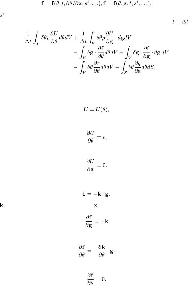
UMATHT
where are state variables.
The Jacobian for Newton’s method is given by (after dropping the subscripts
on U)
The thermal constitutive behavior for this example is now defined. We assume a constant specific
heat for the materia l. The heat conduction in the material is assumed to be governed by Fourier’s law.
The internal thermal energy per unit mass is defined as
with
where c is the specific heat of the material and
Fourier’s law for heat conduction is give n as
where is the thermal conductivity matrix and is position, so that
and
The assumption of conductivity without any temperature dependence implies that
1.1.37–7
Abaqus ID:
Printed on:
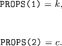
UMATHT
No state variables are needed for this m aterial, so the allocation of space for them is not necessary.
A thermal user material definition can be used to read in the two constants for our simple case,
namely the specific heat, c, and the coefficient of thermal conduc tivity, k,sothat
SUBROUTINE UMATHT(U,DUDT,DUDG,FLUX,DFDT,DFDG,
1 STATEV,TEMP,DTEMP,DTEMDX,TIME,DTIME,PREDEF,DPRED,
2 CMNAME,NTGRD,NSTATV,PROPS,NPROPS,COORDS,PNEWDT,
3 NOEL,NPT,LAYER,KSPT,KSTEP,KINC)
C
INCLUDE 'ABA_PARAM.INC'
C
CHARACTER*80 CMNAME
DIMENSION DUDG(NTGRD),FLUX(NTGRD),DFDT(NTGRD),
1 DFDG(NTGRD,NTGRD),STATEV(NSTATV),DTEMDX(NTGRD),
2 TIME(2),PREDEF(1),DPRED(1),PROPS(NPROPS),COORDS(3)
C
COND = PROPS(1)
SPECHT = PROPS(2)
C
DUDT = SPECHT
DU = DUDT*DTEMP
U = U+DU
C
DO I=1, NTGRD
FLUX(I) = −COND*DTEMDX(I)
DFDG(I,I) = −COND
END DO
C
RETURN
END
1.1.37–8
Abaqus ID:
Printed on:

UMESHMOTION
1.1.38 UMESHMOTION: User subroutine to specify mesh motion constraints during
adaptive meshing.
Product:
Abaqus/Standard
References
•
“Defining ALE adaptive m esh domains in Abaqus/Standard,” Section 12.2.6 of the Abaqus Analysis
User’s Manual
• *
ADAPTIVE MESH
• *
ADAPTIVE MESH CONSTRAINT
Overview
User subroutine UMESHMOTION:
•
can be used to define the motion of nodes in an adaptiv e mesh constraint node set ; and
•
can call utility routines GETVRN, GETNODETOELEMCONN,andGETVRMAVGATNODE to access
results data at the node.
Accessing node point data
You are provided with access to the values of the node point quantities at the end of the increment
through the utility routine GETVRN described in “Obta ining node point informa tion,” Section 2. 1.9.
You can also access values of material point quantities extrapolated to, and averaged, at nodes at the
end of the increment through the utility routine GETVRMAVGATNODE described in “Obtaining material
point information averaged at a node,” Section 2.1.8. GETVRMAVGATNODE requires the list of elements
attached to the node , which is obtained by calling the utility routine GETNODETOELEMCONN described
in “Obtaining node to element connectivity,” Section 2.1.10.
User subroutine interface
SUBROUTINE UMESHMOTION(UREF,ULOCAL,NODE,NNDOF,
* LNODETYPE,ALOCAL,NDIM,TIME,DTIME,PNEWDT,
* KSTEP,KINC,KMESHSWEEP,JMATYP,JGVBLOCK,LSMOOTH)
C
INCLUDE 'ABA_PARAM.INC'
C
DIMENSION ULOCAL(NDIM),JELEMLIST(*)
DIMENSION ALOCAL(NDIM,*),TIME(2)
DIMENSION JMATYP(*),JGVBLOCK(*)
C
1.1.38–1
Abaqus ID:
Printed on:

UMESHMOTION
user coding to define ULOCAL
and, optionally PNEWDT
RETURN
END
Variable to be defined
ULOCAL
Components of the m esh displacement or velocity of the adaptive mesh constraint node, described in
the coordinate system ALOCAL. ULOCAL will be pas sed into the routine as value s determined by the
mesh sm oothing algorithm. All components of the mesh displacement or velocity will be applied; i.e.,
you do not have the ability to select the directions in which the mesh displacement should be applied.
Variables that can be updated
PNEWDT
Ratio of s uggested new time inc rement to the tim e increment currently being used (DTIME,see
below). This variable allows you to provide input to the automatic t ime incrementation algorithms in
Abaqus/Standard (if automatic time incrementation is chosen).
PNEWDT is set to a large value before each call to UMESHMOTION.
The suggested new time increment provided to the automatic time integration algorithms is
PNEWDT × DTIME,wherethePNEWDT used i s the minimum value for all calls to user subroutines
that allow redefinition of PNEWDT for this increment.
If automatic time incrementation is not selected in the analysis procedure, values of PNEWDT
greater than 1.0 will be ignored and values of PNEWDT les s than 1.0 will cause the job to te rminate.
LSMOOTH
Flag specifying that surface smoothing be applied after application of the mesh motion constraint. Set
LSMOOTH to 1 to enable surface smoothing. When this flag is se t, the constraint defined in ULOCAL
will be modified by the smoothing algorithm. In cases where ULOCAL describes mesh mot ion normal
to a surface, the smoothing will have a minor im pact on this normal component of mesh m otion.
Variables passed in for information
UREF
The value of the user-specified displacement or velocity provided as part of the adaptive mesh constraint
definition. This value is updated based on any amplitude definitions used with the adaptive mesh
constraint or default ramp a mplitude variations associated with the current step.
1.1.38–2
Abaqus ID:
Printed on:
UMESHMOTION
NODE
Node number.
NNDOF
Number of degrees of freedom at the node.
LNODETYPE
Node type flag.
LNODETYPE=1 indicates that the node is on the interior of the adaptive mesh region.
LNODETYPE=2 indicates that the node is involved in a tied constraint.
LNODETYPE=3 indicates that the node is at the corner of the boundary of an adaptive mesh region.
LNODETYPE=4 indicates that the node lies on the edge of a boundary of an adaptive m esh region.
LNODETYPE=5 indicates that the node lies on a flat surface on a boundary of the adaptive mesh
region.
LNODETYPE=6 indicates that the node participates in a constraint (other than a tied constraint)
as a master node.
LNODETYPE=7 indicates that the node participates in a constraint (other than a tied constraint)
as a slave node.
LNODETYPE=10 indicates that a concentrated load is applied to the node.
ALOCAL
Local coordinate system aligned with the tangent to the adaptive m esh dom ain at the node. If the node
is on the interior of the adaptive mesh domain, ALOCAL will be set to the identity matrix. In other
cases the 1-direction is along an edge or in the plane of a flat surface. When NDIM=2, the 2-direction
is normal to the surface. When NDIM=3, the 2-direction also lies in the plane of a flat surface or is
arbitrary if the node is on an edge. When NDIM=3 the 3-direction is normal to the surface or is arbitrary
if the node is on an edge.
NDIM
Number of coordinate dimensions.
TIME(1)
Current value of step time.
TIME(2)
Current value of total time.
DTIME
Time increm ent.
KSTEP
Step number.
KINC
Increment number.
1.1.38–3
Abaqus ID:
Printed on:
UMESHMOTION
KMESHSWEEP
Mesh sweep number.
JMATYP
Variable that must be passed into the GETVRMAVGATNODE utility routine to access local results at the
node.
JGVBLOCK
Variable that must be passed into the GETVRN, GETNODETOELEMCONN,andGETVRMAVGATNODE
utility routines to access local results at the node.
1.1.38–4
Abaqus ID:
Printed on:

UMOTION
1.1.39 UMOTION: User subroutine to specify motions during cavity radiation heat transfer
analysis or steady-state transport analysis.
Product:
Abaqus/Standard
References
•
“Cavity radiation,” Section 37.1.1 of the Abaqus Analysis User’s Manual
•
“Steady-state transport analysis ,” Section 6.4.1 of the Abaqus Analysis User’s Manual
• *
MOTION
• *
TRANSPORT VELOCITY
Overview
User subroutine UMOTION:
•
can be used eithe r to defin e the magnit ude o f the translational motion for degre es o f freedom
specified as a predefined field in a cavity radiation heat transfer analysis or to define the magnitude
of the rotational velocity in a steady-state transport step; and
•
will overwrite any motion or transport velocity magnitudes if they are defined directly (and possibly
modified by including an amplitud e reference) outside the user subroutine.
User subroutine interface
SUBROUTINE UMOTION(U,KSTEP,KINC,TIME,NODE,JDOF)
C
INCLUDE 'ABA_PARAM.INC'
C
DIMENSION U,TIME(2)
C
user coding to define U
RETURN
END
1.1.39–1
Abaqus ID:
Printed on:

UMOTION
Variable to be defined
U
Total value of the component of the translation due to prescribed mot ion for the degree of freedom
specified by JDOF. U will be passed into the routine as the value defined by any magnitude and/or
amplitude specification in the motion definition for the degree of freedom JDOF. The total value of
the translation must be given in user subroutine UMOTION, regardless of the type of motion defined
(displacement or velocity).
When used in conjunction with a steady-state transport analysis, U define s the magnitude of the
rotational velocity. In such a case JDOF is passed in as 0.
Variables passed in for information
KSTEP
Step number.
KINC
Increment number.
TIME(1)
Current value of step time.
TIME(2)
Current value of total time.
NODE
Node number.
JDOF
Degree of freedom. When used in a steady-state transport analysis, JDOF is passed in as 0.
1.1.39–2
Abaqus ID:
Printed on:

UMULLINS
1.1.40 UMULLINS: User subroutine to define damage variable for the Mullins effect
material model.
Product:
Abaqus/Standard
References
•
“Mullins effect in rubberlike m aterials,” Section 19.6.1 of the Abaqus Analysis User’s Manual
• *
MULLINS EFFECT
•
“Mullins effect and permanent set,” Section 2.2.3 of the Abaqus Verification Manual
Overview
User subroutine UMULLINS:
•
can be used to define the damage varia ble for the Mullins effect material model, incl uding the use
of the Mullins effect approach to model energy dissipation in elastomeric foams;
•
will be called at all material calculation points of elements for which the material definition co n tains
a user-defined Mullins effect; and
•
should be used when you do not want to use the form of the damage variable, ,thatisusedby
Abaqus/Standard.
User subroutine interface
SUBROUTINE UMULLINS(NUMPROPS,PROPS,UMAXNEW,UMAXOLD,SEDDEV,
1 ETA,DETADW,DMGDISSOLD,DMGDISSNEW,SENERNEW,NUMSTATEV,STATEV,
2 TEMP,DTEMP,NUMFIELDV,FIELDV,FIELDVINC,CMNAME,LINPER)
C
INCLUDE 'ABA_PARAM.INC'
C
CHARACTER*80 CMNAME
DIMENSION PROPS(*),STATEV(*),FIELDV(*),FIELDVINC(*)
user coding to define ETA, DETADW,
and, optionally, DMGDISSNEW, SENERNEW, STATEV
RETURN
END
1.1.40–1
Abaqus ID:
Printed on:

UMULLINS
Variables to be defined
ETA
The damage variable,
.
DETADW
The derivative of the damage variable with respect to the elastic strain energy density of the undama ged
material,
. This quantity is needed for the Jacobian of the ove rall system of equations and needs to
be defined accurately to ensure good convergence characteristics.
Variables that can be updated
DMGDISSNEW
The energy dissipation density at the end of the incre ment. This quant ity can be defined either i n total
form or in an incrementa l manner using the old value of the damage dissipation DMGDISSOLD and the
increment in damage dissipation. This quantity is used for output purpose s only.
SENERNEW
The recovera ble strain energy density at the e nd of the increment. This quantity is used for output
purposes only.
STATEV
Array containing the user-defined solution-dependent state variables at this point. These are supplied a s
values at the start of the increment or as values updated by other user subroutines (see “User subroutines:
overview,” Section 15.1.1 of the Abaqus Analysis User’s Manual) and must be returned as values at
the end of the increment.
Variables passed in for information
UMAXNEW
The value, at the end of the increment, of the maximum primary strain energy density over its entire
deformation history.
UMAXOLD
The value, at the beginning of the increment, of the m aximum primary strain energy density over its
entire deformation history.
SEDDEV
The value, at the end of the increm ent, of the deviatoric primary strain energy density when the primary
material behavior is hyperelastic. The va lue, at the end of the increment, of the total primary strain
energy density when the primary material behavior is hyperfoam.
DMGDISSOLD
The value of energy dissipated at the beginning of the increment.
1.1.40–2
Abaqus ID:
Printed on:
UMULLINS
CMNAME
User-specified material name, left justified.
NUMSTATEV
Number of solution-dependent state variables associated with this material (defined as described in
“Allocating space” in “U ser subroutines: overview,” Section 15.1.1 of the A baqus Analysis User’s
Manual).
NUMPROPS
Number of material properties entered for this user-defined hyperelastic m aterial.
PROPS
Array of material properties entered for this user-defined hyperelastic m aterial.
TEMP
Tem perature at the start of the increment.
DTEMP
Increment of temperature.
NUMFIELDV
Number of field variables.
FIELDV
Array of interpolated values of predefined field variables at this m aterial point at the beginning of the
increment based on the values read in at the nodes (initial values at the beginning of the analysis and
current values during the analysis).
FIELDVINC
Array of increments of predefined field variables at this material point for this increment; this includes
any values updated by user subroutine USDFLD.
LINPER
Linear perturbation flag. LINPER=1 if the s tep is a linear perturbation step. LINPER=0 if the step is
a general step.
1.1.40–3
Abaqus ID:
Printed on:

UPOREP
1.1.41 UPOREP: User subroutine to define initial fluid pore pressure.
Product:
Abaqus/Standard
References
•
“Initial conditions in Abaqus/Standard and Abaqus/Explicit,” Section 30.2.1 of the Abaqus Analysis
User’s Manual
•
“Coupled pore fluid diffusion and stress analysis,” Section 6.8.1 of the Abaqus Analysis User’s
Manual
• *
INITIAL CONDITIONS
Overview
User subroutine UPOREP:
•
allows for the specification of the i nitial pore pressure values of a porous medium;
•
can be used to de fine initial pore pressure values as functions of nodal coordinates and/o r node
numbers; and
•
will be called to define initial fluid pore pressure values at all nodes of a coupled pore fluid diffusion
and stress analysis whenever user-defined initial pore pressure conditions are specified.
User subroutine interface
SUBROUTINE UPOREP(UW0,COORDS,NODE)
C
INCLUDE 'ABA_PARAM.INC'
C
DIMENSION COORDS(3)
C
user coding to define UW0
RETURN
END
Variable to be defined
UW0
Initial fluid pore pressure.
1.1.41–1
Abaqus ID:
Printed on:

UPOREP
Variables passed in for information
COORDS
An array containing the current coordinates of this node.
NODE
Node number.
1.1.41–2
Abaqus ID:
Printed on:

UPRESS
1.1.42 UPRESS: User subroutine to specify prescribed equivalent pressure stress
conditions.
Product:
Abaqus/Standard
References
•
“Mass diffusion analysis,” Section 6.9.1 of the Abaqus Analysis User’s Manual
• *
PRESSURE STRESS
•
“UTEMP, UFIELD, UMASFL,andUPRESS,” Section 4.1.25 of the Abaqus Verification Manual
Overview
User subroutine UPRESS:
•
allows you to prescribe equivalent pressure stress values at the nodes of a model;
•
will be called in a m ass diffusion analysis whenever a current value of equivalent pressure stress is
needed for a node that has user-defined pressure stress conditions;
•
can be used to modify any pressure stresses read in from a results file; and
•
ignores any equivalent pressure stresses provided for the associated pressure stress definition outside
the user subroutine.
User subroutine interface
SUBROUTINE UPRESS(PRESS,KSTEP,KINC,TIME,NODE,COORDS)
C
INCLUDE 'ABA_PARAM.INC'
C
DIMENSION TIME(2), COORDS(3)
C
user coding to define PRESS
RETURN
END
Variable to be defined
PRESS
Total value of th e equivalent pressure stress at the node.
1.1.42–1
Abaqus ID:
Printed on:

UPRESS
You m ay have also requested equivalent pressure stress to be set in one of two other ways: from
a previously generated results file or via direct data input. When PRESS is passed into user subroutine
UPRESS, it will contain equivalent pressure stresses obtained from the results file only. You can modify
these values within this routine. Any values given as direct data input will be ignored.
Variables passed in for information
KSTEP
Step number.
KINC
Increment number.
TIME(1)
Current value of step time.
TIME(2)
Current value of total time.
NODE
Node number.
COORDS
An array containing the coordinates of this n ode.
1.1.42–2
Abaqus ID:
Printed on:

UPSD
1.1.43 UPSD: User subroutine to define the frequency dependence for random response
loading.
Product:
Abaqus/Standard
References
•
“Random response analysis,” Section 6.3.11 of the Abaqus Analysis User’s Manual
• *
RANDOM RESPONSE
• *
PSD-DEFINITION
•
“Random response to jet noise e xcitation,” Section 1.4.10 of th e Abaqus Benchmarks Manua l
Overview
User subroutine UPSD:
•
will be called once for each frequency at which calculations w ill be made during a random response
analysis if the frequency function is defined in a user subroutine;
•
is used to define complicated frequency dependencies for the cross-spectral density matrix of the
random loading; and
•
ignores any data given for the associated frequency function outside the user subroutine.
User subroutine interface
SUBROUTINE UPSD(PSD,PSDR,PSDI,FREQ,KSTEP)
C
INCLUDE 'ABA_PARAM.INC'
C
CHARACTER*80 PSD
user coding to define PSDR and PSDI
RETURN
END
Variables to be defined
PSDR
Real part of the frequency function at this frequency.
1.1.43–1
Abaqus ID:
Printed on:

UPSD
PSDI
Imaginary part of the frequency function at this frequency.
Variables passed in for information
PSD
User-specified nam e for this frequency function definition, left justified.
FREQ
Frequency, in radians per time.
KSTEP
Step number.
1.1.43–2
Abaqus ID:
Printed on:

URDFIL
1.1.44 URDFIL: User subroutine to read the results file.
Product:
Abaqus/Standard
References
•
“Results file output format,” Section 5.1.2 of the Abaqus Analysis User’s Manual
•
“Accessing the results file information,” Section 5.1.3 of the Abaqus Analysis User’s Manual
•
“Utility routines for accessing the results file,” Section 5.1.4 of the Abaqus Analysis User’s Manual
Overview
User subroutine URDFIL:
•
can be used to access the results file during an analysis;
•
is called at the end of any increment in which new information is written to the results file;
•
must call the utility routine DBFILE to read records from the results file (see “Utility routines for
accessing the results file,” Section 5.1.4 of the Abaqus Analysis User’s Manual);
•
can call the utility routine POSFIL to read from the resul ts file starting at a specified step and
increment as opposed to the beginning of the file, which wou ld otherwise be done (see “Utility
routines for accessing the results file,” Section 5.1.4 of the Abaqus Analysis User’s Manual);
•
can force an analysis to terminate upon completion of a call by means of the variable LSTOP;
•
allows the last increm ent written to the results file to be overwritten by means of the variable
LOVRWRT;and
•
allows access to the complete results file in a restarted job if the new results file is being appended
to the old results file (see the description of the execution option fil in “Abaqus/Standard,
Abaqus/Explicit, and Abaqus/CFD execution,” Section 3.2.2 of the Abaqus Analysis User ’s
Manual).
User subroutine interface
SUBROUTINE URDFIL(LSTOP,LOVRWRT,KSTEP,KINC,DTIME,TIME)
C
INCLUDE 'ABA_PARAM.INC'
C
DIMENSION ARRAY(513),JRRAY(NPRECD,513),TIME(2)
EQUIVALENCE (ARRAY(1),JRRAY(1,1))
user coding to read the results file
RETURN
1.1.44–1
Abaqus ID:
Printed on:

URDFIL
END
Variables to be defined
In all cases
LSTOP
Flag to indicate whether an analysis should continue. The analysis will be terminated if LSTOP is set
to 1. Otherwise, the analysis will con tinue.
LOVRWRT
Flag to indicate that the information writte n to the results file for the inc rement can be overwritten. If
LOVRWRT is set to 1, information for the current increment will be overwritten by information written
to the results file in a subsequent increment unless the current increment is the final increment written to
the results file. The purpose of this flag is to reduce th e size of the results file by allowing information
for an increment to be overwritten by info rmation for a subsequent increment.
DTIME
Time increment. This variable allows you to provide input to the automatic time incrementation
algorithms in Abaqus (if automatic time incrementation is chosen). It is passed in as the value of
the next time increment to be t aken and can be updated to increase or red uce the time increment. If
automatic tim e incrementation is not selected in the analysis procedure, updated values of DTIME are
ignored.
Only if utility routine POSFIL is called
NSTEP
Desired step at which file reading will begin via utility routine DBFILE.IfNSTEP is se t to 0, the first
available step will be read.
NINC
Desired increment at which file reading will begin via utility routine DBFILE.IfNINC is set to 0, the
first available increment of the specified step w ill be read.
Variables passed in for information
KSTEP
Step number.
KINC
Increment number.
TIME(1)
Value of the step time at the end of the increment.
1.1.44–2
Abaqus ID:
Printed on:

URDFIL
TIME(2)
Value of the total time at the end of the increment.
Example: Terminating an analysis upon exceeding a Mises stress limit
The example below reads the values of Mises stress for the current increment from record 12 in the results
file and term inates the analysis if any of the values of Mises stress written to the results file exceed 2.09
×10
8
. Here, POSFIL is used to position you to read from the current increment.
SUBROUTINE URDFIL(LSTOP,LOVRWRT,KSTEP,KINC,DTIME,TIME)
C
INCLUDE 'ABA_PARAM.INC'
C
DIMENSION ARRAY(513),JRRAY(NPRECD,513),TIME(2)
EQUIVALENCE (ARRAY(1),JRRAY(1,1))
PARAMETER(TOL=2.09D8)
C
C FIND CURRENT INCREMENT.
C
CALL POSFIL(KSTEP,KINC,ARRAY,JRCD)
DO K1=1,999999
CALL DBFILE(0,ARRAY,JRCD)
IF (JRCD .NE. 0) GO TO 110
KEY=JRRAY(1,2)
C
C RECORD 12 CONTAINS VALUES FOR SINV
C
IF (KEY.EQ.12) THEN
IF (ARRAY(3).GT.TOL) THEN
LSTOP=1
GO TO 110
END IF
END IF
END DO
110 CONTINUE
C
RETURN
END
Example: Terminating an analysis when the maximum Mises stress value stops increasing
This example demonstrates the use of URDFIL and POSFIL to stop an analysis when the maximum
value of Mises stress in the model does not increase from one increment in the results file to the next.
1.1.44–3
Abaqus ID:
Printed on:
URDFIL
A data statement is used to save the maximum Mises stress value from the last increment. LOVRWRT is
also used in this case to overwrite an increment in the results file once it has been read in URDFIL.
The subroutine shown below must be modified to define the maximum Mises stress in the data
statement each time a job is restarted. This can be avoided by removing the LOVRWRT=1 statement
and recoding the routine to read both the previous and the current increment to check that the Mises
stress increases from one increment to the next (in this case you must correctly handle the first increment
written to the results file as there will be no previous increment). The results file must also be properly
appended on restart if you wish to compare the values of Mises stress between the first increm ent of a
restart and the final increment of the job being re started. This app roach has the disadvantage that the
results file may become quite large, as n o information in the file will be overwritten.
SUBROUTINE URDFIL(LSTOP,LOVRWRT,KSTEP,KINC,DTIME,TIME)
C
INCLUDE 'ABA_PARAM.INC'
C
DIMENSION ARRAY(513),JRRAY(NPRECD,513),TIME(2)
EQUIVALENCE (ARRAY(1),JRRAY(1,1))
C
C INITIALIZE THE OLD MAXIMUM. FOR A JOB THAT IS BEING RESTARTED
C THIS VALUE SHOULD BE SET TO THE MAXIMUM MISES STRESS IN THE
C ORIGINAL ANALYSIS.
C
DATA OLDMAX/-1.D0/
C
CURRMAX = 0.D0
C
C FIND CURRENT INCREMENT.
C
CALL POSFIL(KSTEP,KINC,ARRAY,JRCD)
C
C SEARCH FOR THE HIGHEST VALUE OF MISES STRESS
C AND STORE THIS IN CURRMAX
C
DO K1=1,999999
CALL DBFILE(0,ARRAY,JRCD)
IF (JRCD.NE.0) GO TO 110
KEY=JRRAY(1,2)
IF (KEY.EQ.12) THEN
IF (ARRAY(3).GT.CURRMAX) CURRMAX=ARRAY(3)
END IF
END DO
110 CONTINUE
C
1.1.44–4
Abaqus ID:
Printed on:
URDFIL
C COMPLETED READING OF CURRENT INCREMENT. NOW CHECK TO
C SEE IF VALUE OF MISES STRESS HAS INCREASED SINCE
C LAST INCREMENT
C
IF (CURRMAX.LE.OLDMAX) LSTOP=1
OLDMAX=CURRMAX
LOVRWRT=1
C
RETURN
END
1.1.44–5
Abaqus ID:
Printed on:

USDFLD
1.1.45 USDFLD: User subroutine to redefine field variables at a material point.
Product:
Abaqus/Standard
References
•
“Obtaining material point information in an Abaqus/Standard analysis,” Section 2.1.6
•
“Material data definition,” Section 18.1.2 of the Abaqus Analysis User’s Manual
• *
USER DEFINED FIELD
•
“Damage and failure of a lam inated com posite plate,” Section 1.1.14 of the Abaqus Example
Problems Manual
•
“USDFLD,” Section 4.1.24 of the A baqus Verification Manual
Overview
User subroutine USDFLD:
•
allows you to define field variables at a material point as functions of time or of any of the available
material point quantities listed in the Output Variable Identifiers table (“Abaqus/Standard output
variable identifiers,” Section 4.2.1 of the Abaqus Analysis User’s Manual) except the user-defined
output variables UVARM and UVARMn;
•
can be used to introduce solution-dependent material properties since such properties can easily be
defined as functions of field variables;
•
will be called at all material points of elements for which the m aterial definition includes user-
defined field variables;
•
must call utility routine GETVRM to access material point data;
•
can use and update state variables; and
•
can be used in conjunction with user subroutine UFIELD to prescribe predefined field variables.
Explicit solution dependence
Since this routine provides access to material point quantities only at the start of the increment, the
solution dependence introduced in this way is explicit: the material properties for a given increment are
not influenced by the results obtained during the increment. Hence, the accuracy of the results depends
on the size of the time increment. Therefore, you can control the time increment in this routine by m eans
of the variable PNEWDT.
Defining field variables
Before user subroutine USDFLD is called, the values of the fi eld variab les at the material point are
calculated by interpolation from the values defined at the nodes. Any changes to the field variables
in the user subroutine are local to the material point: the nodal field variables retain the values defined
1.1.45–1
Abaqus ID:
Printed on:

USDFLD
as initial conditions, predefined field variables, or in user subroutin e UFIELD. The values of the field
variables defined in this routine are used to calculate values of m aterial properties that are defined to
depend on field variables and are passed into other user subroutines that are called at the material point,
such as the following:
•
CREEP
•
HETVAL
•
UEXPAN
•
UHARD
•
UHYPEL
•
UMAT
•
UMATHT
•
UTRS
Output of the user-defined field variables at the material points can be obtained with the element
integration point output variable FV (see “Abaqus/Standard output variable identifiers,” Section 4.2.1
of the Abaqus Analysis User’s Manua l).
Accessing material point data
You are provided with access to the values of the material point quantities at the start of the increment (or
in the base state in a linear perturbation step) through the utility routine GETVRM described in “Obtaining
material point information in an Abaqus/ Standard analysis,” Section 2.1.6. The values of the ma terial
point quantities are obtained by calling GETVRM with the appropriate output variable keys. The values
of the material point data are recovered in the arrays ARRAY, JARRAY,andFLGRAY for floating point,
integer, and character data, respectively. You may not get values of some material point quantities that
have not been defined at the start of the increment; e.g., ER.
State variables
Since the redefinition of field va riables in USDFLD is local to the current increment (field variables are
restored to the values interpolated from the nodal values at the start of each increment), any history
dependence required to update material propertie s by using this subroutine must be introduced with user-
defined state variables.
The state variables can be updated in USDFLD and then passed into other user subroutines that can
be called at this material point, such a s those listed above. You specify the number of such state variables,
as shown in the exam ple at the end of this section (see also “Allocating space” in “User subroutines:
overview,” Section 15.1.1 of the Abaqus Analysis User’s Manual).
User subroutine interface
SUBROUTINE USDFLD(FIELD,STATEV,PNEWDT,DIRECT,T,CELENT,
1 TIME,DTIME,CMNAME,ORNAME,NFIELD,NSTATV,NOEL,NPT,LAYER,
1.1.45–2
Abaqus ID:
Printed on:

USDFLD
2 KSPT,KSTEP,KINC,NDI,NSHR,COORD,JMAC,JMATYP,MATLAYO,LACCFLA)
C
INCLUDE 'ABA_PARAM.INC'
C
CHARACTER*80 CMNAME,ORNAME
CHARACTER*3 FLGRAY(15)
DIMENSION FIELD(NFIELD),STATEV(NSTATV),DIRECT(3,3),
1 T(3,3),TIME(2)
DIMENSION ARRAY(15),JARRAY(15),JMAC(*),JMATYP(*),COORD(*)
user coding to define FIELD and, if neces sary, STATEV and PNEWDT
RETURN
END
Variable to be defined
FIELD(NFIELD)
An array containing the field variables at the current material point. These are passed in with the values
interpolated from the nodes at the end of the current increment, as specified with initial condition
definitions, predefined field variable definitions, or user subroutine UFIELD. The interpolation is
performed using the same scheme used to interpolate temperatures: an average value is used for linear
elements; an approximate linear variation is used for quadratic elements (also see “Solid (continuum)
elements,” Section 25.1.1 of the Abaqus Analysis User’s Manual). The updated values are used to
calculate the values of material properties that are defined to depend on field variables and are passed
into other user subroutines (CREEP, HETVAL, UEXPAN, UHYPEL, UMAT, UMATHT,andUTRS)that
are called at this m aterial point.
Variables that can be updated
STATEV(NSTATV)
An array containing the solution-dependent state variables. These are passed in as the values at the
beginning of the increment. In all cases STATEV can be upda ted in this subroutine, and the updated
values are passed into other user subroutines (CREEP, HETVAL, UEXPAN, UMAT, UMATHT,andUTRS)
that are called at this material point. The number of state variables associated with this material point
is defined as described in “Allocating space” in “User subroutines: overview,” Section 15.1.1 of the
Abaqus Analysis User’s Manual.
PNEWDT
Ratio of suggested new time increment to the time increment being used (DTIME, see below).
This variable allows you to provide input to the automatic time incrementation algorithms in
Abaqus/Standard (if automatic time incrementation is chosen).
1.1.45–3
Abaqus ID:
Printed on:

USDFLD
PNEWDT is set to a large value before each call to USDFLD.
If PNEWDT is redefined to be less than 1.0, Abaqus/Standard must abandon the time increment
and attem pt it again with a smaller time increment. The suggested new time increment provided to the
automatic time integration algorithms is PNEWDT × DTIME, wher e the PNEWDT used is the minimum
value for all calls to user subroutines that allow redefinition of PNEWDT for this iteration.
If PNEWDT is given a v alue that is greater than 1.0 for all calls to user subroutines for this iteration
and the increment converges in this iteration, A baqus/Standard m ay increase the time increment. The
suggested new time increment provided to the automatic time integration algorithms is PNEWDT ×
DTIME, where the PNEWDT used is the minimum value for all calls to user subroutines for this iteration.
If automatic time incrementation is not selected in the anal ysis proc edure, values of PNEWDT that
are greater than 1.0 will be ignored and values of PNEWDT that are less than 1.0 will cause the job to
terminate.
Variables passed in for information
DIRECT(3,3)
An array containing the direction cosines of the material directions in terms of the global b
asis
directions. DIRECT(1,1), DIRECT(2,1), DIRECT(3,1) give the (1, 2, 3) components of the
first material direction; DIRECT(1,2), DIRECT(2,2), DIRECT(3,2) give the second m aterial
direction, etc. For shell and m embrane elem ents, the first two directions are in the plane of the elem ent
and the third direction is the normal. This information is not available for beam element s.
T(3,3)
An array containing the direction cosines of the material orientation com ponents relative to the element
basis directions. This is the orientation that d efines the materia l d irections (DIRECT)intermsof
the element basis directions. For continuum elements T and DIRECT are identical. For shell and
mem brane elements T(1,1)
, T(1,2) , T(2,1) , T(2,2) ,
T(3,3)
, and all other components are zero, where is the counterclockwise rotation around the
normal vector that defines the orie ntation. If no orientation is used, T is an identity matrix. Orientation
is not available for beam elements.
CELENT
Characteristic elem ent length. This is a typical length of a line across an element for a first-order
element; it is half of the sam e typical length for a second-order element. For beams and trusses it is a
characteristic length along the element axis. For membranes and shells it is a characteristic length in
the reference surface. For axisymm etric elements it is a characteristic length in the
plane only.
TIME(1)
Value of step time at the beginning of the current increment.
TIME(2)
Value of total tim e at the beginning of the current increment.
1.1.45–4
Abaqus ID:
Printed on:
USDFLD
DTIME
Time increm ent.
CMNAME
User-specified material name, left justified.
ORNAME
User-specified local orientation name, left justified.
NFIELD
Number of field variables defined at this m aterial point.
NOEL
Element number.
NPT
Integration point number.
LAYER
Layer number (for composite shells and layered solids).
KSPT
Section point number within the current layer.
KSTEP
Step number.
KINC
Increment number.
NDI
Number of direct stress components at this point.
NSHR
Number of shear stress com ponents at this point.
COORD
Coordinates at this material point.
JMAC
Variable that must be passed into the GETVRM utility routine to access an output variable using the
utility routine.
JMATYP
Variable that must be passed into the GETVRM utility routine to access an output variable using the
utility routine.
1.1.45–5
Abaqus ID:
Printed on:

USDFLD
MATLAYO
Variable that must be passed into the GETVRM utility routine to access an output variable using the
utility routine.
LACCFLA
Variable that must be passed into the GETVRM utility routine to access an output variable using the
utility routine.
Example: Damaged elasticity model
Included below is an example of user subroutine USDFLD. In this example a truss element is loaded
in tension. A dam aged elasticity model is introduced: the modulus decreases as a function of the
maximum tensile strain that occurred during the loading history. The maximum tensile strain is store d
as a solution-dependent state variable—see “Defining solution-dependent field variables” in “Predefined
fields,” Section 30.6.1 of the Abaqus Analysis User’s Manual.
Input file
*
HEADING
DAMAGED ELASTICITY MODEL WITH USER SUBROUTINE USDFLD
*
ELEMENT, TYPE=T2D2, ELSET=ONE
1, 1, 2
*
NODE
1, 0., 0.
2, 10., 0.
*
SOLID SECTION, ELSET=ONE, MATERIAL=ELASTIC
1.
*
MATERIAL, NAME=ELASTIC
*
ELASTIC, DEPENDENCIES=1
** Table of modulus values decreasing as a function
** of field variable 1.
2000., 0.3, 0., 0.00
1500., 0.3, 0., 0.01
1200., 0.3, 0., 0.02
1000., 0.3, 0., 0.04
*
USER DEFINED FIELD
*
DEPVAR
1
*
BOUNDARY
1, 1, 2
2, 2
*
STEP
*
STATIC
0.1, 1.0, 0.0, 0.1
1.1.45–6
Abaqus ID:
Printed on:
USDFLD
*
CLOAD
2, 1, 20.
*
END STEP
*
STEP
*
STATIC
0.1, 1.0, 0.0, 0.1
*
CLOAD
2, 1, 0.
*
END STEP
*
STEP, INC=20
*
STATIC
0.1, 2.0, 0.0, 0.1
*
CLOAD
2, 1, 40.
*
END STEP
User subroutine
SUBROUTINE USDFLD(FIELD,STATEV,PNEWDT,DIRECT,T,CELENT,
1 TIME,DTIME,CMNAME,ORNAME,NFIELD,NSTATV,NOEL,NPT,LAYER,
2 KSPT,KSTEP,KINC,NDI,NSHR,COORD,JMAC,JMATYP,MATLAYO,
3 LACCFLA)
C
INCLUDE 'ABA_PARAM.INC'
C
CHARACTER*80 CMNAME,ORNAME
CHARACTER*3 FLGRAY(15)
DIMENSION FIELD(NFIELD),STATEV(NSTATV),DIRECT(3,3),
1 T(3,3),TIME(2)
DIMENSION ARRAY(15),JARRAY(15),JMAC(*),JMATYP(*),
1 COORD(*)
C
C Absolute value of current strain:
CALL GETVRM('E',ARRAY,JARRAY,FLGRAY,JRCD,JMAC,JMATYP,
MATLAYO,LACCFLA)
EPS = ABS( ARRAY(1) )
C Maximum value of strain up to this point in time:
CALL GETVRM('SDV',ARRAY,JARRAY,FLGRAY,JRCD,JMAC,JMATYP,
MATLAYO,LACCFLA)
EPSMAX = ARRAY(1)
C Use the maximum strain as a field variable
FIELD(1) = MAX( EPS , EPSMAX )
C Store the maximum strain as a solution dependent state
1.1.45–7
Abaqus ID:
Printed on:
USDFLD
C variable
STATEV(1) = FIELD(1)
C If error, write comment to .DAT file:
IF(JRCD.NE.0)THEN
WRITE(6,*) 'REQUEST ERROR IN USDFLD FOR ELEMENT NUMBER ',
1 NOEL,'INTEGRATION POINT NUMBER ',NPT
ENDIF
C
RETURN
END
1.1.45–8
Abaqus ID:
Printed on:

UTEMP
1.1.46 UTEMP: User subroutine to specify prescribed temperatures.
Product:
Abaqus/Standard
References
•
“Predefined fields,” Section 30.6.1 of the Abaqus Analysis User’s Manual
• *
TEMPERATURE
•
“LE11: Solid cylinder/taper/sphere—temperature loading,” Section 4.2.11 of the Abaqus
Benchmarks Manual
•
“UTEMP, UFIELD, UMASFL,andUPRESS,” Section 4.1.25 of the Abaqus Verification Manual
Overview
User subroutine UTEMP:
•
allows you to prescribe tem peratures at the nodes of a model;
•
will be called whenever a current value of temperature is needed for a node that is listed under a
user-defined temperature field definition;
•
ignores any temperatures provided for the associated temperature field definition outside the user
subroutine; and
•
can be used to modify any temperatures read in from a results file.
User subroutine interface
SUBROUTINE UTEMP(TEMP,NSECPT,KSTEP,KINC,TIME,NODE,COORDS)
C
INCLUDE 'ABA_PARAM.INC'
C
DIMENSION TEMP(NSECPT), TIME(2), COORDS(3)
C
user coding to define TEMP
RETURN
END
1.1.46–1
Abaqus ID:
Printed on:

UTEMP
Variable to be defined
TEMP(NSECPT)
Array of tempera ture values at node number NODE. If the node is not connected to a beam or she ll
element, only one value of temperature must be returned (NSECPT=1). Otherwise, the number of
temperatures to be returned depends on the mode of temperature and field variable input selected for
the beam or shell section. The following cases are possible:
1. Temperatures and field variables for a beam section are given as values at the points shown in
the beam section descriptions. The number of values required, NSECPT, is determined by the
particular section type specified, as described in “B eam cross-section library,” Section 26.3.9 of
the Abaqus Analysis User’s Manual.
2. Temperatures and field variables are given as values at n equally spaced points through each layer
of a shell section. The number of values required, NSECPT,isequalton.
3. Temperatures and field variables for a beam section are given as values at the origin of the cross-
section together with gradients with respect to the 2-direction and, for three-dimensional beams,
the 1-direction of the section; or temperatures and field variables for a shell section are given as
values at the reference surface together with gradients with respect to the thickness. The number
of values required, NSECPT, is 3 for three-dimensional beams, 2 for two-dimensional beams,
and 2 for shells. Give the midsurface value first, followed by the first and (if necessary) second
gradients, as described in “Beam elem ents,” Section 26.3 of the Abaqus Analysis User’s Manual,
and “Shell elem ents,” Section 26.6 of the Abaqus Analysis User’s Manual.
You can also request temperatures to be set in one of two other ways: from a previously generated
results file or via direct data input. When array TEMP is passed into user subroutine UTEMP,itwill
contain temperatures obtained from the results file only. You can modify these values within this
routine. Any values given as direct data input will be ign ored.
Variables passed in for information
NSECPT
Maximum number of section values required for any node i n the model.
KSTEP
Step number.
KINC
Increment number.
TIME(1)
Current value of step time.
TIME(2)
Current value of total time.
1.1.46–2
Abaqus ID:
Printed on:
UTEMP
NODE
Node number.
COORDS
An array containing the current coordinates of this point. These are the current coordinates if geometric
nonlinearity is accounted for during the step (see “Procedures: overview,” Section 6.1.1 of the Abaqus
Analysis User’s Manual); otherwise, the array contains the original coordinates of the node.
1.1.46–3
Abaqus ID:
Printed on:

UTRACLOAD
1.1.47 UTRACLOAD: User subroutine to specify nonuniform traction loads.
Product:
Abaqus/Standard
References
•
“Distributed loads,” Section 30.4.3 of the Abaqus Analysis User’s Manual
• *
DLOAD
• *
DSLOAD
•
“Distributed traction and edge loads,” Section 1.4.17 of the Abaqus Verification Manual
Overview
User subroutine UTRACLOAD:
•
can be used to define the variation of the distributed traction loa d magnitude as a function of position,
time, element number, load integra tion point number, etc.;
•
if needed, can be used to define the initial loading direction for the distributed traction load as a
function of position, eleme nt number, load integration poi nt number, etc.;
•
will be called at each load integration point for each element-based, edge-based, or surface-based
nonuniform distributed traction load definition during stress analysis;
•
cannot be used in mode-bas ed procedures to describe the time variation of the load; and
•
ignores any amplitude references that may appear w ith the associated step definition or nonuniform
distributed traction load definition.
User subroutine interface
SUBROUTINE UTRACLOAD(ALPHA,T_USER,KSTEP,KINC,TIME,NOEL,NPT,
1 COORDS,DIRCOS,JLTYP,SNAME)
C
INCLUDE 'ABA_PARAM.INC'
C
DIMENSION T_USER(3), TIME(2), COORDS(3), DIRCOS(3,3)
CHARACTER*80 SNAME
user coding to define ALPHA and T_USER
RETURN
END
1.1.47–1
Abaqus ID:
Printed on:

UTRACLOAD
Variables to be defined
ALPHA
Magnitude of the distributed traction load. Units are FL
−2
for surface loads, FL
−1
for edge loads, and F
for edge moments. ALPHA is p assed into the routine as the magnitude of the load s pecified as part of
the elem ent-based or surface-based distributed load definition. If the magnitude is not defined, ALPHA
is passed in as zero. For a static analysis that uses the modified Riks method (“Unstable collapse and
postbuckling analysis,” Section 6.2.4 of the Abaqu s Analysis User’s Manual) ALPHA must be defined
as a function of the load proportiona lity factor,
. The distributed load magnitude is not available for
output purposes.
T_USER
Loading direction of the distributed traction load. T_USER is passed into the routine as the load
direction specified as part of the elem ent-based or surface-based distributed load definition. The
vector T_USER passed out of the subroutine is used as the initial loading direction
discussed in
“Distributed loads,” Section 30.4.3 of the Abaqus Analysis User’s Manual. The direction of T_USER
as defi ned by the subroutine should not change during a step. If it does, co nvergence difficultie s
might arise. Load directions are needed only for a nonuniform general surface traction, shear surface
traction, and general edge traction. If a direction is defined for the nonuniform normal edge traction,
shear edge traction, transverse edge traction, or edge mom ent, it will be ignored. See “Distributed
loads,” Section 30.4.3 of the Abaqus Analysis User ’s Manual, for details.
Variables passed in for information
KSTEP
Step number.
KINC
Increment number.
TIME(1)
Current value of step time or current value of the load proportionality factor,
,inaRiksstep.
TIME(2)
Current value of total time.
NOEL
User-defined elem ent num ber.
NPT
Load integration point number within the element or on the element’s surface, depending on the load
type.
1.1.47–2
Abaqus ID:
Printed on:

UTRACLOAD
COORDS
An array containing the coordinates of the load integration point. These are the current coordinates
if geometric nonlinearity is accounted for during the step (see “Procedures: overview,” Section 6.1.1
of the Abaqus Analysis User’s Manual); otherwise, the array contains the original coordinates of the
point.
DIRCOS
Orientation of the face or edge in the reference configuration. For three-dimensional facets the first and
second colum ns are the normalized local directions in the plane of the surface, and the third column
is the norm al to the face. For solid elements the norm al points inward, which is the negative of what
is defined in “Conventions,” Section 1.2.2 of the Abaqus Analysis User’s Manua l; for shell elements
the normal definition is consistent w ith the convention. For two-dimensional facets the first column
is the normalized tangent, the second column is the facet normal, and the third colum n is not used.
For three-dimensional shell edges the first column is the tangent to the shell edg e (shear direction),
the second column is the in-plane normal (normal direction), and the third column is the normal to the
plane of the shell (transverse direction).
JLTYP
Identifies the load type for w hich this call to UTRACLOAD is being m ade. The load type may be an
element-based surface load, an edge-based load, or a surface-based load. This variable identifies the
element face or edge for which this call to UTRACLOAD is being made. This information is useful
when several different nonuniform distributed loads are being imposed on an element at the same
time. See Part VI, “Elements,” of the Abaqus Analysis User’s Manual for element face and edge
identification. The load labels are shown in Table 1.1.47–1. For surface- or edge-based loading
(TRSHRNU, TRVECNU, EDLDNU, EDNORNU, EDSHRNU, EDTRAN U, EDMOM NU), j in the
load type identifies the face or edge of the elem ent underlying the surface.
Table 1.1.47–1 JLTYP values for surface traction and edge load labels.
Load Label JLTYP Load Label JLTYP Load Label JLTYP
TRSHRNU 510+j EDLDNU 540+j EDTRANU 570+j
TRSHR1NU 511 EDLD1NU 543 EDTRANU 573
TRSHR2NU 512 EDLD2NU 544 EDTRANU 574
TRSHR3NU 513 EDLD3NU 545 EDTRANU 575
TRSHR4NU 514 EDLD4NU 546 EDTRANU 576
TRSHR5NU 515 EDNORNU 550+j EDMOMNU 580+j
TRSHR6NU 516 EDNOR1NU 553 EDMOM1NU 583
TRVECNU 520+j EDNOR2NU 554 EDMOM2NU 584
TRVEC1NU 521 EDNOR3NU 555 EDMOM3NU 585
1.1.47–3
Abaqus ID:
Printed on:

UTRACLOAD
Load Label JLTYP Load Label JLTYP Load Label JLTYP
TRVEC2NU 522 EDNOR4NU 556 EDMOM4NU 586
TRVEC3NU 523 EDSHRNU 560+j
TRVEC4NU 524 EDSHRNU 563
TRVEC5NU 525 EDSHRNU 564
TRVEC6NU 526 EDSHRNU 565
EDSHRNU 566
SNAME
Surface name for a surface-based load definition. For an element-based or edge-based load the surface
name is passed in as blank.
1.1.47–4
Abaqus ID:
Printed on:

UTRS
1.1.48 UTRS: User subroutine to define a reduced time shift function for a viscoelastic
material.
Product:
Abaqus/Standard
References
•
“Time domain viscoelasticity,” Section 19.7.1 of the Abaqus Analysis User’s Manual
• *
TRS
• *
VISCOELASTIC
•
“Transient therm al loading of a viscoelastic slab,” Section 3.1.2 of the Abaqus Benchmarks Manual
Overview
User subroutine UTRS:
•
can be used to define a temperature-tim e shift for a tim e dom ain viscoelastic analysis;
•
will be called for all material points of elements for which a user-defined shift function is specified
to define the time-temperature c orrespondence as part of the viscoelastic materia l definition;
•
will be called b efore user subroutine UMATHT and/or user subroutine HETVAL if either or both are
to be used with UTRS in a fully coupled temperature-displacement analysis;
•
can use and update solution-dependent state va riables; and
•
can be used in conjunction with user subroutine USDFLD to redefine any field variables before they
are passed in.
User subroutine interface
SUBROUTINE UTRS(SHIFT,TEMP,DTEMP,TIME,DTIME,PREDEF,DPRED,
1 STATEV,CMNAME,COORDS)
C
INCLUDE 'ABA_PARAM.INC'
C
CHARACTER*80 CMNAME
DIMENSION SHIFT(2),TIME(2),PREDEF(1),DPRED(1),STATEV(1),
1 COORDS(1)
C
user coding to define SHIFT(1) and SHIFT(2)
RETURN
END
1.1.48–1
Abaqus ID:
Printed on:

UTRS
Variable to be defined
SHIFT
An array of length two that defines the shift function, A (
), at this point. SHIFT(1) defines the
shift function at the beginning of the increment, and SHIFT(2) defines the shift function at the end of
the increment. Abaqus/Standard will apply an averaging schem e to these values that assumes that the
natural logarithm of the s hift function can be approxim ated by a linear func tion over the incremen t.
If either elem ent of SHIFT is found to be less than or equal to zero, the analysis will t erminate
with an error message.
Variable that can be updated
STATEV
An array containing the solution-dependent state variables at this point. This array will be passed
in containing the values of these variables at the start of the increm ent unless they are updated in user
subroutines USDFLD or UEXPAN, in which case the updated values are passed i n. If any of the solution-
dependent state variables are being used in conjunction with the visc oelastic behavior, they must be
updated in this subroutine to their values at the end of the increme nt.
Variables passed in for information
TEMP
Tem perature at the end of the increm ent.
DTEMP
Increment of temperature during the time increment.
PREDEF
An array containing the values of all of the user-specified field variables at this point at the end of the
increment (initial values at the beginning of the analysis and current values during the analysis).
DPRED
An array containing the increments of all of the predefined field variables during the time increment.
TIME(1)
Value of step time at the end of the current increment.
TIME(2)
Value of total time at the end of the current increment.
DTIME
Time increment. If this subroutine is called during a procedure such as a static analysis in which the
viscoelastic effects will not be taken into account, this variable is passed in as zero.
CMNAME
User-specified material name, left justified.
1.1.48–2
Abaqus ID:
Printed on:
UTRS
COORDS
An array containing the coordinates of the material poin t. These are the current coordinates if geometric
nonlinearity is accounted for during the step (see “Procedures: overview,” Section 6.1.1 of the Abaqus
Analysis User’s Manual); oth erwise, the array contains the original coordinates of the point.
1.1.48–3
Abaqus ID:
Printed on:

UVARM
1.1.49 UVARM: User subroutine to generate element output.
Product:
Abaqus/Standard
References
•
“Obtaining material point information in an Abaqus/Standard analysis,” Section 2.1.6
• *
USER OUTPUT VARIABLES
•
“UVARM,” Section 4.1.26 of the Abaqus Verification Manual
Overview
User subroutine UVARM:
•
will be called at all material calculation points of elements for which the material definition inc ludes
the specification of user-defined output variables;
•
may be called multiple times for each material point in an increm ent, as Abaqus/Standard iterates
to a converged solution;
•
will be called for each increment in a step;
•
allows you to define output quantities that are functions of any of the available integration
point quantities listed in the Output Variable Identifiers table (“Abaqus/Standard output variable
identifiers,” Section 4.2.1 of the Abaqus Analysis User’s Manual);
•
allows you to define the material directions as output variables;
•
can be used for gasket elements;
•
can call utility routine GETVRM to access m aterial point data;
•
cannot be used with linear perturbation procedures; and
•
cannotbeupdatedinthezeroincrement.
Accessing material point data
You are provided with access to the values of the material point quantities through the utility routine
GETVRM described in “Obtaining material point information in an Abaqus/Standard analysis,”
Section 2.1.6. In a nonlinear analysis values returned will correspond to the current solution iteration,
representing a converged solution only at the final iteration for each increment. The values of the
material point data are recovered in the arrays ARRAY, JARRAY,andFLGRAY for floating point,
integer, and character data, respectively. Floating point data are recovered as double-precision data.
Using user-defined output variables
The output identifi er for the us er-defined output qua ntities is UVARM . Ind ividual components are
accessed with UVARMn,where
, NUVARM. You must specify the number of user-defined
output variables, NUVARM, for a given material to allocate space at each material calculation point for
1.1.49–1
Abaqus ID:
Printed on:

UVARM
each variable. The user-defined output variables are available for both printed and results file output
and are written to the output database and restart files for contouring, printing, and X–Y plotting in
Abaqus/CAE. Any number of user-defined output variables can be used.
Input File Usage:
*
USER OUTPUT VARIABLES
NUVARM
Output precision
The data are provided in double precision for output to the data (.dat) and results (.fil) files and are
written to the output database (.odb) file in single precision. Because the user provides UVARM output
variables in double precision, numeric overflow errors related to output to the output database file may
occur in cases where the output results exceed the capacity for single-precision representation even when
no overflow errors occur in UVARM.
User subroutine interface
SUBROUTINE UVARM(UVAR,DIRECT,T,TIME,DTIME,CMNAME,ORNAME,
1 NUVARM,NOEL,NPT,LAYER,KSPT,KSTEP,KINC,NDI,NSHR,COORD,
2 JMAC,JMATYP,MATLAYO,LACCFLA)
INCLUDE 'ABA_PARAM.INC'
C
CHARACTER*80 CMNAME,ORNAME
CHARACTER*3 FLGRAY(15)
DIMENSION UVAR(NUVARM),DIRECT(3,3),T(3,3),TIME(2)
DIMENSION ARRAY(15),JARRAY(15),JMAC(*),JMATYP(*),COORD(*)
C The dimensions of the variables FLGRAY, ARRAY and JARRAY
C must be set equal to or greater than 15.
user coding to define UVAR
RETURN
END
Variable to be defined
UVAR(NUVARM)
An array containing the user-defined output variables. These are passed in as the values at the beginning
of the increment and must be returned as the values at the en d of the increment.
1.1.49–2
Abaqus ID:
Printed on:

UVARM
Variables passed in for information
DIRECT(3,3)
An array containing the direction cosines of the material directions in terms of the global basis
directions. DIRECT(1,1), DIRECT(2,1), DIRECT(3,1) give the (1, 2, 3) components of the
first material direction; DIRECT(1,2), DIRECT(2,2), DIRECT(3,2) give the second m aterial
direction, etc. For shell and m embrane elements the first two directions are in the plane of the element
and the third direction is the normal. This information is not available for beam and truss elements.
T(3,3)
An array containing the direction cosines of the material orientation com ponents relative to the element
basis directions. This is the orientation that d efines the materia l d irections (DIRECT)intermsof
the element basis directions. For continuum elements T and DIRECT are identical. For shell and
mem brane elements T(1,1)
, T(1,2) , T(2,1) , T(2,2) ,
T(3,3)
, and all other components are zero, where is the counterclockwise rotation around the
normal vector that defines the orie ntation. If no orientation is used, T is an identity matrix. Orientation
is not available for beam and truss elements.
TIME(1)
Value of step time at the end of the current increment.
TIME(2)
Value of total time at the end of the current increment.
DTIME
Time increm ent.
CMNAME
User-specified material name, left justified.
ORNAME
User-specified local orientation name, left justified.
NUVARM
User-specified number of user-defined output variables.
NOEL
Element number.
NPT
Integration point number.
LAYER
Layer number (for composite shells and layered solids).
1.1.49–3
Abaqus ID:
Printed on:

UVARM
KSPT
Section point number within the current layer.
KSTEP
Step number.
KINC
Increment number.
NDI
Number of direct stress components at this point.
NSHR
Number of shear stress com ponents at this point.
COORD
Coordinates at this material point.
JMAC
Variable that must be passed into the GETVRM utility routine to access an output variable using the
utility routine.
JMATYP
Variable that must be passed into the GETVRM utility routine to access an output variable using the
utility routine.
MATLAYO
Variable that must be passed into the GETVRM utility routine to access an output variable using the
utility routine.
LACCFLA
Variable that must be passed into the GETVRM utility routine to access an output variable using the
utility routine.
Example: Calculation of stress relative to shift tensor
Below is an example of user subroutine UVARM. The subroutine calculates the position of the current
state of stress relative to the center of the yield surface for the kinematic hardening plasticity model
by subtracting the kinematic shift tensor,
, from the stress tensor, . See “Metal plasticity models,”
Section 4.3.1 of the Abaqus Theory Manual, for additional details.
SUBROUTINE UVARM(UVAR,DIRECT,T,TIME,DTIME,CMNAME,ORNAME,
1 NUVARM,NOEL,NPT,LAYER,KSPT,KSTEP,KINC,NDI,NSHR,COORD,
2 JMAC,JMATYP,MATLAYO,LACCFLA)
C
INCLUDE 'ABA_PARAM.INC'
1.1.49–4
Abaqus ID:
Printed on:
UVARM
C
CHARACTER*80 CMNAME,ORNAME
CHARACTER*3 FLGRAY(15)
DIMENSION UVAR(NUVARM),DIRECT(3,3),T(3,3),TIME(2)
DIMENSION ARRAY(15),JARRAY(15),JMAC(*),JMATYP(*),COORD(*)
C
C Error counter:
JERROR = 0
C Stress tensor:
CALL GETVRM('S',ARRAY,JARRAY,FLGRAY,JRCD,JMAC,JMATYP,
1 MATLAYO,LACCFLA)
JERROR = JERROR + JRCD
UVAR(1) = ARRAY(1)
UVAR(2) = ARRAY(2)
UVAR(3) = ARRAY(3)
UVAR(4) = ARRAY(4)
UVAR(5) = ARRAY(5)
UVAR(6) = ARRAY(6)
C Kinematic shift tensor:
CALL GETVRM('ALPHA',ARRAY,JARRAY,FLGRAY,JRCD,JMAC,JMATYP,
1 MATLAYO,LACCFLA)
JERROR = JERROR + JRCD
C Calculate the position relative to the center of the
C yield surface:
UVAR(1) = UVAR(1) - ARRAY(1)
UVAR(2) = UVAR(2) - ARRAY(2)
UVAR(3) = UVAR(3) - ARRAY(3)
UVAR(4) = UVAR(4) - ARRAY(4)
UVAR(5) = UVAR(5) - ARRAY(5)
UVAR(6) = UVAR(6) - ARRAY(6)
C If error, write comment to .DAT file:
IF(JERROR.NE.0)THEN
WRITE(6,*) 'REQUEST ERROR IN UVARM FOR ELEMENT NUMBER ',
1 NOEL,'INTEGRATION POINT NUMBER ',NPT
ENDIF
RETURN
END
1.1.49–5
Abaqus ID:
Printed on:

UWAVE
1.1.50 UWAVE: User subroutine to define wave kinematics for an Abaqus/Aqua analysis.
Product:
Abaqus/Aqua
References
•
“Abaqus/Aqua analysis,” Section 6.11.1 of the A baqus Analysis User’s Manual
• *
WAVE
Overview
User subroutine UWAVE:
•
will be called at each load integration point for which an Abaqus/Aqua load is specified and a user-
defined gravity wave is specified;
•
can be used to define the wave kinematics (fluid velocity and acceleration, dynam ic pressure, vertical
gradient of the dynam ic pressure, and the instantaneous fluid surface elevation) as a function of time
and space; and
•
for stochastic analysis, can be used to determine when during the analysis the current configuration
should be retained as the intermediate configuration upon which the wave kinematics are based.
User subroutine interface
SUBROUTINE UWAVE(V,A,PDYN,DPDYNDZ,SURF,LPDYN
1 LRECOMPUTE,LUPLOCAL,LUPGLOBAL,
2 LSURF,NDIM,XCUR,XINTERMED,
3 GRAV,DENSITY,ELEVB,ELEVS,
4 SEED,NSPECTRUM,FREQWAMP,
5 TIME,DTIME,NOEL,NPT,KSTEP,KINC)
C
INCLUDE 'ABA_PARAM.INC'
C
DIMENSION V(NDIM),A(NDIM),XCUR(NDIM),XINTERMED(NDIM),
1 FREQWAMP(2,NSPECTRUM),TIME(2)
user coding to define V, A, PDYN, DPDYNDZ, SURF
and, if necessary, LUPGLOBAL and LUPLOCAL
RETURN
END
1.1.50–1
Abaqus ID:
Printed on:

UWAVE
Variables to be defined
When LSURF=0
V(NDIM)
The total fluid velocity at the current load integration location. This array is passed into UWAVE as the
steady current velocity. The array should be updated as the sum of the steady current velocity and the
velocity contribution from the user-defined wave theory.
A(NDIM)
The fluid acceleration at the current load integration location.
PDYN
The dynamic pressure contribution to the total pressure. This variable is needed only for buoyancy
loads. The total pressure at a location below the instantaneous surface elevation is the sum of the
atmospheric pressure, the hydrostatic pressure measured to the mean fluid elevation, and the dynamic
pressure. See “Airy wave theory,” Section 6.2.2 of the Abaqus Theory Manual, and “Stokes wave
theory,” Section 6.2.3 of the Abaqus T heory Manual, for definitions of t h e dynamic pressure for Airy
and Stokes waves, respectively.
DPDYNDZ
The gradient of the dynamic pr essure in the vertical direc tion. This variable is needed only for buoyancy
loads.
When LSURF=1
SURF
The vertical coordinate of the instantaneous fluid surface corresponding to the horizontal position of
the load integration po int (given in XCUR). I f the current location of t he load integration point is above
the instantaneous surface elevat ion, no fluid loads will be applied.
Only in an analysis with stochastic wave kinematics based on an intermediate configuration
LUPLOCAL
Flag to determ ine if the intermediate configuration will be updated for this element. This flag can be
set only when LRECOMPUTE=1. Return LUPLOCAL as 0 (de fault) to indicate that the intermediate
configuration should not be updated. Return LUPLOCAL as 1 if the intermediate configuration should
be updated for this element. The intermediate configuration is stored on an element-by-element basis.
Therefore, all integration points for a given element will have their intermediate configuration updated
if an update is requested at any one integration point on the element.
LUPGLOBAL
Flag to determine if the intermediate configuration will be updat ed for all elements. This flag can be
set only when LRECOMPUTE=1. Return LUPGLOBAL as 0 (default) to indicate that the intermediate
configuration should not be updated. Return LUPGLOBAL as 1 if the intermediate configuration should
be updated for all elements with Abaqus/Aqua loads.
1.1.50–2
Abaqus ID:
Printed on:

UWAVE
Variables passed in for information
LRECOMPUTE
For stochastic analysis LRECOMPUTE=1 indicates that an update to the intermediate configuration is
permittedduringthiscalltousersubroutineUWAVE. The local and global update flags must be set
accordingly. If the intermediate configuration is to be updated, the local update flag LUPLOCAL or
the global update flag LUPGLOBAL must be set to 1. When LRECOMPUTE=1 and the intermediate
configuration needs to be updated, the user subroutine should recompute all wave kinematics
information based on the new intermediate configuration. For nonstochastic analysis this flag is
always set to 0.
LPDYN
LPDYN=1 indicates that only the dynamic pressure and its gradient need to be calculated (i.e., buoyancy
loads). LPDYN=0 indicates that only the fluid velocity and acceleration need to be calculated (i.e., drag
or inertia loads).
LSURF
LSURF=1 indicates that subroutine UWAVE only needs to return the instantaneous fluid surfac e
elevation. When LSURF=1, no velocity, acceleration, or dynamic pressure needs to be calculated.
LSURF=0 indicates that the instantaneous fluid surface elevation SURF is not needed.
NDIM
Two or three, indicating that the analysis is in two or three dimensions. The vertical direction is the
global y-direction in two-dimensional analysis and the global z-direction in three-dimensional analysis.
XCUR(NDIM)
An array containing the current coordinate s of the load integration point.
XINTERMED(NDIM)
An array containing the intermediate configuration coordinates of the load integration point. For
nonstochastic analysis this array is not used. In a stochastic analysis the wave field is based upon
this configuration. At the beginning of each load increment the LRECOMPUTE flagissetto1to
prompt you for update action. If the intermediate configuration should be replaced by the current
configuration, the fl ag LUPLOCAL should be set to 1 to update the intermediate configuration for
this element only or the flag LUPGLOBAL should be set to 1 to update the intermediate configuration
for all elements that have Abaqus/Aqua loading. At the beginning of the analysis the intermediate
configuration is the reference configuration.
GRAV
The user-specified gravitational constant in the fl uid variable definition.
DENSITY
The user-specified fluid mass density in the fluid variable definition.
1.1.50–3
Abaqus ID:
Printed on:
UWAVE
ELEVB
The user-specified elevation of the seabed in the fluid variable definition.
ELEVS
The user-specified elevation of the still fluid leve l in the fluid variable definition.
SEED
For stochastic analysis the user-specified random number seed in the gravity wave definition.
NSPECTRUM
For stochastic analysis the number of user-specified frequency versus wave amplitude pairs in the
gravity wave definition, used to define the wave spectrum.
FREQWAMP(1,NSPECTRUM)
For stochastic analysis the frequency values used to define the wave spectrum.
FREQWAMP(2,NSPECTRUM)
For stochastic analysis the wave amplitude values used to define the wave spectrum.
TIME(1)
Value of step time at the end of the current increment.
TIME(2)
Value of total time at the end of the current increment.
DTIME
Time increm ent.
NOEL
Element number.
NPT
Load integration point number. All line elem ents use full integration for the application of external
loads. For distributed loads applied to the ends of the element, NPT corresponds to th e end number of
the element.
KSTEP
Step number.
KINC
Increment number.
1.1.50–4
Abaqus ID:
Printed on:

VOIDRI
1.1.51 VOIDRI: User subroutine to define initial void ratios.
Product:
Abaqus/Standard
References
•
“Initial conditions in Abaqus/Standard and Abaqus/Explicit,” Section 30.2.1 of the Abaqus Analysis
User’s Manual
•
“Coupled pore fluid diffusion and stress analysis,” Section 6.8.1 of the Abaqus Analysis User’s
Manual
• *
INITIAL CONDITIONS
Overview
User subroutine VOIDRI:
•
will be called to define initial void ratio values at material calculation points of continuum elem ents
(see Part VI, “Elements,” of the Abaqus Analysis User’s Manual) in a porous m edium whenever a
user-defined initial condition on void ratio is specified; and
•
can be used to define initial void ratio va lues as functions of material poi nt coordinates and/or
element numbers.
User subroutine interface
SUBROUTINE VOIDRI(EZERO,COORDS,NOEL)
C
INCLUDE 'ABA_PARAM.INC'
C
DIMENSION COORDS(3)
C
user coding to define EZERO
RETURN
END
Variable to be defined
EZERO
Initial void ratio.
1.1.51–1
Abaqus ID:
Printed on:

VOIDRI
Variables passed in for information
COORDS
An array containing the current coordinates of this point.
NOEL
Element number.
1.1.51–2
Abaqus ID:
Printed on:
Abaqus/Explicit SUBROUTINES
1.2 Abaqus/Explicit subroutines
•
“VDISP,” Section 1.2.1
•
“VDLOAD,” Section 1.2.2
•
“VFABRIC,” Section 1.2.3
•
“VFRIC,” Section 1.2.4
•
“VFRIC_COEF,” Section 1.2.5
•
“VFRICTION,” Section 1.2.6
•
“VUAMP,” Section 1.2.7
•
“VUANISOHYPER_INV,” Section 1.2.8
•
“VUANISOHYPER_STRAIN,” Section 1.2.9
•
“VUEL,” Section 1.2.10
•
“VUFIELD,” Section 1.2.11
•
“VUFLUIDEXCH,” Section 1.2.12
•
“VUFLUIDEXCHEFFAREA,” Section 1.2.13
•
“VUHARD,” Section 1.2.14
•
“VUINTER,” Section 1.2.15
•
“VUINTERACTION,” Section 1.2.16
•
“VUMAT,” Section 1.2.17
•
“VUSDFLD,” Section 1.2.18
•
“VUTRS,” Section 1.2.19
•
“VUVISCOSITY,” Section 1.2.20
1.2–1
Abaqus ID:
Printed on:

VDISP
1.2.1 VDISP: User subroutine to specify prescribed boundary conditions.
Product:
Abaqus/Explicit
References
•
“Boundary conditions in Abaqus /Standard and Abaqus/Explicit,” Section 30.3.1 of the Aba qus
Analysis User’s Manual
• *
BOUNDARY
•
“VDISP,” Section 4.1.28 of the Abaqus Verification Manual
Overview
User subroutine VDISP:
•
can be used to prescribe translational and rotational boundar y conditions;
•
is called for all degree s of freedom listed in a user subroutine–defined boundary condition;
•
defines the m agnitudes of the specified type of the associated boundary condition; and
•
can be called for blocks of nodes for which the boundary condit ions are defined in the subr outine.
Initialization
At the beginning of a step user subroutine VDISP is called twice to establish all required initial
conditions.
The first call to user subroutine VDISP is made to establish the startup mean velocity, which is
indicated by the passing of a step time value of
into the subroutine, where is the current time
increment. If displacement is prescribed, the returned variable, rval, corresponds to the displacement
at
. In this case rval should be set equal to ,where , and are the initial
displacement, velocity, and acceleration, respectively. If velocity is prescribed, the returned variable
corresponds to the mean velocity at
. In this case rval should be set equal to .If
acceleration is prescribed, the returned variable corresponds to the acceleration at
. In this case
rval should be set equal to
. The initial displacement and velocity are passed into the user
subroutine in the arrays u and v, respectively.
The second call to user subroutine VDISP is made to establish the initial acceleration, which is
indicated by the passing of a step tim e value of zero into the subroutine. If displacement is prescribed,
the returned variable should be set equal to the displacement at
. If velocity is prescribed, the returned
variable should be set equal to the mean veloc ity at
. If acceleration is prescribed, the returned
variable should be set equal to the acceleration at zero step time.
Time incrementation
During time incrementation user subroutine VDISP is called once for each increment to establish all
required prescribed conditions.
1.2.1–1
Abaqus ID:
Printed on:

VDISP
If displacement is prescribed, the returned variable should be set equal to the displacement
at stepTime+dtNext,wherestepTime is the step tim e and dtNext is the next time
increment. If velocity is prescribed, the returned variable should be set equal to the mean velocity at
stepTime+dtNext/2. If acceleration is prescribed, the returned variable should be set equal to the
acceleration at stepTime.
User subroutine interface
subroutine vdisp(
c Read only variables -
1 nblock, nDof, nCoord, kstep, kinc,
2 stepTime, totalTime, dtNext, dt,
3 cbname, jBCType, jDof, jNodeUid, amp,
4 coordNp, u, v, a, rf, rmass, rotaryI,
c Write only variable -
5 rval )
c
include 'vaba_param.inc'
c
character*80 cbname
dimension jDof(nDof), jNodeUid(nblock),
1 amp(nblock), coordNp(nCoord,nblock),
2 u(nDof,nblock), v(nDof,nblock), a(nDof,nblock),
3 rf(nDof,nblock), rmass(nblock), rotaryI(3,3,nblock),
4 rval(nDof,nblock)
c
do100k=1,nblock
do100j=1,nDof
if( jDof(j) .gt. 0 ) then
user coding to define rval(j, k)
end if
100 continue
c
return
end
Variable to be defined
rval(nDof, nblock)
Values of the prescribed variable for d egrees of freedom 1–6 (translation and rotation) at the nodes.
The variable can be displacement, velocity, or acceleration, depending on the type specified in the
associated boundary condition. The variable type is indicated by jBCType.
1.2.1–2
Abaqus ID:
Printed on:

VDISP
Variables passed in for information
nblock
Number of nodal points to be processed in this call to VDISP.
nDof
Number of degrees of freedom (equals 6).
nCoord
Number of coordinate components (equals 3).
kstep
Step number.
kinc
Increment number.
stepTime
Value of time since the step began.
totalTime
Value of total tim e. The time at the beginnin g of the step is given by totalTime-stepTime.
dtNext
Next time increment size.
dt
Current time increment size.
cbname
User-specified name corresponding to the associated boundary condition.
jBCType
Indicator for type of prescribed variable: 0 for displacement, 1 for velocity, and 2 for acceleration.
jDof(nDof)
Indicator for prescribed degrees of freedom. The values given by rval(j,k) are prescribed only if
jDof(j) equals 1.
jNodeUid(nblock)
Node numbers.
amp(nblock)
Amplitude values corresponding to the associate d amplitude functions. These values are passed in for
information only and will not contribute to the values of the prescribed variable autom atically.
1.2.1–3
Abaqus ID:
Printed on:

VDISP
coordNp(nCoord, nblock)
Nodal point coordinates.
u(nDof, nblock)
Nodal point displacements at stepTime. All translations are included if one or more translational
degrees of freedom are p rescribed. All rotations are included if one or more r otational degrees of
freedom are prescribed.
v(nDof, nblock)
Nodal point velocities at zero step time during initialization or n odal po int mean velocities at
stepTime-dt/2 during time incrementat ion. All translational velocities are included if one or
more translational degrees of freedom are prescribed. All angular velocities are included if one or
more rotational degrees of freedom are prescribed.
a(nDof, nblock)
Nodal point accelerations at stepTime befo re the boundary condition is pre scribed. All translational
accelerations are included if one or more translational degrees of freedom are prescribed. All angular
accelerations are included if one or more rotational degrees of freedom are prescribed.
rf(nDof, nblock)
Nodal point reaction at stepTime-dt. All reaction forces are included if one or more translational
degrees of freedom are prescribed. All reaction m om ents are included if one or more rotational degrees
of freedom are prescribed.
rmass(nblock)
Nodal point masses.
rotaryI(3, 3, nblock)
Nodal point rotary inertia.
Example: Imposition of acceleration on a rigid body with nonzero initial velocity
In this exam ple a sinusoidal acceleration is imposed on the reference node of a rigid body. Nonzero
initial velocity is also specified for the rigid b ody. Us er subroutine VDISP given below illustrates how
the return value array is to be computed for different phases of the solution. The analysis re s ults show
that both the initial velocity and acceleration are correctly specified.
Input file
*
HEADING
Test VDISP with S4R element
*
NODE, NSET=NALL
1,
2, 2., 0.
3, 0., 2.
4, 2., 2.
1.2.1–4
Abaqus ID:
Printed on:
VDISP
9, 1., 1., 0.
*
ELEMENT, TYPE=S4R, ELSET=SHELL
10, 1,2,4,3
*
SHELL SECTION, ELSET=SHELL, MATERIAL=ELSHELL
2.0000000e-02, 3
*
MATERIAL, NAME=ELSHELL
*
DENSITY
7850.0,
*
ELASTIC
2.5000000e+11, 3.0000000e-01
*
RIGID BODY, REF NODE=9, ELSET=SHELL
*
INITIAL CONDITIONS, Type=VELOCITY
9, 1, 0.4
*
STEP
*
DYNAMIC, EXPLICIT, DIRECT USER CONTROL
0.01, 0.8
*
BOUNDARY, USER, TYPE=ACCELERATION
9, 1
*
OUTPUT,HISTORY, TIME INTERVAL=0.01, OP=NEW
*
NODE OUTPUT, NSET=NALL
U, V, A
*
END STEP
User subroutine
subroutine vdisp(
c Read only variables -
* nblock, nDof, nCoord, kstep, kinc,
* stepTime, totalTime, dtNext, dt,
* cbname, jBCType, jDof, jNodeUid, amp,
* coordNp, u, v, a, rf, rmass, rotaryI,
c Write only variable -
* rval )
c
include 'vaba_param.inc'
parameter( zero = 0.d0, half = 0.5d0, one = 1.d0 )
c
character*80 cbname
dimension jDof(nDof), jNodeUid(nblock),
* amp(nblock), coordNp(nCoord,nblock),
* u(nDof,nblock), v(nDof,nblock), a(nDof,nblock),
* rf(nDof,nblock), rmass(nblock),
* rotaryI(3,3,nblock), rval(nDof,nblock)
1.2.1–5
Abaqus ID:
Printed on:
VDISP
c
c Impose acceleration
c
if( jBCType .eq. 2 ) then
c
if( stepTime .lt. zero ) then
c
c Initialization 1
c
a0 = zero
do 310 k=1, nblock
do 310 j=1, nDof
if ( jDof(j) .gt. 0 ) then
v0 = v(j,k)
rval(j,k) = v0/dt - a0*half
end if
310 continue
c
else if( stepTime .eq. zero ) then
c
c Initialization 2
c
a0 = zero
do 320 k=1, nblock
do 320 j=1, nDof
if ( jDof(j) .gt. 0 ) then
rval(j,k) = a0
end if
320 continue
c
else
c
c Time incrementation
c
amplitude = 2.0
period = 0.8
twopi = 6.2831853d0
c
do 350 k=1, nblock
do 350 j=1, nDof
if ( jDof(j) .gt. 0 ) then
rval(j,k) = amplitude*
1.2.1–6
Abaqus ID:
Printed on:
VDISP
* sin( twopi*stepTime / period )
end if
350 continue
end if
end if
c
return
end
1.2.1–7
Abaqus ID:
Printed on:

VDLOAD
1.2.2 VDLOAD: User subroutine to specify nonuniform distributed loads.
Product:
Abaqus/Explicit
References
•
“Applying loads: overview,” Section 30.4.1 of the A baqus Analysis U ser’s Manual
•
“Distributed loads,” Section 30.4.3 of the Abaqus Analysis User’s Manual
• *
DLOAD
• *
DSLOAD
•
“Deformation of a sandwich plate under CONWEP blast loading,” Section 9.1.8 of the Abaqus
Example Problems Manual
Overview
User subroutine VDLOAD:
•
can be used to define the variation of the distributed load magnitude as a function of position, time,
velocity, etc. for a group of points, each of which appears in an element-based or surface-based
nonuniform load definition;
•
will be called for load integration points associated with each nonuniform load definition including
PENU and PINU loads applicable for pipe elem ents;
•
does not m ake availa ble the current va lue of the nonuniform distributed loads for file output
purposes; and
•
recognizes an amplitude reference (“Am plitude curves,” Section 30.1.2 of the Abaqus Analysis
User’s Manual) if it appears with the associated non uniform load definition.
User subroutine interface
subroutine vdload (
C Read only (unmodifiable)variables -
1 nblock, ndim, stepTime, totalTime,
2 amplitude, curCoords, velocity, dirCos, jltyp, sname,
C Write only (modifiable) variable -
1 value )
C
include 'vaba_param.inc'
C
dimension curCoords(nblock,ndim), velocity(nblock,ndim),
1 dirCos(nblock,ndim,ndim), value(nblock)
character*80 sname
C
1.2.2–1
Abaqus ID:
Printed on:

VDLOAD
do 100 km = 1, nblock
user coding to define value
100 continue
return
end
Variable to be defined
value (nblock)
Magnitude of the distributed load. Units are FL
−2
for surface loads, FL
−3
for body forces.
Variables passed in for information
nblock
Number of points to be processed in this call to VDLOAD.
ndim
Number of coordinate directions: 2 for two-dimensional models, 3 for three-dimensional models. The
model will be considered three-dimensional if an y three-dimensional elements are defined (including
SPRINGA elements).
stepTime
Value of time since the step began.
totalTime
Value of total time. The time at the beginning of the ste p is given by totalTime − stepTime.
amplitude
Current value of the amplitude referenced for this loa d ( set to unity if no amplitude is refe renced). You
must multiply the load by the current amplitude value within the user subroutine if the amplitude is
required.
curCoords (nblock, ndim)
Current coordinates of each point for which the load is to be calculated.
velocity (nblock, ndim)
Current velocity of each point for w hich the load is to be calculated.
dirCos (nblock, ndim, ndim)
Current orientation of the face, edge, pipe, or beam for pressure type loads (not applicable for body
force type loads). The second dimension indicates the vector, and the third dimension indicates the
components of that vector. For faces (pressures on three-dimensional continuum, shell, and m embrane
elements), the first and second vectors are the local directions in the plane of the surface and the third
1.2.2–2
Abaqus ID:
Printed on:

VDLOAD
vector is the normal to the face, as defined in “Conventions,” Section 1.2.2 of the Abaqus Analysis
User’s Manual. For solid elements the normal points inward, which is the opposite of what is defined
in the conventions; for shell elements the normal definition is consistent with the defined conventions.
For edges (pressures on two-dimensional continuum elements and two-dimensional beams and pipes),
the first vector is the norm al to the edge, the sec ond vector is the tangent to the edge, and, if ndim=3,
the third vector will be a unit normal in the out- of-plane direction. For three-dimensional beam and pipe
elements, the first and second vectors are the local axes (
, ) and the third vector is the tangent vector
(
), as defined in “Beam element cross-section orientation,” Section 26.3.4 of the Abaqus Analysis
User’s M anual.
jltyp
Key that identifies the distributed load type. The load type may be a body force, a surface-based load,
or an element-based surface load. For element-based surface loads, this variable identifies the element
face for which this call to VDLOAD is being made. See Part VI, “Elem ents,” of the Abaqus A nalysis
User’s M anual for element load type identification. This information is useful when several different
nonuniform distributed loads are being im posed on an element at the same tim e. The key is as follows:
Jltype Load type
0 Surface-based load
1BXNU
2BYNU
3BZNU
20 PNU
21 P1NU
22 P2NU
23 P3NU
24 P4NU
25 P5NU
26 P6NU
27 PINU
28 PENU
41 PXNU
42 PYNU
43 PZNU
1.2.2–3
Abaqus ID:
Printed on:
VDLOAD
sname
Surface name for a surface-based load definition (JLTYP=0). For a body force or an elem ent-based
load the surface name is passed in as a bla nk.
1.2.2–4
Abaqus ID:
Printed on:

VFABRIC
1.2.3 VFABRIC: User subroutine to define fabric material behavior.
Product:
Abaqus/Explicit
WARNING: The use of this user subroutine generally requires considerable
expertise. You are cautioned that the implementation of any realistic constitutiv e
model requires extensive development and testing. Initial testing on a single-element
model with prescribed traction loading is strongly recommended.
References
•
“Fabric material behavior,” Section 20.4.1 of the Abaqus Analysis User’s Manual
• *
FABRIC
Overview
User subroutine VFABRIC:
•
is used to define the mechanical constitutive behavior of a fabric material in the plane of the fabric;
•
is valid for materials that exhibit two “structural” directions that may not be orthogonal to each
other with deformation;
•
is used to upda te the nominal fabric stresses for a given nominal fabric stra in where the d irect
strains are defined as the nom inal strain measured along the two yarn directions of the fabric and
the engineering shear strain is defined as the drop in the angle between the two yarn directions going
from the reference configuration to the current configuration;
•
can be used with elements under plane s tress conditions;
•
will be called for blocks of material calculation points for which the material is defined in a user
subroutine (“Material data definition,” Section 18.1.2 of the Abaqus Analysis User’s Manual);
•
can use and update solution-dependent state variables;
•
can use any field variables that are passed in; and
•
cannot be used in an adiabatic analysis.
Component ordering in tensors
The component ordering depends upon whether the tensor is a “strain” variable or a “stre ss” variable.
Symmetric tensors
Tensors such as the strain and strain increm ent have four com ponents, and tensors such as stress have
three components, with the difference between the two sets of variables arising from the assumed plane
stress condition. The component order with the arrays for these varia bles is listed in the table below:
1.2.3–1
Abaqus ID:
Printed on:

VFABRIC
Component Strain Stress
1
2
3
4
The shear strain components in user subroutine VFABRIC are stored as tensor com ponents and not as
engineering components.
Initial calculations and checks
In the datacheck phase of the analysis Abaqus/Explicit calls user subroutine VFABRIC with a set of
fictitious strains and a totalTime and stepTime that are both equal to 0.0. This step serves as a
check on your constitutive relation and calculates the equiva lent initial material properties, upon which
the initial elastic wave speeds are computed.
Orientation of the fabric yarn
In general, the yarn directions may not be orthogonal to each other in the reference configuration. You
can specify these local directions with respect to the in-plane axes of an orthogonal orientation system
at a m aterial point. B oth the local directions and the orthogonal system are defined together as a single
orientation definition. If the local directions are n ot specified, these directions are assumed to match the
in-plane axes of the orthogonal system. The local direction may not r emain orthogonal with deformation.
Abaqus upda tes the local directions with deformation and compute s the nominal strains al ong the se
directions and the drop in angle between them (the fabric engineering shear strain). The constitutive
behavior for the fabric defines the fabric nom inal stresses as a function of the fabric strains. Abaqus
converts these fabric stresses into the Cauchy stress and the resulting internal forces.
Material point deletion
Material points that satisfy a user-defined failure criterion can be deleted from the model (see “User-
defined mechanical material behavior,” Section 23.8.1 of the Abaqus Analysis User’s Manual). You
must specify the state variable number controlling the element deletion flag when you allocate space
for the solution-dependent state variables, as e xplained in “Fabric material behavior,” Secti on 20.4.1 of
the Abaqus Analysis User’s Manual. The deletion state variable should be set to a value of one or zero
in user subroutine VFABRIC. A value of one indicates that the m aterial point is active, while a value
of zero indicates that Abaqus /Explicit should delete the ma terial point from the model by setting the
stresses to zero. The structure of the block of material points passed to user subroutine VFABRIC remains
unchanged during the analysis; deleted material points are not removed from the block. A baqus/Explicit
will pass zero stresses and strain increm ents for all deleted material points. Once a m aterial point has
been flagged as deleted, it cannot be reactivated.
1.2.3–2
Abaqus ID:
Printed on:

VFABRIC
User subroutine interface
subroutine vfabric(
C Read only (unmodifiable)variables -
1 nblock, ndim, npt, layer, kspt, kstep, kinc,
2 nstatev, nfieldv, nprops,
3 lOp, jElem, stepTime, totalTime, dt, cmname, coordMp,
4 charLength, props, density, braidAngle, fabricStrain,
5 fabricStrainInc,
6 tempOld, fieldOld, fabricStressOld, stateOld,
7 tempNew, fieldNew, enerIntern,
C Write only (modifiable) variables -
8 fabricStressNew, stateNew, enerInelas )
C
C NOTE: In addition to the above "Write only" variables,
C the thickness direction component of fabricStrainInc
C i.e, fabricStrainInc(*,ndirStrain) may also be set by
C the user for changing thickness as a function
C of material in-plane state.
C
include 'vaba_param.inc'
C
parameter ( ndirStrain = 3, nshr = 1, ndirStress = 2)
C
C NOTE: The constants defined above are used for array
C dimensions below.
C
dimension
* jElem(nblock),
* coordMp(nblock,ndim),
* charLength(nblock),
* props(nprops),
* density(nblock),
* braidAngle(nblock),
* fabricStrain(nblock,ndirStrain+nshr),
* strainFabricInc(nblock,ndirStrain+nshr),
* tempOld(nblock),
* fieldOld(nblock,nfieldv),
* fabricStressOld(nblock,ndirStress+nshr),
* stateOld(nblock,nstatev),
* tempNew(nblock),
1.2.3–3
Abaqus ID:
Printed on:

VFABRIC
* fieldNew(nblock,nfieldv),
* fabricStressNew(nblock,ndirStress+nshr),
* stateNew(nblock,nstatev),
* enerIntern(nblock),
* enerInelas(nblock)
*
character*80 cmname
C
do 100 km = 1,nblock
user coding
100 continue
return
end
Variables to be defined
fabricStressNew(nblock,ndirStress+nshr)
Nominal fabric stress at each m aterial point at the end of the increment. This nominal fabric stress can
be requested as output variable SFABRIC.
stateNew(nblock,nstatev)
State variables at each material point at the end of the increm ent. You define the size of this array by
allocating space for it (see “User subroutines: overview,” Section 15.1.1 of the Abaqus Analysis User ’s
Manual, for more information). This variable can be requested as output variable SDV.
enerInelas(nblock)
Total inelastic energy density at material points at the end of the increment. This variable can be
requested as output variable ENER.
Variable that can be updated
fabricStrainInc(*,ndirStrain)
Thickness direction strain increment. The thickness can be requested as output variable STH.
Variables passed in for information
nblock
Number of material points to be processed in this call to VFABRIC.
ndim
Two for a two-dimensional model and three for a three -dimensional model.
npt
Current integration point number.
1.2.3–4
Abaqus ID:
Printed on:
VFABRIC
layer
Current layer number in the case of a composite section.
kspt
Current material point number within the section.
kStep
Current Abaqus step number.
kInc
Increment num ber of the current Abaqus step.
nstatev
Number of user-defined state variables that are associated with this m aterial type (you define this
as described in “Allocating space” in “User subroutines: overview,” Section 15.1.1 of the Abaqus
Analysis User ’s Manual).
nfieldv
Number of user-defined external field variables.
nprops
User-specified number of user-defined material properties.
lOp
Integer flag indicating the com putation that is expected. lOp = −2 indicates that the routine is being
called to initia lize the stres ses corresponding to the initial strain s, which can be large. lOp =−1
indicates that the routine is being called to update the stresses based on the instantaneous elastic
response for a small “artificial” strain increment given. lOp = 0 indicates that this is an annealing
process and you should reinitialize the internal state variables, stateNew, if necessary. The stresses
will be set to zero by Abaqus. lOp = 1 indicat es that the routine is being calle d to update the stresses
and the state for a given strain increment.
jElem(nblock)
Array of element numbers.
stepTime
Value of time since the step began.
totalTime
Value of total time. The time at the beginning of the step is given by totalTime - stepTime.
dt
Time increm ent size.
1.2.3–5
Abaqus ID:
Printed on:
VFABRIC
cmname
User-specified material name, left justified. It is passed in as an uppercase character string. Some
internal material models are given names starting with the character string “ABQ_”. To avoid conflict,
you should not use “ABQ_” as the leading string for cmname.
coordMp(nblock,*)
Material point coordinates. It is the m idplane m aterial point for shell elements and the centroid for
beam elements.
charLength(nblock)
Characteristic elem ent length. This is a typical length of a line across an element for a first-order
element; it is half of the same typ ical length for a second-order element. For membranes and shells it
is a characteristic length in the reference surface.
props(nprops)
User-supplied material properties.
density(nblock)
Current density at the material points in the m idstep configuration. This value may be inaccurate in
problems where the volumetric strain increment is very small. If an accurate value of the density is
required in such cases, the analysis should be run in double precision. This value of the density is not
affected by mass scaling.
braidAngle(nblock)
Angle in radians between the two yarn directions at the end of the increment.
fabricStrain(nblock,ndirStrain+nshr)
Total nominal strain in the fabr ic at the end of increment. This variable can be requested as output
variable EFABRIC.
fabricStrainInc(nblock,ndirStrain+nshr)
Incremental nom inal strain in the fabric.
tempOld(nblock)
Tem peratures at each material point at the beginning of the increm ent.
fieldOld(nblock,nfieldv)
Values of the user-defined field variables at each material point at the beginning of the increment.
fabricStressOld(nblock,ndirStress+nshr)
Nominal fabric stress at each material point at the beginning of the increment.
stateOld(nblock,nstatev)
State variables at each material point at the beginning of the increment.
1.2.3–6
Abaqus ID:
Printed on:

VFABRIC
tempNew(nblock)
Tem peratures at each material point at the end of the increm ent.
fieldNew(nblock,nfieldv)
Values of the user-defined field variables at each material point at the end of the increment.
enerIntern(nblock)
Internal energy per unit mass at each material point at the beginning of the increm ent.
Example: Using more than one user-defined material model
To use more than one user-defined fabric material model, the variable cmname can be tested for different
fabric material names inside user subroutine VFABRIC, as illustrated below:
if (cmname(1:4) .eq. 'MAT1') then
call VFABRIC_MAT1(argument_list)
else if (cmname(1:4) .eq. 'MAT2') then
call VFABRIC_MAT2(argument_list)
end if
VFABRIC_MAT1 and VFABRIC_MAT2 are the actual fabric m aterial user subroutines containing the
constitutive material models for each m aterial MAT1 and MAT2, respectively. User subroutine VFABRIC
merely acts as a directory here. The argument list can be the same as that used in subroutine VFABRIC.
The material names m ust be in uppercase characters since cmname is passed in as an uppercase character
string.
Example: Influence of nonorthogonal material directions in highly anisotropic elastic material
As an exam ple of the coding of user subroutine VFABRIC, consider a simple elastic lamina m aterial
with highly anisotropic properties. For a fabric the material definitions need not remain orthogona l with
deformation, whereas the directions do remain orthogonal for a built-in elastic material. The simple
VFABRIC routine given below defines an elastic fabric and can be used to compare the fabric and the
built-in elastic materials under different loading conditions.
The user subroutine would be coded as follows:
subroutine vfabric(
C Read only (unmodifiable)variables -
1 nblock, ndim, npt, layer, kspt, kstep, kinc,
2 nstatev, nfieldv, nprops,
3 lOp, jElem, stepTime, totalTime, dt, cmname, coordMp,
4 charLength, props, density, braidAngle, fabricStrain,
5 fabricStrainInc,
6 tempOld, fieldOld, fabricStressOld, stateOld,
7 tempNew, fieldNew, enerIntern,
C Write only (modifiable) variables -
1.2.3–7
Abaqus ID:
Printed on:
VFABRIC
8 fabricStressNew, stateNew, enerInelas )
C
C NOTE: In addition to the above "Write only" variables,
C the thickness direction component of fabricStrainInc
C i.e, fabricStrainInc(*,ndirStrain) may also be set by the user
C for changing thickness as a function of material in-plane
C state.
C
include 'vaba_param.inc'
C
parameter( ndirStrain = 3, nshr = 1, ndirStress = 2,
one = 1.d0, two = 2.d0 )
C
C NOTE: The constants defined above are used for array
C dimensions and computation below.
C
dimension
* jElem(nblock),
* coordMp(nblock,ndim),
* charLength(nblock),
* props(nprops),
* density(nblock),
* braidAngle(nblock),
* fabricStrain(nblock,ndirStrain+nshr),
* fabricStrainInc(nblock,ndirStrain+nshr),
* tempOld(nblock),
* fieldOld(nblock,nfieldv),
* fabricStressOld(nblock,ndirStress+nshr),
* stateOld(nblock,nstatev),
* tempNew(nblock),
* fieldNew(nblock,nfieldv),
* fabricStressNew(nblock,ndirStress+nshr),
* stateNew(nblock,nstatev),
* enerIntern(nblock),
* enerInelas(nblock)
C
character*80 cmname
C
C
C Read properties
1.2.3–8
Abaqus ID:
Printed on:
VFABRIC
E1 = props(1)
E2 = props(2)
xnu12 = props(3)
twiceG12 = two * props(4)
C
xnu21 = E2 * xnu12 / E1
C
C Let us assume:
xnu13 = xnu12
xnu23 = xnu21
C
xnu13OverE1 = xnu13/E1
xnu23OverE2 = xnu23/E2
C
fr = one / ( one - xnu12 * xnu21 )
D11=E1*fr
D22=E2*fr
D12 = E2 * xnu12 * fr
C
dok=1,nblock
C
C Update the stress
stressInc11 = D11 * fabricStrainInc(k,1)
* + D12 * fabricStrainInc(k,2)
stressInc22 = D22 * fabricStrainInc(k,2)
* + D12 * fabricStrainInc(k,1)
stressInc12 = twiceG12 *
* fabricStrainInc(k,ndirStrain + 1)
C
fabricStressNew(k,1) = fabricStressOld(k,1)
* + stressInc11
fabricStressNew(k,2) = fabricStressOld(k,2)
* + stressInc22
C
C shear stress
fabricStressNew(k,ndirStress+1) =
* fabricStressOld(k,ndirStress+1) + stressInc12
C
C Thickness direction strain
C fabricStrainInc(k,ndirStrain) =
C * - ( xnu13OverE1 * stressInc11
C * + xnu23OverE2 * stressInc22
1.2.3–9
Abaqus ID:
Printed on:
VFABRIC
C* )
C
end do
return
end
1.2.3–10
Abaqus ID:
Printed on:

VFRIC
1.2.4 VFRIC: User subroutine to define frictional behavior for contact surfaces.
Product:
Abaqus/Explicit
References
•
“Frictional behavior,” Section 33.1.5 of the Abaqus Analysis User’s Manual
• *
FRICTION
•
“VFRIC, VFRIC_COEF,andVFRICTION,” Section 4.1.30 of the Abaqus Verification Manual
Overview
User subroutine VFRIC:
•
can be used to define the frictional behavior between contact pair surfaces;
•
can be used when the classical Coulomb friction model is too restrictive and a more complex
definition of shear transmission between contacting surfaces is required;
•
must provide the entire definition of shear interaction between the contacting surfaces;
•
can use and update solution-dependent state variables;
•
cannot be used in conjunction with softened tangential surface behavior; and
•
cannot be used with the general contact algorithm.
Terminology
The use of user subroutine VFRIC requires familiarity with the following terminology.
Surface node numbers
The “surface node number” refers to the position of a particular node in the list of nodes on the surface.
For example, there are nSlvNod nodes on the slave surface. Number
nSlvNod,isthe
surface node number of the nth node in this list; jSlvUid
is the user-defined global number of this
node. An Abaqus/Explicit model can be defined in te rms of an assembly of part instances (see “Defining
an assembly,” Section 2.9.1 of the Abaqus Analysis User ’s Manual). In such models a node number in
jSlvUid is an internally generated node number. If the original node number and part instance nam e
are required, call the utility routine VGETPARTINFO (see “Obtaining part information,” Section 2.1.5).
Contact points
The nodes on the slave surface that are in contact in the current tim e increment are defined as “contact
points.” The number of conta ct points is passed into this subroutine as nContact.Thearray
jConSlvid(nContact) gives the surface node num bers for the contact points.
1.2.4–1
Abaqus ID:
Printed on:

VFRIC
Local coordinate system
A local coordinate system is defined for each contact point to facilitate specification of frictional forces
and incremental slips. The local 1-direction for both two-dimensional and three-dimensional contact
is tangential to the m aster surface, and it is defined by
,where is the incremental
slip vector. The incremental slip vector used to define
corresponds to the incre mental slip in the
current tim e increment for penalty contact and the predicted incremental slip for kinematic contact. The
master surface norm al direction,
, is the local 2-direction for two-dimensional contact and the local
3-direction for three-dimensional conta ct. The local 2-direction for three-dimensional contact is given
by
, which is also tangent to the master surface. The vectors are shown in Figure 1.2.4–1
and Figure 1.2.4–2. The direction cosines for
and w ith respect to the global coordinate system are
available in dirCosT1 and dirCosN, respectively. In the case of zero incremental slip (
)we
choose an arbitrary direction for
that is orthogonal to the normal direction, .
n
t
1
surface
normal
master
surface
slip direction
slave node
incremental
frictional slip
ds
Figure 1.2.4–1 Local coordinate system for two-dimensional contact with VFRIC.
Frictional forces
You specify the frictional force, fTangential, at each contact point in local coordinates in this
subroutine. The array fTangential is dim ensioned such that only the tangential components can be
specified. Any components of the frictional force that are not specified will remain equal to zero. For
three-dimensional contact with isotropic friction, only the first c omponent of the frictional force need be
specified since the second component should be zero. A “stick force” at each contact point is provided
in the array fStickForce to the assist you in setting appropriate frictional force va lues. The stick
force is the force required to prevent additional “plastic” slipping. The stick force at each contact point
is provided as a scalar value as it would act in the directi on opposite to
. The stick force is computed
prior to calling user subroutine VFRIC by either the kinematic or the penalty contact algorithm . See
“Contact constraint enforcement m ethods in Abaqus/Explicit,” Section 34.2.3 of the Abaqus Analysis
User’s Manual, for descriptions of the kinematic and penalty contact algorithms and the user interface
for choosing between them. The first com ponent of the frictional force should be in the range between
1.2.4–2
Abaqus ID:
Printed on:

VFRIC
surface
normal
n
master
surface
t
2
t
1
ds
slip directions
slave node
incremental
frictional slip
Figure 1.2.4–2 Local coordinate system for three-dimensional contact with VFRIC.
zero and minus the stick force value. Typically, the stick force will be positive and the first component
of the applied frictional forc e will be negative, opposing the incremental sli p. Penalty contact includes
an elastic slip regime due to finite penalty stiffness, so occasionally, during recovery of elastic slip, the
stick force will be n egative, indicating that it is appro priate for the first component of the frictional force
to be positive (i.e., acting in the same direction as the incremental slip). A noisy or unstabl e solution is
likely to result if the first com ponent of fTangential is set outside of the range between zero and
negative the value of the stick force.
After user subroutine VFRIC is called, frictional forces that oppose the forces specified at the contact
points are distributed to the m aster nodes. For balanced m aster-slave contact we then compute weighted
averages of the frictional forces for both master-slave orientations. These forces are directly applied if the
penalty contact algorithm is being used. If the kinematic contact algorithm is being used, the frictional
forces are converted to acceleration corrections by dividing by the nodal masses.
User subroutine interface
subroutine vfric(
C Write only -
1 fTangential,
C Read/Write -
2 statev,
C Read only -
3 kStep, kInc, nContact, nFacNod, nSlvNod, nMstNod,
4 nFricDir, nDir, nStateVar, nProps, nTemp, nPred, numDefTfv,
5 jSlvUid,jMstUid, jConSlvid, jConMstid, timStep, timGlb,
1.2.4–3
Abaqus ID:
Printed on:

VFRIC
6 dTimCur, surfInt, surfSlv, surfMst, lContType,
7 dSlipFric, fStickForce, fTangPrev, fNormal, frictionWork,
8 shape, coordSlv, coordMst, dirCosSl, dircosN, props,
9 areaSlv, tempSlv, preDefSlv, tempMst, preDefMst)
C
include `vaba_param.inc'
C
character*80 surfInt, surfSlv, surfMst
C
dimension props(nProps), statev(nStateVar,nSlvNod),
1 dSlipFric(nDir,nContact),
2 fTangential(nFricDir,nContact),
3 fTangPrev(nDir,nContact),
4 fStickForce(nContact), areaSlv(nSlvNod),
5 fNormal(nContact), shape(nFacNod,nContact),
6 coordSlv(nDir,nSlvNod), coordMst(nDir,nMstNod),
7 dirCosSl(nDir,nContact), dircosN(nDir,nContact),
8 jSlvUid(nSlvNod), jMstUid(nMstNod),
9 jConSlvid(nContact), jConMstid(nFacNod,nContact)
1 tempSlv(nContact), preDefSlv(nContact,nPred),
2 tempMst(numDefTfv), preDefMst(numDefTfv,nPred)
user coding to define fTangential
and, optionally, statev
return
end
Variable to be defined
fTangential(nFricDir, nContact)
This array must be updated to the current values of the frictional force components for all contact
points in the local tangent directions. See Figure 1.2.4–1 and Figure 1.2.4–2 for definition of the loca l
coordinate system. This array will be zero (no friction force) until you reset it.
Variable that can be updated
statev(nstateVar, nSlvNod)
This array contains the user-defined solution-dependent state variables for all the nodes on the slave
surface. You define the size of this array (see “Frictional behavior,” Section 33.1.5 of the Abaqus
Analysis User’s Manual, for more information). This array will be passed in containing the values
of these variables prior to the call to user subroutine VFRIC. If any of the solution -dependent state
variables is being used in conjunction with the friction behavior, it must be updated in this subro utine.
1.2.4–4
Abaqus ID:
Printed on:

VFRIC
The state variables are available even for slave nodes that are not in contact. This may be useful when,
for example, the state variables need to be reset for slave nodes that are not in contact.
Variables passed in for information
kStep
Step number.
kInc
Increment number.
nContact
Number of contacting slave nodes.
nFacNod
Number of nodes on each m aster surface facet (nFacNod is 2 for two-dimensional surfaces, nFacNod
is 4 for three-dimensional surfaces). If the m aster surface is an analytical rigid surface, this variable is
passedinas0.
nSlvNod
Number of slave nodes.
nMstNod
Number of master surface nodes, if the master surface is made up of facets. If the master surface is an
analytical rigid surface, this variable is passed in as 0.
nFricDir
Number of tangent dir ections at the contact point s (nFricDir = nDir - 1).
nDir
Number of coordinate directions at the contact points. (In a three-dimensional model nDir will be
two if the surfaces in the contact pair are two-dimensional analytical rigid surfaces or are formed by
two-dimensional elements.)
nStateVar
Number of user-defined state variables.
nProps
User-specified number of property values associated with this friction mode l.
nTemp
1 if the temperature is defined and 0 if the temperature is not defined.
nPred
Number of predefined field variables.
1.2.4–5
Abaqus ID:
Printed on:

VFRIC
numDefTfv
Equal to nContact if the master surface is m ade up of facets. If the master surface is an analytical
rigid surface, this variable is passed in as 1.
jSlvUid(nSlvNod)
This array lists the user-defined global node num bers (or internal node numbers for models defined in
terms of an assembly of part instances) of the nodes on the slave surface.
jMstUid(nMstNod)
This array lists the user-defined global node num bers (or internal node numbers for models defined in
terms of an assembly of part instances) of the nodes on the master surface. If the master surface is an
analytical rigid surface, this array is passed in as a dum my array.
jConSlvid(nContact)
This array lists the surface node nu mbers of the slave surface nodes that are in contac t.
jConMstid(nFacNod, nContact)
This array lists the surface node num bers of the master surface nodes that make up the facet with which
each contact point is in contact. If the master surface is an analytical rigid surface, this array is passed
in as a dum my array.
timStep
Value of step time.
timGlb
Value of total time.
dtimCur
Current increment in time from
to .
surfInt
User-specified surface interaction name, left justified.
surfSlv
Slave surface name.
surfMst
Master surface name.
lContType
Contact type flag. This flag is set based on the type of constraint enforcement method (see “Contact
constraint enforcement methods in Abaqus/Explicit,” Section 34.2.3 of the A baqus Analysis User’s
Manual) being used: 1 for kinematic contact and 2 for penalty contact. Stick conditions are satisfied
exactly with the kinematic contact algorithm; they are satisfied only approximately (subject to an
automatically chosen penalty stiffness value) with the penalty contact algorithm.
1.2.4–6
Abaqus ID:
Printed on:

VFRIC
dSlipFric(nDir, nContact)
This array contains the incremental frictional slip during the current time increment for each contact
point in the current local coordinate system. These incremental slips correspond to tangential motion
in the time increment from
to . For pena lty contact this incremental slip is
used to define the local coordinate system at each contact point (see Figure 1.2.4–1 and Figure 1.2.4–2)
so that only the first component of dSlipFric can be nonzero in the local system. The contact points
for kinematic contact are determined based on penetrations detected in the predicted configuration (at
), and the predicted incremental slip direction is used to define the local coordinate
system at each contact point. If the slip direction changes between increments, dSlipFric may have
a nonzero component in the local 2-direction and, if the surface is faceted and the contact point moves
from one facet to another, in the local 3-direction.
fStickForce(nContact)
This array contains the magnitude of frictional force required to enforce stick conditions at each contact
point. For kinematic contact this force corresponds to no slip; for penalty contact this force depends
on the previous frictional force, the value of the penalty stiffness, and the previous incremental slip.
The penalty stiffness is assigned automatically. Occasionally, during recovery of elastic slip associated
with the penalty method, the stick force will be assigned a negative value.
fTangPrev(nDir, nContact)
This array contains the values of the frictional force components calculated in the previous increment
but provided in the current local coordin ate system (zero for nodes t hat were not in contact).
fNormal(nContact)
This array contains the magnitude of the normal force for the contact points applied at the end of current
time increment; i.e., at time
.
frictionWork
This variable contains the value of the total frictional dissipation in the entire model from the beginning
of the analysis. The units are energy per unit area.
shape(nFacNod, nContact)
For each contact point this array contains the shape functions of the nodes of its master surface facet,
evaluated at the location of the contact point. If the m aster surface is an analytical rigid surface, this
array is passed in as a dummy array.
coordSlv(nDir, nSlvNod)
Array containing the nDir components of the current coordinates of the slave nodes.
coordMst(nDir, nMstNod)
Array containing the nDir components of the current coordinates of the master nodes. If the master
surface is an analytical rigid surface, this array is passed in as a dummy array.
1.2.4–7
Abaqus ID:
Printed on:
VFRIC
dirCosSl(nDir, nContact)
Direction cosines of the incremental slip at the contact points.
dircosN(nDir, nContact)
Direction cosines of the normals to the m aster surface at the contact points.
props(nProps)
User-specified vector of property values to define the frictional behavior between the contacting
surfaces.
areaSlv(nSlvNod)
Area associated with the slave nodes (equal to 1 for node-based surface nodes).
tempSlv(nContact)
Current temperature at the slave nodes.
preDefSlv(nContact,nPred)
Current user-specified predefined field variables at the slave nodes (initial values at the beginning of
the analysis and current values during the analysis).
tempMst(numDefTfv)
Current temperature at the nearest points on the master surface.
preDefMst(numDefTfv,nPred)
Current user-specified predefined field variables at the nearest points on the master surface (initial
values at the beginning of the analysis and c urrent values during the analysis).
1.2.4–8
Abaqus ID:
Printed on:

VFRIC_COEF
1.2.5 VFRIC_COEF: User subroutine to define the frictional coefficient for contact
surfaces.
Product:
Abaqus/Explicit
References
•
“Frictional behavior,” Section 33.1.5 of the Abaqus Analysis User’s Manual
• *
FRICTION
•
“VFRIC, VFRIC_COEF,andVFRICTION,” Section 4.1.30 of the Abaqus Verification Manual
Overview
User subroutine VFRIC_COEF:
•
can be used to define the isotropic frictional coefficient between contacting surfaces;
•
corresponds to the classical Coulomb friction model; and
•
can be used only with the general conta ct algorithm.
User subroutine interface
subroutine vfric_coef (
C Write only -
* fCoef, fCoefDeriv,
C Read only -
* nBlock, nProps, nTemp, nFields,
* jFlags, rData,
* surfInt, surfSlv, surfMst,
* props, slipRate, pressure,
* tempAvg, fieldAvg )
C
include 'vaba_param.inc'
C
dimension fCoef(nBlock),
* fCoefDeriv(nBlock,3),
* props(nProps),
* slipRate(nBlock),
* pressure(nBlock),
* tempAvg(nBlock),
* fieldAvg(nBlock,nFields)
C
parameter( iKStep = 1,
1.2.5–1
Abaqus ID:
Printed on:

VFRIC_COEF
* iKInc = 2,
* nFlags = 2 )
C
parameter( iTimStep = 1,
* iTimGlb = 2,
* iDTimCur = 3,
* nData = 3 )
C
dimension jFlags(nFlags), rData(nData)
C
character*80 surfInt, surfSlv, surfMst
C
user coding to define fCoef
C
return
end
Variables to be defined
fCoef(nBlock)
This array must be updated to the current values of the friction coefficient for all contacting points.
fCoefDeriv(nBlock,3)
This array is not applicable to Abaqus/Explicit analyses.
Variables passed in for information
nBlock
Number of contacting points to be processed in this call to VFRIC_COEF.
nProps
User-specified number of property values associated with this friction mode l.
nTemp
1 if the temperature is defined and 0 if the temperature is not defined.
nFields
Number of user-specified field variables.
jFlag(1)
Step number.
jFlag(2)
Increment number.
1.2.5–2
Abaqus ID:
Printed on:

VFRIC_COEF
rData(1)
Value of step time.
rData(2)
Value of total time.
rData(3)
Current increment in time from
to .
surfInt
User-specified surface interaction name, left justified.
surfSlv
Slave surface nam e, not applicable to general contact.
surfMst
Master surface name, not applicable to general contact.
props(nProps)
User-specified vector of property values to define the frictional coefficient at contacting poi nts.
slipRate(nBlock)
This array contains the rate of t angential slip at the contacting points for the current time increment.
pressure(nBlock)
This array contains the pressure at the contacting points applied at the e nd of the current time increment.
tempSlv(nBlock)
Average current temperature between the master and slave surfaces at the contacting points.
fieldSlv(nFields,nBlock)
Average current value of all the user-specified field variables between the master and slave surfaces at
the contacting points.
1.2.5–3
Abaqus ID:
Printed on:

VFRICTION
1.2.6 VFRICTION: User subroutine to define frictional behavior for contact surfaces.
Product:
Abaqus/Explicit
References
•
“Frictional behavior,” Section 33.1.5 of the Abaqus Analysis User’s Manual
• *
FRICTION
•
“VFRIC, VFRIC_COEF,andVFRICTION,” Section 4.1.30 of the Abaqus Verification Manual
Overview
User subroutine VFRICTION:
•
can be used to define the frictional behavior between contacting surfaces;
•
can be used when the classical Coulomb friction model is too restrictive and a more complex
definition of shear transmission between contacting surfaces is required;
•
must provide the entire definition of shear interaction between the contacting surfaces;
•
can use and update solution-dependent state variables for node-to-face and node-to-analytical rigid
surface contact;
•
cannot be used in conjunction with softened tangential surface behavior; and
•
can be used only with the general conta ct algorithm.
Terminology
The use of user subrout ine VFRICTION requires familiarity with the follow ing terminology.
Surface node numbers
The “surface node number” refers to the position of a particular node in the list of nodes on the surface.
For example, there are nSlvNod nodes on the slave surface. Number
nSlvNod,isthe
surface node number of the nth node in this list; jSlvUid
is the user-defined global number of this
node. An Abaqus/Explicit model can be defined in te rms of an assembly of part instances (see “Defining
an assembly,” Section 2.9.1 of the Abaqus Analysis User ’s Manual). In such models a node number in
jSlvUid is an internally generated node number. If the original node number and part instance nam e
are required, call the utility routine VGETPARTINFO (see “Obtaining part information,” Section 2.1.5).
Contact points
The nodes on the slave surface that are in contact in the current tim e increment are defined as “contact
points.” The number of contact points is passed into user subroutine VFRICTION as nContact.The
array jConSlvid(nContact) gives the surface node numbers for the contact points.
1.2.6–1
Abaqus ID:
Printed on:

VFRICTION
Local coordinate system
A local coordinate system is defined for each contact point to facilitate specification of frictional forces
and incremental slip. The local 1-direction is tangential to the master surface; it is defined by
,where is the incremental slip vector. The increm ental slip vector used to define corresponds
to the incremental slip in the current time increment. The master surface normal direction,
,isthe
local 3-direction. The local 2-direction is given by
, which is also tangent to the master
surface. The vectors are shown in Figure 1.2.6–1. The direction cosines for
and with respect to
the global coordinate system are available in dirCosS1 and dirCosN, respectively. In the case of
zero incremental slip (
) we choose an arbitrary direction for that is orthogonal to the normal
direction,
.
surface
normal
n
master
surface
t
2
t
1
ds
slip directions
slave node
incremental
frictional slip
Figure 1.2.6–1 Local coordinate system for three-dimensional contact with VFRICTION.
Frictional forces
You specify the frictional force, fTangential, at each contact point in local coordinates in this
subroutine. The array fTangential is dimensioned such that only the tangential components can
be specified. Any components of the frictional force that are not specified will remain equal to zero.
For isotropic friction, only the first component of the frictional force need be specified since the se cond
component should be zero. A “stick force” at each contact point is provided in the array fStickForce
to assist y ou in setting appropriate frictional force values. The stick force is the force required to prevent
additional “plastic” slipping. The stick force at each contact point is provided as a scalar value as it
would act in the direction opposite to
. The stick force is computed prior to ca lling user subroutine
VFRICTION. The first component of the frictional force should be in the range between zero and the
1.2.6–2
Abaqus ID:
Printed on:

VFRICTION
negative of the stick force value. Typically, the stick force will be positive and the first component of
the applied frictional force will be negative, opposing t he incremental slip. Penalty contact includes an
elastic slip regime due to finite penalty stiffness; so occasionally the stick force will be negative during
recovery of elastic slip, indicating that it i s appropriate for the first component of the frictional force to
be positive (i.e., acting in the same direction as the incremental slip). A noisy or unstable solution is
likely to result if the first component of fTangential is set outside the range between zero and the
negative of the stick force value.
After user subroutine VFRICTION is called, frictional forces that oppose the forces specified at the
contact points are distributed to the m aster nodes.
User subroutine interface
subroutine vfriction (
C Write only -
* fTangential,
C Read/Write -
* state,
C Read only -
* nBlock, nBlockAnal, nBlockEdge,
* nNodState, nNodSlv, nNodMst,
* nFricDir, nDir,
* nStates, nProps, nTemp, nFields,
* jFlags, rData,
* surfInt, surfSlv, surfMst,
* jConSlvUid, jConMstUid, props,
* dSlipFric, fStickForce, fTangPrev, fNormal,
* areaSlv, dircosN, dircosS1,
* shapeSlv, shapeMst,
* coordSlv, coordMst,
* velSlv, velMst,
* tempSlv, tempMst,
* fieldSlv, fieldMst )
C
include `vaba_param.inc'
C
dimension fTangential(nFricDir,nBlock),
* state(nStates,nNodState,nBlock),
* jConSlvUid(nNodSlv,nBlock),
* jConMstUid(nNodMst,nBlockAnal),
* props(nProps),
* dSlipFric(nDir,nBlock),
* fStickForce(nBlock),
1.2.6–3
Abaqus ID:
Printed on:

VFRICTION
* fTangPrev(nDir,nBlock),
* fNormal(nBlock),
* areaSlv(nBlock),
* dircosN(nDir,nBlock),
* dircosS1(nDir,nBlock),
* shapeSlv(nNodSlv,nBlockEdge),
* shapeMst(nNodMst,nBlockAnal),
* coordSlv(nDir,nNodSlv,nBlock),
* coordMst(nDir,nNodMst,nBlockAnal),
* velSlv(nDir,nNodSlv,nBlock),
* velMst(nDir,nNodMst,nBlockAnal),
* tempSlv(nBlock),
* tempMst(nBlockAnal),
* fieldSlv(nFields,nBlock),
* fieldMst(nFields,nBlockAnal)
C
parameter( iKStep = 1,
* iKInc = 2,
* iLConType = 3,
* nFlags = 3 )
C
parameter( iTimStep = 1,
* iTimGlb = 2,
* iDTimCur = 3,
* iFrictionWork = 4,
* nData = 4 )
C
dimension jFlags(nFlags), rData(nData)
C
character*80 surfInt, surfSlv, surfMst
C
user coding to define fTangential
and, optionally, state
C
return
end
Variable to be defined
fTangential(nFricDir,nBlock)
This array must be updated to the current values of the frictional force components for all contact points
in the local tangent directions. See Figure 1.2.6–1 for a definition of the local coordinate system. This
array will be zero (no friction fo rce) until it is set.
1.2.6–4
Abaqus ID:
Printed on:

VFRICTION
Variable that can be updated
state(nStates,nNodState,nBlock)
This array contains the user-defined, solution-dependent state variables for all the nodes on the slave
surface. The use of state variables is applicable for node-to-face and node-to-analytical rigid surface
contact. See “Frictional behavior,” Section 33.1.5 of the Abaqus Analysis User’s Manual, for more
information on the size of this array. This array wil l be passe d in containing the values of these variables
prior to the call to user subroutine VFRICTION.
If any of the solution-dependent state variables are being used in conjunction with the friction
behavior, they must be updated in this subroutine. These state variables need to be updated with care,
as a slave node can be in contact with multiple master surfaces. Such a slave node may be passed
into the user subroutine at a given increment multiple times, possibly on separate calls to the user
subroutine, and you may end up advanc ing the state variables for that node multiple times for a single
time increment. One trick to keep track of whether or not a node state is advanced is to use one of
the state variables exclusively for this purpose. You could set that selected state variable to the current
increment number and update the state only if it is not already set to the current increment number.
Variables passed in for information
nBlock
Number of contacting points to be processed in this call to VFRICTION.
nBlockAnal
1 for analytical rigid master surface; nBlock otherwise.
nBlockEdge
nBlock for edge-type slave surface; 1 otherwise.
nNodState
1 for node-to-face contact and node-to-analytical rigid surface contact.
nNodSlv
1 for node-to-face and node-to-analytical rigid surface contact; 2 for edge-to-edge contact.
nNodMst
1 for analytical rigid master surface; 2 for edge-type master surface; 4 for facet-type m aster surface.
nFricDir
Number of tangent dir ections at the contact point s (nFricDir = nDir - 1).
nDir
Number of coordinate directions at the contact points (equal to 3).
nStates
Number of user-defined state variables.
1.2.6–5
Abaqus ID:
Printed on:

VFRICTION
nProps
User-specified number of property values associated with this friction mode l.
nTemp
1 if the temperature is defined and 0 if the temperature is not defined.
nFields
Number of predefined field variables.
jFlag(1)
Step number.
jFlag(2)
Increment number.
jFlag(3)
1 for node-to-face contact, 2 for edge-to-edge contact, and 3 for node-to-analytical rigid surface contact.
rData(1)
Value of step time.
rData(2)
Value of total time.
rData(3)
Current increment in time from
to .
rData(4)
This variable contains the value of the total frictional dissipation in the entire model from the beginning
of the analysis. The units are energy per unit area.
surfInt
User-specified surface interaction name, left justified.
surfSlv
Slave surface nam e, not applicable to general contact.
surfMst
Master surface name, not applicable to general contact.
jConSlvUid(nNodSlv,nBlock)
This array lists the surface node nu mbers of the slave surface nodes that are in contac t.
jConMstUid(nNodMst,nBlockAnal)
This array lists the surface node num bers of the master surface nodes that make up the facet with which
each slave node is in contact.
1.2.6–6
Abaqus ID:
Printed on:

VFRICTION
props(nProps)
User-specified vector of property values to define the frictional behavior between the contacting
surfaces.
dSlipFric(nDir,nBlock)
This array contains the incremental frictional slip during the current time increment for each contacting
point in the current local coordinate system. These incremental slips correspond to tangential motion
in the time increment from
to . This incremental slip is used to define the
local coordinate system at each contact point (see Figure 1.2.6–1) so that only the first component of
dSlipFric can be nonzero in the local system. If the slip direction changes between increments,
dSlipFric may have a nonzero component in the local 2-direction and, if the surface is faceted and
the contact point moves from one facet to another, in the local 3-direction.
fStickForce(nBlock)
This array contains the magnitude of frictional force required to enforce stick conditions at each contact
point. This force depends on the previous frictional force, the value of the penalty stiffness, and
the previous incremental slip. The penalty stiffness is assigned autom atically. Occasionally, during
recovery of elastic slip associated with the penalty method, the stick force will be assigned a negative
value.
fTangPrev(nDir,nBlock)
This array contains the values of the frictional force components calculated in the previous increment
but provided in the current local coordin ate system (zero for nodes t hat were not in contact).
fNormal(nBlock)
This array contains the magnitude of the normal force for the contact points applied at the end of current
time increment; i.e., at time
.
areaSlv(nBlock)
Area associated with the slave nodes (equal to 1 for node-based surface nodes).
dircosN(nDir,nBlock)
Direction cosines of the normals to the m aster surface at the contact points.
dirCosS1(nDir,nBlock)
Direction cosines of the incremental slip at the contact points. The direction cosines are undefined (all
components zero) if the incremental frictional slip is zero.
shapeSlv(nNodSlv,nBlockEdge)
For each contact point this array contains the shape functions of the nodes of its slave surface, evaluated
at the location of the contact point. If the master surface is an analytical rigid surface, this array is
passed in as a dumm y array.
1.2.6–7
Abaqus ID:
Printed on:
VFRICTION
shapeMst(nNodMst,nBlockAnal)
For each contact point this array contains the shape functions of the nodes of its master surface,
evaluated at the location of the contact point. If the m aster surface is an analytical rigid surface, this
array is passed in as a dummy array.
coordSlv(nDir,nNodSlv,nBlock)
Array containing the nDir components of the current coordinates of the slave nodes.
coordMst(nDir,nNodMst,nBlockAnal)
Array containing the nDir components of the current coordinates of the master nodes. If the master
surface is an analytical rigid surface, this array is passed in as a dummy array.
velSlv(nDir,nNodSlv,nBlock)
Array containing the nDir com ponents of the current velocity of the slave nodes.
velMst(nDir,nNodMst,nBlockAnal)
Array contai ning the nDir com ponents of the current velocity of the master nodes. If the master
surface is an analytical rigid surface, this array is passed in as a dummy array.
tempSlv(nBlock)
Current temperature at the slave nodes.
tempMst(nBlockAnal)
Current temperature at the nearest points on the master surface.
fieldSlv(nFields,nBlock)
Current user-specified predefined field variables at the slave nodes (initial values at the beginning of
the analysis and current values during the analysis).
fieldMst(nFields,nBlockAnal)
Current user-specified predefined field variables at the nearest points on the master surface (initial
values at the beginning of the analysis and c urrent values during the analysis).
1.2.6–8
Abaqus ID:
Printed on:

VUAMP
1.2.7 VUAMP: User subroutine to specify amplitudes.
Product:
Abaqus/Explicit
References
•
“Amplitude curves,” Section 30.1.2 of the Abaqus Analysis User’s Manual
• *
AMPLITUDE
• *
OUTPUT
Overview
User subroutine VUAMP:
•
allows you to define the current value of an amplitude definition as a function of time;
•
can be used to model control enginee ring aspects of your system when sensors are used (sensor
values are from the beginning of the incre ment);
•
can use a predefined number of state variables in its definition; and
•
can optionally compute the derivatives and integrals of the amplitude function.
Explicit solution dependence
The solution dependence introduced in this user subroutine is explicit: all data passed in the subroutine
for information or to be updated are values at the beginning of that increment.
User subroutine interface
SUBROUTINE VUAMP(
* ampName, time, ampValueOld, dt, nSvars, svars,
* lFlagsInfo,
* nSensor, sensorValues, sensorNames, jSensorLookUpTable,
* AmpValueNew,
* lFlagsDefine,
* AmpDerivative, AmpSecDerivative, AmpIncIntegral)
C
INCLUDE 'VABA_PARAM.INC'
C time indices
parameter (iStepTime = 1,
* iTotalTime = 2,
* nTime = 2)
C flags passed in for information
1.2.7–1
Abaqus ID:
Printed on:

VUAMP
parameter (iInitialization = 1,
* iRegularInc = 2,
* ikStep = 3,
* nFlagsInfo = 3)
C optional flags to be defined
parameter (iComputeDeriv = 1,
* iComputeSecDeriv = 2,
* iComputeInteg = 3,
* iStopAnalysis = 4,
* iConcludeStep = 5,
* nFlagsDefine = 5)
dimension time(nTime), lFlagsInfo(nFlagsInfo),
* lFlagsDefine(nFlagsDefine),
* sensorValues(nSensor),
* sVars(nSvars)
character*80 sensorNames(nSensor)
character*80 ampName
dimension jSensorLookUpTable(*)
user coding to define AmpValueNew, and
optionally lFlagsDefine, AmpDerivative, AmpSecDerivative,
AmpIncIntegral
RETURN
END
Variable to be defined
AmpValueNew
Current value of the amplitude.
Variables that can be updated
lFlagsDefine
Integer flag array to determine whether the com putation of additional quantities is necessary or to set
step continuation requirements.
lFlagsDefine(iComputeDeriv) If set to 1, you must provide the computation of the
amplitude derivative. The default is 0, which mea ns
that Abaqus computes the derivative automatically.
1.2.7–2
Abaqus ID:
Printed on:

VUAMP
lFlagsDefine(iComputeSecDeriv) If set to 1, you must provide the computation of the
amplitude second derivative. The default is 0, which
means that Abaqus computes the second derivative
automatically.
lFlagsDefine(iComputeInteg) If set to 1, you must provide the computation of the
amplitude increm ental integral. The default is 0,
which means that Abaqus computes the incremental
integral automatically.
lFlagsDefine(iStopAnalysis) If set to 1, the analysis will be stopped and an error
message will be issued. The default is 0, which
means that Abaqus will not stop the analysis.
lFlagsDefine(iConcludeStep) If set to 1, Abaqus will conclude the step execution
and advance to the next step (if a next step is
available). The default is 0.
svars
An array containing the v alues of the solu tion-dependent state var iables ass ociated with this amplitude
definition. T he number of such variables is nsvars (see above). You define the m eaning of these
variables.
This array is passed into VUAMP containing the values of these variables at the start of the current
increment. In m ost cases they should be updated to be the values at the end of the increment.
AmpDerivative
Current value of the amplitude derivat ive.
AmpSecDerivative
Current value of the amplitude second derivative.
AmpIncIntegral
Current value of the am plitude increm ental integral.
Variables passed in for information
ampName
User-specified amplitude name, left justified.
time(iStepTime)
Current value of step time.
time(iTotalTime)
Current value of total time.
1.2.7–3
Abaqus ID:
Printed on:

VUAMP
ampValueOld
Old value of the amplitude from the previous increment.
dt
Current stable time increment.
nSvars
User-defined number of solution-dependent state variables associated with this amplitude definition.
lFlagsInfo
Integer flag array with information regrading the current call to VUAMP:
lFlagsInfo(iInitialization) Thisflagisequalto1ifVUAMP is called from the
initialization phase of each step and is set to 0 otherwise.
lFlagsInfo(iRegularInc) This flag is equal to 1 if VUAMP is called from a regular
increment and is set to 0 otherwise.
lFlagsInfo(ikStep) Step num ber.
nSensor
Total number of sensors in the model.
sensorValues
Array with sensor values at the end of the previous increment. Each sensor value corresponds to a
history output variable assoc iated with the output database request defining the sensor.
sensorNames
Array with user-defined sensor names in the entire model, left justified. Each sensor name corresponds
to a sensor value provided with the o utput database request. All nam es will be converted to uppercase
characters if lowercase or m ixed-case characters were used in their definition.
jSensorLookUpTable
Variable that must be passed into the utility functions IVGETSENSORID and VGETSENSORVALUE.
Example: Amplitude definition using sensor and state variables
c user amplitude subroutine
Subroutine VUAMP(
C passed in for information and state variables
* ampName, time, ampValueOld, dt, nSvars, svars,
* lFlagsInfo,
* nSensor, sensorValues, sensorNames,
* jSensorLookUpTable,
C to be defined
* ampValueNew,
1.2.7–4
Abaqus ID:
Printed on:
VUAMP
* lFlagsDefine,
* AmpDerivative, AmpSecDerivative, AmpIncIntegral)
include 'vaba_param.inc'
C svars - additional state variables, similar to (V)UEL
dimension sensorValues(nSensor), svars(nSvars)
character*80 sensorNames(nSensor)
character*80 ampName
C time indices
parameter( iStepTime = 1,
* iTotalTime = 2,
* nTime = 2)
C flags passed in for information
parameter( iInitialization = 1,
* iRegularInc = 2,
* ikStep = 3,
* nFlagsInfo = 3)
C optional flags to be defined
parameter( iComputeDeriv = 1,
* iComputeSecDeriv = 2,
* iComputeInteg = 3,
* iStopAnalysis = 4,
* iConcludeStep = 5,
* nFlagsDefine = 5)
parameter( tStep=0.18, tAccelerateMotor = .00375,
* omegaFinal=23.26)
dimension time(nTime), lFlagsInfo(nFlagsInfo),
* lFlagsDefine(nFlagsDefine)
dimension jSensorLookUpTable(*)
lFlagsDefine(iComputeDeriv) = 1
lFlagsDefine(iComputeSecDeriv) = 1
c get sensor value
vTrans_CU1 = vGetSensorValue('HORIZ_TRANSL_MOTION',
* jSensorLookUpTable,
* sensorValues)
1.2.7–5
Abaqus ID:
Printed on:
VUAMP
if (ampName(1:22) .eq. 'MOTOR_WITH_STOP_SENSOR' ) then
if (lFlagsInfo(iInitialization).eq.1) then
ampValueNew = ampValueOld
svars(1) = 0.0
svars(2) = 0.0
else
tim = time(iStepTime)
c ramp up the angular rot velocity of the electric
c motor after which hold constant
if (tim .le. tAccelerateMotor) then
ampValueNew = omegaFinal*tim/tAccelerateMotor
else
ampValueNew = omegaFinal
end if
c retrieve old sensor value
vTrans_CU1_old = svars(1)
c detect a zero crossing and count the number of
c crossings
if (vTrans_CU1_old*vTrans_CU1 .le. 0.0 .and.
* tim .gt. tAccelerateMotor ) then
svars(2) = svars(2) + 1.0
end if
nrCrossings = int(svars(2))
c stop the motor if sensor crosses zero the second
c time
if (nrCrossings.eq.2) then
ampValueNew = 0.0
lFlagsDefine(iConcludeStep)=1
end if
c store sensor value
svars(1) = vTrans_CU1
1.2.7–6
Abaqus ID:
Printed on:
VUAMP
end if
end if
return
end
1.2.7–7
Abaqus ID:
Printed on:

VUANISOHYPER_INV
1.2.8 VUANISOHYPER_INV: User subroutine to define anisotropic hyperelastic material
behavior using the invariant formulation.
Product:
Abaqus/Explicit
References
•
“Anisotropic hyperelastic behavior,” Section 19.5.3 of the Abaqus Analysis User’s Manual
• *
ANISOTROPIC HYPERELASTIC
•
“UANISOHYPER_INV and VUANISOHYPER_INV,” Section 4.1.13 of the Abaqus Verification
Manual
Overview
User subroutine VUANISOHYPER_INV:
•
can be used to define the stra in energy potential of anisotropic hype relastic materials as a f unction
of an irreducible set of scalar invariants;
•
will be called for blocks of m aterial calculation points for which the material definition contains
user-defined anisotropic hyperelastic behavior with invariant-based formulation (“Anisotropic
hyperelastic behavior,” Section 19 .5.3 of the Abaqus Analysis User’s Manual);
•
can use and update solution-dependent state variables;
•
can use any field variables that are passed in; and
•
requires that the values of the derivatives of the strain energy density function be defined with respect
to the scalar invariants.
Enumeration of invariants
To facilitate coding and provide easy access to the array of invariants passed to user subroutine
VUANISOHYPER_INV, an enumerated representation of each invariant is introduced. Any scalar
invariant can, therefore, be represented uniquely by an enumerated invariant,
, where the subscript n
denotes the order of the invariant according to the enumeration scheme in the following table:
Invariant Enumeration,
1.2.8–1
Abaqus ID:
Printed on:

VUANISOHYPER_INV
For example, in the case of three families of fibers there a re a total of 15 invariants: , , ,six
invariants of type
, and six invariants of type ,with . The following
correspondence exists between each of these invariants and their enumerated counterpart:
Enumerated
invariant
Invariant
A similar scheme is used for the array zeta of terms . Each term can be represented
uniquely by an enumerated counterpart
, as shown below:
Dot product Enumeration,
As an example, for the case of three families of fibers there are three terms: , ,and .These
arestoredinthezeta array as
.
1.2.8–2
Abaqus ID:
Printed on:
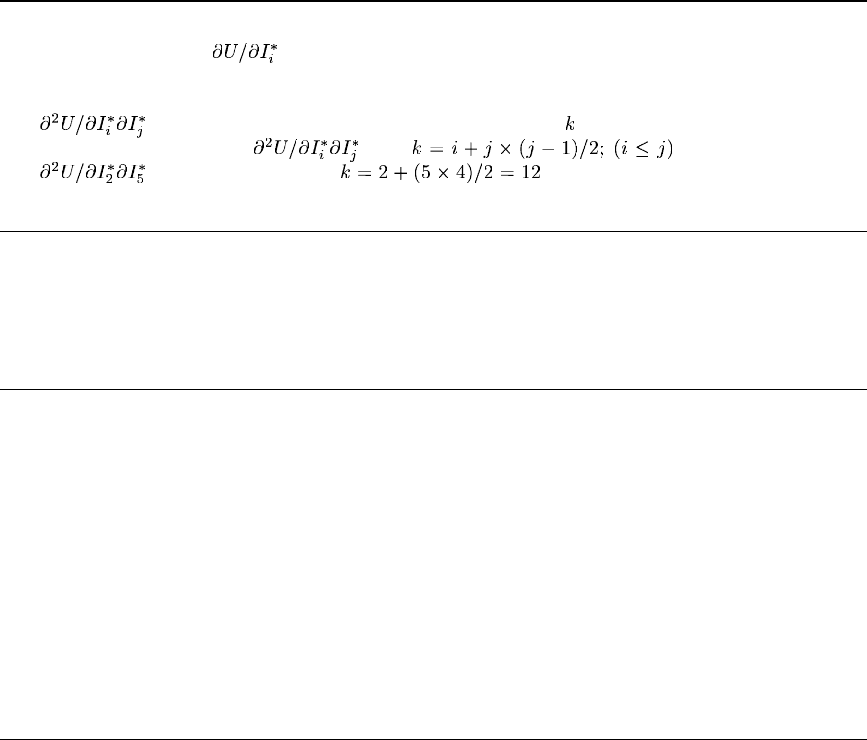
VUANISOHYPER_INV
Storage of arrays of derivatives of energy function
The components of the array duDi of first derivatives of the strain energy potential with respect to
the scalar invariants,
, are stored using the enumeration scheme discussed above for the scalar
invariants.
The elements of the array d2uDiDi of second derivatives of the strain energy function,
, are laid out in memory using triangular storage: if denotes the component in this array
correspondingtotheterm
,then . For example, the term
is stored in component in the d2uDiDi array.
Special considerations for shell elements
When VUANISOHYPER_INV is used to define the material response of shell elements, Abaqus/Explicit
cannot calculate a default value for the transverse shear stiffness of the element. Hence, you must define
the element’s transverse shear stiffness. See “Shell section behavior,” Section 26.6.4 of the Abaqus
Analysis User’s Manual, for guidelines on choosing this stiffness.
Material point deletion
Material points that satisfy a use r-defined failure criterion can be deleted from the model (see
“User-defined mechanical material behavior,” Section 23.8.1 of the Abaqus Analysis U ser’s Manual).
You must specify the state variable number controlling the element deletion flag when you allocate
space for the solution-dependent state variables, as explained in “User-defined mechanical material
behavior,” Section 23.8.1 of the Abaqus Analysis User’s Manual. The deletion stat e variable should
be set to a value of on e or zero in VUANISOHYPER_INV. A value of one indicates that the material
point is active, and a value of zero indicates that Abaqus/Explicit should delete the material point from
the model by setting the stresses to zero. The structure of the block of material points passed to user
subroutine VUANISOHYPER_INV remains unchanged during the a nalysis; deleted mater ial points
are not removed from the block. A baqus/Explicit will “freeze” the values of the invariants passed to
VUANISOHYPER_INV for all deleted material points; that is, the values remain constant after deletion
is triggered. Once a material point has been flagged as deleted, it cannot be reactivated.
User subroutine interface
subroutine vuanisohyper_inv (
C Read only (unmodifiable) variables –
1 nblock, nFiber, nInv,
2 jElem, kIntPt, kLayer, kSecPt,
3 cmname,
4 nstatev, nfieldv, nprops,
5 props, tempOld, tempNew, fieldOld, fieldNew,
6 stateOld, sInvariant, zeta,
C Write only (modifiable) variables –
1.2.8–3
Abaqus ID:
Printed on:

VUANISOHYPER_INV
7 uDev, duDi, d2uDiDi,
8 stateNew )
C
include 'vaba_param.inc'
C
dimension props(nprops),
1 tempOld(nblock),
2 fieldOld(nblock,nfieldv),
3 stateOld(nblock,nstatev),
4 tempNew(nblock),
5 fieldNew(nblock,nfieldv),
6 sInvariant(nblock,nInv),
7 zeta(nblock,nFiber*(nFiber-1)/2),
8 uDev(nblock), duDi(nblock,nInv),
9 d2uDiDi(nblock,nInv*(nInv+1)/2),
* stateNew(nblock,nstatev)
C
character*80 cmname
C
do 100 km = 1,nblock
user coding
100 continue
return
end
Variables to be defined
udev(nblock)
, the deviatoric part of the strain energy density of the primary material response. This quantity
is needed only if the current material definition also includes Mullins effect (see “Mullins effect in
rubberlike m aterials,” Section 19.6.1 of the Abaqus Analysis User’s Manual).
duDi(nblock,nInv)
Array of derivatives of strain energy potential with respect to the scalar invariants,
, ordered
using the enum eration scheme discussed above.
d2uDiDi(nblock,nInv*(nInv+1)/2)
Arrays of second derivatives of strain energy potential with respect to the scalar invariants (using
triangular storage),
.
1.2.8–4
Abaqus ID:
Printed on:

VUANISOHYPER_INV
stateNew(nblock,nstatev)
State variables at each material point at the end of the increm ent. You define the size of this array by
allocating space for it (see “User subroutines: overview,” Section 15.1.1 of the Abaqus Analysis User ’s
Manual, for more information).
Variables passed in for information
nblock
Number of material points to be processed in this call to VUANISOHYPER_STRAIN.
nFiber
Number of families of fibers defined for this material.
nInv
Number of sc
alar invariants.
jElem(nblock)
Array of element numbers.
kIntPt
Integration point number.
kLayer
Layer number (for composite shells ).
kSecPt
Section point number within the current layer.
cmname
User-specified material name, left justified. It is passed in as an uppercase character string. Some
internal material models are given names starting with the “ABQ_” character string. To avoid conflict,
you should not use “ABQ_” as the leading string for cmname.
nstatev
Number of user-defined state variables that are associated with this m aterial type (you define this
as described in “Allocating space” in “User subroutines: overview,” Section 15.1.1 of the Abaqus
Analysis User ’s Manual).
nfieldv
Number of user-defined external field variables.
nprops
User-specified number of user-defined material properties.
props(nprops)
User-supplied material properties.
1.2.8–5
Abaqus ID:
Printed on:

VUANISOHYPER_INV
tempOld(nblock)
Tem peratures at each material point at the beginning of the increm ent.
tempNew(nblock)
Tem peratures at each material point at the end of the increm ent.
fieldOld(nblock,nfieldv)
Values of the user-defined field variables at each material point at the beginning of the increment.
fieldNew(nblock,nfieldv)
Values of the user-defined field variables at each material point at the end of the increment.
stateOld(nblock,nstatev)
State variables at each material point at the beginning of the increment.
sInvariant(nblock,nInv)
Array of scalar invariants,
, at each material point at the end of the increm ent. The invariants are
ordered using the enumeration scheme discus sed above.
zeta(nblock,nFiber*(nFiber-1)/2) )
Array of dot product between the directions of different fam ilies of fiber in the reference configuration,
. The array contains the enumerated values using the scheme discussed above.
Example: Using more than one user-defined anisotropic hyperelastic material model
To use more than one user-defined anisotropic hyperelastic material model, the variable cmname can be
tested for different material names inside use r subroutine VUANISOHYPER_INV, as illustrated below:
if (cmname(1:4) .eq. 'MAT1') then
call VUANISOHYPER_INV1(argument_list)
else if (cmname(1:4) .eq. 'MAT2') then
call VUANISOHYPER_INV2(argument_list)
end if
VUANISOHYPER_INV1 and VUANISOHYPER_INV2 are the actual subroutines containing the
anisotropic hyperelastic m odels for each m aterial MAT1 and MAT2, respectively. Subroutine
VUANISOHYPER_INV merely acts as a directory here. The argument list can be the sam e as that
used in subroutine VUANISOHYPER_INV. The material names must be in uppercase characters since
cmname is passed in as an uppercase character string.
Example: Anisotropic hyperelastic model of Kaliske and Schmidt
As an example of the coding of subroutine VUANISOHYPER_INV, consider the model proposed by
Kaliske and Schmidt (2005) for nonlinear anisotropic elasticity with two families of fi bers. The strain
energy function is given by a polynom ial series expansion in the form
1.2.8–6
Abaqus ID:
Printed on:
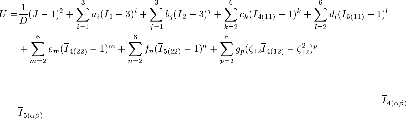
VUANISOHYPER_INV
The code in subroutine VUANISOHYPER_INV must return the derivatives of the strain energy
function with respect to the scalar invariants, w hich are readily computed from the above expression. In
this example auxiliary functions are used to facilitate enumeration of pseudo -invarinats of type
and , as well as for indexing into the array of second derivatives using symmetric storage. The
subroutine would be coded as follows:
subroutine vuanisohyper_inv (
C Read only -
* nblock, nFiber, nInv,
* jElem, kIntPt, kLayer, kSecPt,
* cmname,
* nstatev, nfieldv, nprops,
* props, tempOld, tempNew, fieldOld, fieldNew,
* stateOld, sInvariant, zeta,
C Write only -
* uDev, duDi, d2uDiDi,
* stateNew )
C
include 'vaba_param.inc'
C
dimension props(nprops),
* tempOld(nblock),
* fieldOld(nblock,nfieldv),
* stateOld(nblock,nstatev),
* tempNew(nblock),
* fieldNew(nblock,nfieldv),
* sInvariant(nblock,nInv),
* zeta(nblock,nFiber*(nFiber-1)/2),
* uDev(nblock), duDi(nblock,*),
* d2uDiDi(nblock,*),
* stateNew(nblock,nstatev)
C
character*80 cmname
C
parameter ( zero = 0.d0, one = 1.d0, two = 2.d0,
* three = 3.d0, four = 4.d0, five = 5.d0, six = 6.d0 )
1.2.8–7
Abaqus ID:
Printed on:
VUANISOHYPER_INV
C
C Kaliske energy function (3D)
C
C Read material properties
d=props(1)
dinv = one / d
a1=props(2)
a2=props(3)
a3=props(4)
b1=props(5)
b2=props(6)
b3=props(7)
c2=props(8)
c3=props(9)
c4=props(10)
c5=props(11)
c6=props(12)
d2=props(13)
d3=props(14)
d4=props(15)
d5=props(16)
d6=props(17)
e2=props(18)
e3=props(19)
e4=props(20)
e5=props(21)
e6=props(22)
f2=props(23)
f3=props(24)
f4=props(25)
f5=props(26)
f6=props(27)
g2=props(28)
g3=props(29)
g4=props(30)
g5=props(31)
g6=props(32)
C
dok=1,nblock
Udev(k) = zero
C Compute Udev and 1st and 2nd derivatives w.r.t invariants
C-I1
1.2.8–8
Abaqus ID:
Printed on:
VUANISOHYPER_INV
bi1 = sInvariant(k,1)
term = bi1-three
Udev(k) = Udev(k)
* + a1*term + a2*term**2 + a3*term**3
duDi(k,1) = a1 + two*a2*term + three*a3*term**2
d2uDiDi(k,indx(1,1)) = two*a2 + three*two*a3*term
C-I2
bi2 = sInvariant(k,2)
term = bi2-three
Udev(k) = Udev(k)
* + b1*term + b2*term**2 + b3*term**3
duDi(k,2) = b1 + two*b2*term + three*b3*term**2
d2uDiDi(k,indx(2,2)) = two*b2 + three*two*b3*term
C - I3 (=J)
bi3 = sInvariant(k,3)
term = bi3-one
duDi(k,3) = two*dinv*term
d2uDiDi(k,indx(3,3)) = two*dinv
C - I4(11)
nI411 = indxInv4(1,1)
bi411 = sInvariant(k,nI411)
term = bi411-one
Udev(k) = Udev(k)
* + c2*term**2 + c3*term**3 + c4*term**4
* + c5*term**5 + c6*term**6
duDi(k,nI411) =
* two*c2*term
* + three*c3*term**2
* + four*c4*term**3
* + five*c5*term**4
* + six*c6*term**5
d2uDiDi(k,indx(nI411,nI411)) =
* two*c2
* + three*two*c3*term
* + four*three*c4*term**2
* + five*four*c5*term**3
* + six*five*c6*term**4
C - I5(11)
nI511 = indxInv5(1,1)
bi511 = sInvariant(k,nI511)
term = bi511-one
Udev(k) = Udev(k)
1.2.8–9
Abaqus ID:
Printed on:
VUANISOHYPER_INV
* + d2*term**2 + d3*term**3 + d4*term**4
* + d5*term**5 + d6*term**6
duDi(k,nI511) =
* two*d2*term
* + three*d3*term**2
* + four*d4*term**3
* + five*d5*term**4
* + six*d6*term**5
d2uDiDi(k,indx(nI511,nI511)) =
* two*d2
* + three*two*d3*term
* + four*three*d4*term**2
* + five*four*d5*term**3
* + six*five*d6*term**4
C - I4(22)
nI422 = indxInv4(2,2)
bi422 = sInvariant(k,nI422)
term = bi422-one
Udev(k) = Udev(k)
* + e2*term**2 + e3*term**3 + e4*term**4
* + e5*term**5 + e6*term**6
duDi(k,nI422) =
* two*e2*term
* + three*e3*term**2
* + four*e4*term**3
* + five*e5*term**4
* + six*e6*term**5
d2uDiDi(k,indx(nI422,nI422)) =
* two*e2
* + three*two*e3*term
* + four*three*e4*term**2
* + five*four*e5*term**3
* + six*five*e6*term**4
C - I5(22)
nI522 = indxInv5(2,2)
bi522 = sInvariant(k,nI522)
term = bi522-one
Udev(k) = Udev(k)
* + f2*term**2 + f3*term**3 + f4*term**4
* + f5*term**5 + f6*term**6
duDi(k,nI522) =
* two*f2*term
1.2.8–10
Abaqus ID:
Printed on:
VUANISOHYPER_INV
* + three*f3*term**2
* + four*f4*term**3
* + five*f5*term**4
* + six*f6*term**5
d2uDiDi(k,indx(nI522,nI522)) =
* two*f2
* + three*two*f3*term
* + four*three*f4*term**2
* + five*four*f5*term**3
* + six*five*f6*term**4
C - I4(12)
nI412 = indxInv4(1,2)
bi412 = sInvariant(k,nI412)
term = zeta(k,1)*(bi412-zeta(k,1))
Udev(k) = Udev(k)
* + g2*term**2 + g3*term**3
* + g4*term**4 + g5*term**5
* + g6*term**6
duDi(k,nI412) = zeta(k,1) * (
* two*g2*term
* + three*g3*term**2
* + four*g4*term**3
* + five*g5*term**4
* + six*g6*term**5 )
d2uDiDi(k,indx(nI412,nI412)) = zeta(k,1)**2 * (
* two*g2
* + three*two*g3*term
* + four*three*g4*term**2
* + five*four*g5*term**3
* + six*five*g6*term**4 )
C
end do
C
return
end
C
C Function to map index from Square to Triangular storage
C of symmetric matrix
C
integer function indx( i, j )
include 'vaba_param.inc'
ii = min(i,j)
1.2.8–11
Abaqus ID:
Printed on:

VUANISOHYPER_INV
jj = max(i,j)
indx = ii + jj*(jj-1)/2
return
end
C
C Function to generate enumeration of scalar
C Pseudo-Invariants of type 4
C integer function indxInv4( i, j )
include 'vaba_param.inc'
ii = min(i,j)
jj = max(i,j)
indxInv4=4+jj*(jj-1) + 2*(ii-1)
return
end
C
C Function to generate enumeration of scalar
C Pseudo-Invariants of type 5
C
integer function indxInv5( i, j )
include 'vaba_param.inc'
ii = min(i,j)
jj = max(i,j)
indxInv5=5+jj*(jj-1) + 2*(ii-1)
return
end
Additional reference
•
Kaliske, M., and J. Schmidt, “Formulation of Finite Nonlinear Anisotropic Elasticity,” CADFEM
GmbH Infoplaner 2/2005, vol. 2, pp. 22–23, 2005.
1.2.8–12
Abaqus ID:
Printed on:

VUANISOHYPER_STRAIN
1.2.9 VUANISOHYPER_STRAIN: User subroutine to define anisotropic hyperelastic
material behavior based on Green strain.
Product:
Abaqus/Explicit
References
•
“Anisotropic hyperelastic behavior,” Section 19.5.3 of the Abaqus Analysis User’s Manual
• *
ANISOTROPIC HYPERELASTIC
•
“UANISOHYPER_INV and VUANISOHYPER_INV,” Section 4.1.13 of the Abaqus Verification
Manual
Overview
User subroutine VUANISOHYPER_STRAIN:
•
can be used to define the stra in energy potential of anisotropic hype relastic materials as a f unction
of the components of the Green str ain tensor;
•
will be called for blocks of m aterial calculation points for which the material definition contains
user-defined anisotropic hyperelastic behavior with Green strain-based formulation (“Anisotropic
hyperelastic behavior,” Section 19 .5.3 of the Abaqus Analysis User’s Manual);
•
can use and update solution-dependent state variables;
•
can use any field variables that are passed in; and
•
requires that the values of the derivatives of the strain energy density function be defined with respect
to the components of the modified Green strain tensor and the volume ratio.
Component ordering in tensors
The component ordering depends upon whether the tensor is s econd or fourth order.
Symmetric second-order tensors
For sym metric second-order tensors, such as the modified Green strain tensor, there are ndir+nshr
components; the component order is given as a natural perm utation of the indices of the tensor. The direct
components are first and then the indirect com ponents, beginning w ith the 12-component. For example,
a stress tensor contains ndir direct stress components and nshr shear stress com ponents, w hich are
passedinas
Component 2-D Case 3-D Case
1
2
1.2.9–1
Abaqus ID:
Printed on:

VUANISOHYPER_STRAIN
Component 2-D Case 3-D Case
3
4
5
6
The shear strain com ponents are stored as tensor components and not as engineering components.
Symmetric fourth-order tensors
For sym m etric fourth-order tensors, such as the deviatoric elasticity tensor ,thereare
(ndir+nshr)*(ndir+nshr+1)/2 independent components. These components are orde red using
the following triangular storage scheme:
Component 2-D Case 3-D Case
1
2
3
4
5
6
7
8
9
10
11
12
13
14
15
16
1.2.9–2
Abaqus ID:
Printed on:

VUANISOHYPER_STRAIN
Component 2-D Case 3-D Case
17
18
19
20
21
If Q denotes the component number of term in the above table and M and N (with
) denote the component numbers of and , respectively, in the table for second-order
tensors, Q is given by the relationship
. For example, consider the term
. The component numbers for and are and , respectively, giving
.
Special consideration for shell elements
When VUANISOHYPER_STRAIN is used to define the material response of shell elements,
Abaqus/Explicit cannot calculate a default value for the transverse shear stiffness of the element. H ence,
you must define the element’s transverse shear stiffness. See “Shell section behavior,” Section 26.6.4 of
the Abaqus Analysis User’s Manual, for guidelines on choosing this stiffness.
Material point deletion
Material points that satisfy a use r-defined failure criterion can be deleted from the model (see
“User-defined mechanical material behavior,” Section 23.8.1 of the Abaqus Analysis U ser’s Manual).
You must specify the state variable number controlling the element deletion flag when you allocate
space for the solution-dependent state variables, as explained in “User-defined mechanical material
behavior,” Section 23.8.1 of th e Abaqus Analysis User’s Manual. The deletion state variable should be
set to a value of one or zero in VUANISOHYPER_STRAIN. A value of one indicates that the material
point is active, and a value of zero indicates that Abaqus/Explicit should delete the material point
from the model by setting the stresses to zero. The structure of the block of material poi nts pa ssed to
user subroutine VUANISOHYPER_STRAIN remains unchanged during the analysis; deleted material
points are not rem oved from the block. Abaqus/Explicit will “freeze” the values of the strains passed
to VUANISOHYPER_STRAIN for all deleted materi al points; that is, the strain values remain constant
after deletion is triggered. Once a material point has been flagged as deleted, it cannot be reactivated.
User subroutine interface
subroutine vuanisohyper_strain(
C Read only (unmodifiable) variables –
1 nblock,jElem,kIntPt,kLayer,kSecPt,cmname,
1.2.9–3
Abaqus ID:
Printed on:

VUANISOHYPER_STRAIN
2 ndir,nshr,nstatev,nfieldv,nprops,
3 props,tempOld,tempNew,fieldOld,fieldNew,
4 stateOld,ebar,detu,
C Write only (modifiable) variables –
4 udev,duDe,duDj,
5 d2uDeDe,d2uDjDj,d2uDeDj,
6 stateNew)
C
include 'vaba_param.inc'
C
dimension jElem(nblock),
1 props(nprops),
2 tempOld(nblock),
3 fieldOld(nblock,nfieldv),
4 stateOld(nblock,nstatev),
5 tempNew(nblock),
6 fieldNew(nblock,nfieldv),
7 ebar(nblock,ndir+nshr), detu(nblock),
8 uDev(nblock),
9 duDe(nblock,ndir+nshr), duDj(nblock),
* d2uDeDe(nblock,(ndir+nshr)*(ndir+nshr+1)/2),
1 d2uDjDj(nblock),
2 d2uDeDj(nblock,ndir+nshr),
3 stateNew(nblock,nstatev)
C
character*80 cmname
C
do 100 km = 1,nblock
user coding
100 continue
return
end
Variables to be defined
udev(nblock)
, the deviatoric part of the strain energy density of the primary material response. This quantity
is needed only if the current material definition also includes Mullins effect (see “Mullins effect in
rubberlike m aterials,” Section 19.6.1 of the Abaqus Analysis User’s Manual).
1.2.9–4
Abaqus ID:
Printed on:

VUANISOHYPER_STRAIN
duDe(nblock,ndir+nshr)
Derivatives of strain energy potential with respect to the components of the modified Green strain
tensor,
.
duDj(nblock,ndir+nshr)
Derivatives of strain energy potential with respect to volume ratio, .
d2uDeDe(nblock,(ndir+nshr)*(ndir+nshr+1)/2)
Second derivatives of strain energy potential with respect to the co mponents of the modified Green
strain tensor (using triangular storage),
.
d2uDjDj(nblock)
Second derivatives of strain energy potential with respect to volume ratio, .
d2uDeDj(nblock,ndir+nshr)
Cross derivatives of strain energy potential with respect to components of the mo dified Green strain
tensor and volume ratio,
.
stateNew(nblock,nstatev)
State variables at each material point at the end of the increm ent. You define the size of this array by
allocating space for it (see “User subroutines: overview,” Section 15.1.1 of the Abaqus Analysis User ’s
Manual, for more information).
Variables passed in for information
nblock
Number of material points to be processed in this call to VUANISOHYPER_STRAIN.
jElem(nblock)
Array of element numbers.
kIntPt
Integration point number.
kLayer
Layer number (for composite shells ).
kSecPt
Section point number within the current layer.
cmname
User-specified material name, left justified. It is passed in as an uppercase character string. Some
internal material models are given names starting with the “ABQ_” character string. To avoid conflict,
you should not use “ABQ_” as the leading string for cmname.
1.2.9–5
Abaqus ID:
Printed on:

VUANISOHYPER_STRAIN
ndir
Number of direct components i n a symmetric tensor.
nshr
Number of indirect components in a symmetric tensor.
nstatev
Number of user-defined state variables that are associated with this m aterial type (you define this
as described in “Allocating space” in “User subroutines: overview,” Section 15.1.1 of the Abaqus
Analysis User ’s Manual).
nfieldv
Number of user-defined external field variables.
nprops
User-specified number of user-defined material properties.
props(nprops)
User-supplied material properties.
tempOld(nblock)
Tem peratures at each material point at the beginning of the increm ent.
tempNew(nblock)
Tem peratures at each material point at the end of the increm ent.
fieldOld(nblock,nfieldv)
Values of the user-defined field variables at each material point at the beginning of the increment.
fieldNew(nblock,nfieldv)
Values of the user-defined field variables at each material point at the end of the increment.
stateOld(nblock,nstatev)
State variables at each material point at the beginning of the increment.
ebar(nblock,ndir+nshr)
Modified Green strain tensor,
, at each material point at the end of the increment.
detu(nblock)
J, determinant of deformation gradient (volume ratio) at the end of the increment.
Example: Using more than one user-defined anisotropic hyperelastic material model
To use more than one user-defined anisotropic hyperelastic material model, the variable cmname can
be tested for different material names inside user subroutine VUANISOHYPER_STRAIN, as illustrated
below:
1.2.9–6
Abaqus ID:
Printed on:

VUANISOHYPER_STRAIN
if (cmname(1:4) .eq. 'MAT1') then
call VUANISOHYPER_STRAIN1(argument_list)
else if (cmname(1:4) .eq. 'MAT2') then
call VUANISOHYPER_STRAIN2(argument_list)
end if
VUANISOHYPER_STRAIN1 and VUANISOHYPER_STRAIN2 are the actual subroutines containing
the anisotropic hyperelastic models for each material MAT1 and MAT2, respectively. Subroutine
VUANISOHYPER_STRAIN merely acts as a directory here. The argument list can be the same as that
used in subroutine VUANISOHYPER_STRAIN. The material names must be in uppercase characters
since cmname is passed in as an uppercase character string.
Example: Orthotropic Saint-Venant Kirchhoff model
As a simple example of the coding of subroutine VUANISOHYPER_STRAIN, consider the
generalization to anisotropic hypere lasticity of the Sa int-Venant Kirchhoff model. The strain energy
function of the Saint-Venant Kirchhoff model can be expressed as a quadratic function of the Green
strain tensor,
,as
where is the fourth-order elasticity tensor. The derivatives of the strain energy function with respect
to the G reen strain are given as
However, subroutine VUANISOHYPER_STRAIN must return the derivatives of the stra in energy
function with respect to the modified Green strain tensor,
, and the volume rati o, J, which can be
accomplished easily using the following relationship between
, ,and :
where is the second-order identity tensor. Thus, using the chain rule we find
1.2.9–7
Abaqus ID:
Printed on:

VUANISOHYPER_STRAIN
where
and
In this example an auxiliary function is used to facilitate indexing into a fourth-order symmetric
tensor. The subroutine would be coded as follows:
subroutine vuanisohyper_strain (
C Read only -
* nblock,
* jElem, kIntPt, kLayer, kSecPt,
* cmname,
* ndir, nshr, nstatev, nfieldv, nprops,
* props, tempOld, tempNew, fieldOld, fieldNew,
* stateOld, ebar, detu,
C Write only -
* uDev, duDe, duDj,
* d2uDeDe, d2uDjDj, d2uDeDj,
* stateNew )
C
include 'vaba_param.inc'
C
dimension props(nprops),
* tempOld(nblock),
* fieldOld(nblock,nfieldv),
* stateOld(nblock,nstatev),
* tempNew(nblock),
* fieldNew(nblock,nfieldv),
* ebar(nblock,ndir+nshr), detu(nblock),
1.2.9–8
Abaqus ID:
Printed on:
VUANISOHYPER_STRAIN
* uDev(nblock), duDe(nblock,ndir+nshr), duDj(nblock),
* d2uDeDe(nblock,*), d2uDjDj(nblock),
* d2uDeDj(nblock,ndir+nshr),
* stateNew(nblock,nstatev)
C
character*80 cmname
C
parameter( half = 0.5d0, one = 1.d0, two = 2.d0,
* third = 1.d0/3.d0, twothds = 2.d0/3.d0, four = 4.d0,
* dinv = 0.d0 )
C
C Orthotropic Saint-Venant Kirchhoff strain energy function
C (3D)
C
D1111 = props(1)
D1122 = props(2)
D2222 = props(3)
D1133 = props(4)
D2233 = props(5)
D3333 = props(6)
D1212 = props(7)
D1313 = props(8)
D2323 = props(9)
C
dok=1,nblock
C
d2UdE11dE11 = D1111
d2UdE11dE22 = D1122
d2UdE11dE33 = D1133
d2UdE22dE11 = d2UdE11dE22
d2UdE22dE22 = D2222
d2UdE22dE33 = D2233
d2UdE33dE11 = d2UdE11dE33
d2UdE33dE22 = d2UdE22dE33
d2UdE33dE33 = D3333
d2UdE12dE12 = D1212
d2UdE13dE13 = D1313
d2UdE23dE23 = D2323
C
xpow = exp ( log(detu(k)) * twothds )
detuInv = one / detu(k)
C
1.2.9–9
Abaqus ID:
Printed on:
VUANISOHYPER_STRAIN
E11 = xpow * ebar(k,1) + half * ( xpow - one )
E22 = xpow * ebar(k,2) + half * ( xpow - one )
E33 = xpow * ebar(k,3) + half * ( xpow - one )
E12 = xpow * ebar(k,4)
E23 = xpow * ebar(k,5)
E13 = xpow * ebar(k,6)
C
term1 = twothds * xpow * detuInv
dE11Dj = term1 * ( E11 + half )
dE22Dj = term1 * ( E22 + half )
dE33Dj = term1 * ( E33 + half )
dE12Dj = term1 * E12
dE13Dj = term1 * E13
dE23Dj = term1 * E23
term2 = - third * detuInv
d2E11DjDj = term2 * dE11Dj
d2E22DjDj = term2 * dE22Dj
d2E33DjDj = term2 * dE33Dj
d2E12DjDj = term2 * dE12Dj
d2E13DjDj = term2 * dE13Dj
d2E23DjDj = term2 * dE23Dj
C
dUdE11 = d2UdE11dE11 * E11
* + d2UdE11dE22 * E22
* + d2UdE11dE33 * E33
dUdE22 = d2UdE22dE11 * E11
* + d2UdE22dE22 * E22
* + d2UdE22dE33 * E33
dUdE33 = d2UdE33dE11 * E11
* + d2UdE33dE22 * E22
* + d2UdE33dE33 * E33
dUdE12 = two * d2UdE12dE12 * E12
dUdE13 = two * d2UdE13dE13 * E13
dUdE23 = two * d2UdE23dE23 * E23
C
U = half * ( E11*dUdE11 + E22*dUdE22 + E33*dUdE33 )
* + E12*dUdE12 + E13*dUdE13 + E23*dUdE23
uDev(k) = U
C
duDe(k,1) = xpow * dUdE11
duDe(k,2) = xpow * dUdE22
duDe(k,3) = xpow * dUdE33
1.2.9–10
Abaqus ID:
Printed on:
VUANISOHYPER_STRAIN
duDe(k,4) = xpow * dUdE12
duDe(k,5) = xpow * dUdE23
duDe(k,6) = xpow * dUdE13
C
xpow2 = xpow * xpow
C Only update nonzero components
d2uDeDe(k,indx(1,1)) = xpow2 * d2UdE11dE11
d2uDeDe(k,indx(1,2)) = xpow2 * d2UdE11dE22
d2uDeDe(k,indx(2,2)) = xpow2 * d2UdE22dE22
d2uDeDe(k,indx(1,3)) = xpow2 * d2UdE11dE33
d2uDeDe(k,indx(2,3)) = xpow2 * d2UdE22dE33
d2uDeDe(k,indx(3,3)) = xpow2 * d2UdE33dE33
d2uDeDe(k,indx(4,4)) = xpow2 * d2UdE12dE12
d2uDeDe(k,indx(5,5)) = xpow2 * d2UdE23dE23
d2uDeDe(k,indx(6,6)) = xpow2 * d2UdE13dE13
*
duDj(k) = dUdE11*dE11Dj + dUdE22*dE22Dj + dUdE22*dE22Dj
* + two * ( dUdE12*dE12Dj + dUdE13*dE13Dj
* + dUdE23*dE23Dj )
d2uDjDj(k)= dUdE11*d2E11DjDj+dUdE22*d2E22DjDj
* +dUdE22*d2E22DjDj
* + two*(dUdE12*d2E12DjDj+dUdE13*d2E13DjDj
* +dUdE23*d2E23DjDj)
* + d2UdE11dE11 * dE11Dj * dE11Dj
* + d2UdE22dE22 * dE22Dj * dE22Dj
* + d2UdE33dE33 * dE33Dj * dE33Dj
* + two * ( d2UdE11dE22 * dE11Dj * dE22Dj
* + d2UdE11dE33 * dE11Dj * dE33Dj
* + d2UdE22dE33 * dE22Dj * dE33Dj )
* + four * ( d2UdE12dE12 * dE12Dj * dE12Dj
* d2UdE13dE13 * dE13Dj * dE13Dj
* d2UdE23dE23 * dE23Dj * dE23Dj )
* d2uDeDj(k,1) = term1 * dUdE11 + xpow * (
* d2UdE11dE11 * dE11Dj
* + d2UdE11dE22 * dE22Dj
* + d2UdE11dE33 * dE33Dj )
d2uDeDj(k,2) = term1 * dUdE22 + xpow * (
* d2UdE22dE11 * dE11Dj
* + d2UdE22dE22 * dE22Dj
* + d2UdE22dE33 * dE33Dj )
d2uDeDj(k,3) = term1 * dUdE33 + xpow * (
* + d2UdE33dE11 * dE11Dj
1.2.9–11
Abaqus ID:
Printed on:
VUANISOHYPER_STRAIN
* + d2UdE33dE22 * dE22Dj
* + d2UdE33dE33 * dE33Dj )
d2uDeDj(k,4) = term1 * dUdE12
* + xpow * two * d2UdE12dE12 * dE12Dj
d2uDeDj(k,5) = term1 * dUdE23
* + xpow * two * d2UdE23dE23 * dE23Dj
d2uDeDj(k,6) = term1 * dUdE13
* + xpow * two * d2UdE13dE13 * dE13Dj
end do
C
return
end
C
integer function indx( i, j )
C
include 'vaba_param.inc'
C
C Function to map index from Square to Triangular storage
C of symmetric matrix
C
ii = min(i,j)
jj = max(i,j)
C
indx = ii + jj*(jj-1)/2
C
return
end
1.2.9–12
Abaqus ID:
Printed on:

VUEL
1.2.10 VUEL: User subroutine to define an element.
Product:
Abaqus/Explicit
WARNING: This feature is intended f or advanced users only. Its use in all but the
simplest test examples will require considerable coding by the user/developer.
“User-defined elements,” Section 29.16.1 of the Abaqus Analysis User’s Manual,
should be read before proceeding.
References
•
“User-defined elements,” Section 29.16.1 of the Abaqus A nalysis User’s Manual
•
“User-defined element library,” Section 29.16.2 of the Abaqus Analysis User’s Manual
•
“UEL,” Section 1.1.23
• *
UEL PROPERTY
• *
USER ELEMENT
Overview
User subroutine VUEL:
•
will be called for each element that is of a general user-defined elem ent type each time element
calculations are required; and
•
(or subroutines called by user subroutine VUEL) must perform all of the calculations for the element,
appropriate to the current activity in the analysis.
User subroutine interface
SUBROUTINE VUEL(nblock,rhs,amass,dtimeStable,svars,nsvars,
1 energy,
2 nnode,ndofel,props,nprops,jprops,njprops,
3 coords,mcrd,u,du,v,a,
4 jtype,jElem,
5 time,period,dtimeCur,dtimePrev,kstep,kinc,
6 lflags,
7 dMassScaleFactor,
8 predef,npredef,
9 jdltyp, adlmag)
C
include 'vaba_param.inc'
C operational code keys
1.2.10–1
Abaqus ID:
Printed on:
VUEL
parameter ( jMassCalc = 1,
* jIntForceAndDtStable = 2,
* jExternForce = 3)
C flag indices
parameter (iProcedure = 1,
* iNlgeom = 2,
* iOpCode = 3,
* nFlags = 3)
C energy array indices
parameter ( iElPd = 1,
* iElCd = 2,
* iElIe = 3,
* iElTs = 4,
* iElDd = 5,
* iElBv = 6,
* iElDe = 7,
* iElHe = 8,
* iElKe = 9,
* iElTh = 10,
* iElDmd = 11,
* iElDc = 12,
* nElEnergy = 12)
C predefined variables indices
parameter ( iPredValueNew = 1,
* iPredValueOld = 2,
* nPred = 2)
C time indices
parameter (iStepTime = 1,
* iTotalTime = 2,
* nTime = 2)
dimension rhs(nblock,ndofel),amass(nblock,ndofel,ndofel),
1 dtimeStable(nblock),
2 svars(nblock,nsvars),energy(nblock,nElEnergy),
3 props(nprops),jprops(njprops),
4 jElem(nblock),time(nTime),lflags(nFlags),
5 coords(nblock,nnode,mcrd),
6 u(nblock,ndofel), du(nblock,ndofel),
1.2.10–2
Abaqus ID:
Printed on:

VUEL
7 v(nblock,ndofel), a(nblock, ndofel),
8 dMassScaleFactor(nblock),
9 predef(nblock,nnode,npredef,nPred),
* adlmag(nblock)
do kblock = 1,nblock
user coding to define rhs, amass, dtimeStable, svars and energy
end do
RETURN
END
Variables to be defined
Some of the following arrays depend on the value of the lflags array.
rhs
An array containing the contributions of each element to the right-hand-side vector of the overall system
of equations. Depending on the settings of the lflags array, it contains either the internal force from
the element or the external load calculated from the specified distributed loads.
amass
An array containing the contribution of each element to the m ass matrix of the overall system of
equations.
All nonzero entries in amass should be defined. Moreover, the mass matrix must be symmetric.
There are several other requirements that apply depending on the active degrees of freedom specified.
These requirements are explained in detail below.
dtimeStable
A scalar value defining, for each element, the upper limit of the time increment for stability
considerations. This would be the maximum time in crement to be used in the subsequent increment
for this element to be stable (to satisfy the C ourant condition). This value depends strongly on the
element formulation, and it is important that is comput ed appropriately.
svars
An array containing the values of the solution-dependent state variables associated with each element.
The number of such variables is nsvars (see below). You define the meaning of these variables.
This array is passed into VUEL containing the values of these variables at the start of the current
increment. In most cases they should be updated to be the values at the end of the increment. In rare
cases such an update is not required.
energy
The array energy contains the values of the energy quantities associated with each element. The
values in this array when VUEL is called are the element energy quantities at the start of the current
1.2.10–3
Abaqus ID:
Printed on:

VUEL
increment. They should be updated to the correct values at the end of the current increment; otherwise,
plots of the energy balance for the entire model will not be accurate. Depending on the elem ent
formulation, many of these energies could be zero at all times. The entries in the array are as follows:
energy(nblock,iElPd ) Plastic dissipation.
energy(nblock,iElCd) Creep dissipation.
energy(nblock,iElIe) Internal energy.
energy(nblock,iElTs) Transverse shear energy.
energy(nblock,iElDd) Material damping
dissipation.
energy(nblock,iElBv) Bulk viscosity
dissipation.
energy(nblock,iElDe) Drill energy.
energy(nblock,iElHe) Hourglass energy.
energy(nblock,iElKe) Kinetic energy.
energy(nblock,iElTh) Heat energy.
energy(nblock,iElDmd) Damage dissipation.
energy(nblock,iElDc ) Distortion control
energy.
Variables passed in for information
Arrays:
props
A floating point array c ontaining the nprops real property values defined for use with each element
processed. nprops is the user-specified number of real property values. See “Defining the element
properties” in “User-defined elements,” Section 29.16.1 of the Abaqus Analysis User’s Manual.
jprops
An integer array containing the njprops integer property values defined for use with each element
processed. njprops is the user-specified number of integer property values. See “D efining the
element properties” in “User-defined elem ents,” Section 29.16.1 of the Abaqus Analysis User’s
Manual.
coords
An array containing the original coordina tes of the nodes of the elemen t. coords(kblock,k1,k2)
is the k2th coordinate of the k1th nod e of the kblock element.
1.2.10–4
Abaqus ID:
Printed on:
VUEL
u, du, v, a
Arrays containing the basic solution variables (displacements, rotations, temperatures, pressures,
depending on the degree of freedom) at the nodes of the element. Values a re provided as follows,
illustrated below for the k1th degree of freedom of the kblock element:
u(kblock,k1) Total value of the variables (such as
displacements or rotations) at the end of
the current increment.
du(kblock,k1) Incremental values of the variables in the
current increment.
v(kblock,k1) Time rate of change of the variables
(velocities, rates of rotation) at the
midpoint of the increment.
a(kblock,k1) Accelerations of the variables at the end
of the current increment.
jElem
jElem(kblock) contains the element nu mber for the kblock elem ent.
adlmag
adlmag(kblock) is the total load magnitude of the load type jdltyp (integer identifying the load
number for distributed load type Un) distributed load at the end of the current increment for distributed
loads of type Un.
predef
An array containing the values of predefined field variables, such as temperature in an uncoupled
stress/displacement analysis, at the nodes of the elem ent (“Predefined fields,” Section 30.6.1 of the
Abaqus Analysis User’s Manual).
The second index, k2, indicates the local node number on the kblock element. The third index,
k3, indicates the variable: the temperature is stored if the index is 1, and the predefined field variables
are stored if the indices are greater than or equal to 2. The fourth index of the array, k4, is either 1 or
2, with 1 indica ting the value of the field va riable at the end of the increment and 2 indicating the value
of the field variable at the beginning of the increment.
predef(kblock,k2,1,k4) Temperature.
predef(kblock,k2,2,k4) First predefined field variable.
predef(kblock,k2,3,k4) Second predefined field variable.
Etc. Any other predefined field
variable.
1.2.10–5
Abaqus ID:
Printed on:
VUEL
predef(kblock,k2,k3,k4) Val u e of the (k3–1)th predefined
field variable at the k2th node of
the element at the beginning or
the end of the increment.
predef(kblock,k2,k3,1) Values of the variables at the end
of the current increment.
predef(kblock,k2,k3,2) Values of the variables at
the beginning of the current
increment.
lflags
An array containing the flags that defi ne the current solution procedure and requirements for element
calculations.
lflags(iProcedure) Defines the procedure type. See
“Results file output format,”
Section 5.1.2 of the Abaqus Analysis
User’s Manual, for the key used for
each procedure.
lflags(iNlgeom)=0 Small-displacement analysis.
lflags(iNlgeom)=1 Large-displacement analysis (nonlinear
geometric effects included in the step;
see “General and linear perturba tion
procedures,” Section 6.1.2 of the
Abaqus Analysis User’s Manual).
lflags(iOpCode)=jMassCalc Define the mass matrix amass in the
beginning of the analysis.
lflags(iOpCode)=jIntForceAnd-
DtStable
Define the element internal force.
Define the stable time increment as
well.
lflags(iOpCode)=jExternForce Define the distributed load effect on
the external force associated with the
element.
dMassScaleFactor
An array containing the mass scale factors for each element.
time(iStepTime)
Current value of step time.
1.2.10–6
Abaqus ID:
Printed on:
VUEL
time(iTotalTime)
Current value of total time.
Scalar parameters:
nblock
Number of user elements to be processed in this call to VUEL.
dtimeCur
Current tim e increment.
dtimePrev
Previous time increment.
period
Time period of the current s tep.
ndofel
Number of degrees of freedom in the elements processed.
nsvars
User-defined number of solution- dependent state varia bles a ssociated wi th the element (“Defin ing
the number of solution-dependent variables that m ust be stored within the element” in “User-defined
elements,” Section 29.16.1 of the Abaqus Analysis User’s Manual).
nprops
User-defined number of real property values associated with the elements processed (“Defining the
element properties” in “User-defined elem ents,” Section 29.16.1 of the Abaqus Analysis User’s
Manual).
njprops
User-defined number of integer property values associated with the elements processed (“Defining
the element properties” in “User-defined elements,” Section 29.16.1 of the A baqus Analysis User’s
Manual).
mcrd
mcrd is defined as the maximum of the user-defined maximum number of coordinates needed at any
node point (“Defining the maxim um number of coordinates needed at any nodal point” in “User-defined
elements,” Section 29.16.1 of the Abaqus Analysis U ser’s Manual) and the value of the largest active
degree of freedom of the user elem ent that is less than or equal to 3. For example, if you specify that
the maximum num ber of coordinates is 1 and the active degrees of freedom of the user element are 2,
3, and 6 mcrd will be 3. If y ou specify that the maximum number of coordinates is 2 and the active
degree of freedom of the us er element is 11, mcrd will be 2.
1.2.10–7
Abaqus ID:
Printed on:

VUEL
nnode
User-defined number of nodes on the elements (“Defining the num ber of nodes associated with the
element” in “User-defined elements,” Section 29.16.1 of the Abaqus A nalysis User’s Manual).
jtype
Integer defining the eleme nt ty pe. This is the user-defined integer value n in elem ent type
VUn (“Assigning an element type key to a user-defined element” in “User-defined elements,”
Section 29.16.1 of the Abaqus Analysis User’s Manual).
kstep
Current step number.
kinc
Current increment number.
npredef
Number of predefined field variables, including temperature. For user elem ents Abaqus/Explicit uses
one value for each field variable per node.
VUEL conventions
The solution variables (displacement, velocity, etc.) are arranged on a node/degree of freedom basis. The
degrees of freedom of the first node are first, followed by the degrees of freedom of the second node, etc.
The degrees of freedom that will be updated automatically in Abaqus/Explicit are: 1–3 (displacements),
4–6 (rotations), 8 (pressure), and 11 (temperature). Depending on the procedure type (see below), only
some of the degrees of freedom listed above will be updated. Other degrees of freedom will not be
updated by the time integra tion procedure in Abaqus/Explicit an d, hence, should not be used.
ThemassmatrixdefinedinusersubroutineVUEL must be symmetric. In addition, the following
requirements apply:
•
The m ass m atrix entries associated with the translational degrees of freedom for a particular node
must be diagonal. Moreover, these diagonal entries must be equal to each other.
•
There must be no coupling (off-diagonal) entries specified between degrees of freedom of different
kinds. For example, you cannot specify nonzero mass matrix entries to couple the translational
degrees of freedom to the rotational degrees of freedom.
•
There must be no coupling (off-diagonal) entries specified between degrees of freedom belonging
to different nodes.
You must be using appropriate lumping techniques to provide a mass matrix that foll ows these
requirements. For the rotational degrees of freedom at a pa rticular node in three-dimensional analyses,
you can specify a fully populated symmetric 3 × 3 iner tia tensor.
Usage with general nonlinear procedures
The following illustrates the use in explicit dynamic procedures:
1.2.10–8
Abaqus ID:
Printed on:

VUEL
Direct-integration explicit dynamic analysis (lflags(iProcedure)=17)
•
Automatic updates for degrees of freedom 1–6, 8, and 11.
•
The governing equations are as described in “Explicit dynamic analysis,” Section 6.3.3 of the
Abaqus Analysis User’s Manual.
•
Coding for the operational code lflags(iOpCode)=jExternForceis optional.
Transient fully coupled thermal-stress analysis (lflags(iProcedure)=74)
•
Automatic updates for degrees of freedom 1–6 and 8.
•
The governing equations are as described in “Fully coupled thermal-stress analysis in
Abaqus/Explicit” in “Fully coupled thermal-stress analy sis,” Section 6.5.4 of the Abaqus Analysis
User’s Manual.
•
Coding for the operational code lflags(iOpCode)=jExternForce is optional.
Example: Structural user element
A structural user element has been created t o demonstrate the usage of subroutine VUEL. The se user-
defined elements are applied in a num ber of analyses. The following excerpt is from the verification
problem that invokes the structural user element in an explicit dyna mic procedure:
*
USER ELEMENT, NODES=2, TYPE=VU1, PROPERTIES=4, COORDINATES=3,
VARIABLES=12
1, 2, 3
*
ELEMENT, TYPE=VU1
101, 101, 102
*
ELGEN, ELSET=VUTRUSS
101, 5
*
UEL PROPERTY, ELSET=VUTRUSS
0.002, 2.1E11, 0.3, 7200.
The user element consists of two nodes that are assumed to lie parallel to the x-axis. The element behaves
similarly to a linear truss element. The supplied element properties are the cross-sectional area, Young’s
modulus, Poisson’s ratio, and dens ity, respectively.
The next excerpt shows the listing of the subroutine. The user subroutine has been coded for use
in an explicit dynam ic analysis. The names of the verification input files associated with the subroutine
and these procedures can be found in “VUEL,” Section 4.1.32 of the Abaqus Verification Manual.
subroutine vuel(
* nblock,
* rhs,amass,dtimeStable,
* svars,nsvars,
* energy,
* nnode,ndofel,
1.2.10–9
Abaqus ID:
Printed on:
VUEL
* props,nprops,
* jprops,njprops,
* coords,ncrd,
* u,du,v,a,
* jtype,jElem,
* time,period,dtimeCur,dtimePrev,kstep,kinc,lflags,
* dMassScaleFactor,
* predef,npredef,
* ndload,adlmag)
include 'vaba_param.inc'
c operation code
parameter ( jMassCalc = 1,
* jIntForceAndDtStable = 4)
c flags
parameter (iProcedure = 1,
* iNlgeom = 2,
* iOpCode = 3,
* nFlags = 3)
c procedure flags
parameter ( jDynExplicit = 17 )
c time
parameter (iStepTime = 1,
* iTotalTime = 2,
* nTime = 2)
c energies
parameter ( iElPd = 1,
* iElCd = 2,
* iElIe = 3,
* iElTs = 4,
* iElDd = 5,
* iElBv = 6,
* iElDe = 7,
* iElHe = 8,
* iElKe = 9,
* iElTh = 10,
* iElDmd = 11,
1.2.10–10
Abaqus ID:
Printed on:
VUEL
* iElDc = 12,
* nElEnergy = 12)
parameter (factorStable = 0.99d0)
parameter ( zero = 0.d0, half = 0.5d0, one = 1.d0, two=2.d0 )
C
dimension rhs(nblock,ndofel), amass(nblock,ndofel,ndofel),
* dtimeStable(nblock),
* svars(nblock,nsvars), energy(nblock,nElEnergy),
* props(nprops), jprops(njprops),
* jElem(nblock), time(nTime), l(nFlags),
* coords(nblock,nnode,ncrd), u(nblock,ndofel),
* du(nblock,ndofel), v(nblock,ndofel), a(nblock, ndofel),
* predef(nblock, nnode, npredef, nPred), adlmag(nblock),
* dMassScaleFactor(nblock)
c Notes:
c Define only nonzero entries; the arrays to be defined have
c been zeroed out just before this call
if (jtype .eq. 1001 .and.
* lflags(iProcedure).eq.jDynExplicit) then
area0 = props(1)
eMod = props(2)
anu = props(3)
rho = props(4)
eDampTra = zero
amassFact0 = half*area0*rho
if ( lflags(iOpCode).eq.jMassCalc ) then
do kblock = 1, nblock
c use original distance to compute mass
alenX0 = (coords(kblock,2,1) - coords(kblock,1,1))
alenY0 = (coords(kblock,2,2) - coords(kblock,1,2))
alenZ0 = (coords(kblock,2,3) - coords(kblock,1,3))
alen0 = sqrt(alenX0*alenX0 + alenY0*alenY0 +
* alenZ0*alenZ0)
am0 = amassFact0*alen0
amass(kblock,1,1) = am0
1.2.10–11
Abaqus ID:
Printed on:
VUEL
amass(kblock,2,2) = am0
amass(kblock,3,3) = am0
amass(kblock,4,4) = am0
amass(kblock,5,5) = am0
amass(kblock,6,6) = am0
end do
else if ( lflags(iOpCode) .eq.
* jIntForceAndDtStable) then
do kblock = 1, nblock
alenX0 = (coords(kblock,2,1) - coords(kblock,1,1))
alenY0 = (coords(kblock,2,2) - coords(kblock,1,2))
alenZ0 = (coords(kblock,2,3) - coords(kblock,1,3))
alen0 = sqrt(alenX0*alenX0 + alenY0*alenY0 +
* alenZ0*alenZ0)
vol0 = area0*alen0
amElem0 = two*amassFact0*alen0
alenX = alenX0
* + (u(kblock,4) - u(kblock,1))
alenY = alenY0
* + (u(kblock,5) - u(kblock,2))
alenZ = alenZ0
* + (u(kblock,6) - u(kblock,3))
alen = sqrt(alenX*alenX + alenY*alenY + alenZ*alenZ)
area = vol0/alen
ak = area*eMod/alen
c stable time increment for translations
dtimeStable(kblock) = factorStable*sqrt(amElem0/ak)
c force=E*logarithmic strain *current area
strainLog = log(alen/alen0)
fElasTra = eMod*strainLog*area
forceTra = fElasTra
c assemble internal load in RHS
rhs(kblock,1) = -forceTra
rhs(kblock,4) = forceTra
c internal energy calculation
1.2.10–12
Abaqus ID:
Printed on:
VUEL
alenOld = svars(kblock,1)
fElasTraOld = svars(kblock,2)
energy(kblock, iElIe) = energy(kblock, iElIe) +
* half*(fElasTra+fElasTraOld)*(alen - alenOld)
c update state variables
svars(kblock,1) = alen
svars(kblock,2) = fElasTra
end do
end if
end if
c
return
end
1.2.10–13
Abaqus ID:
Printed on:

VUFIELD
1.2.11 VUFIELD: User subroutine to specify predefined field variables.
Product:
Abaqus/Explicit
References
•
“Predefined fields,” Section 30.6.1 of the Abaqus Analysis User’s Manual
• *
FIELD
Overview
User subroutine VUFIELD:
•
allows you to prescribe predefined field variables at the nodes of a m odel—the predefined field
variables at a node can be update d individually, or a number of field variables at the nodes can be
updated simultaneously;
•
can be called for blocks of nodes for which the field variable values are defined in the subroutine;
•
ignores any field variable values specified directly;
•
can be used to m odify field variable values read from a results file; and
•
can be used in conjunction with user subroutine VUSDFLD such that the field variables that are
passed in from VUFIELD and interpolated to the material points can be modified (such changes are
local to m aterial point values, and nodal field variable values remain unaffected).
Updating field variables
Two different methods are provided for updatin g field variables.
Individual variable updates
By defau lt, only one field var iable is updated at a time for given nodes or a given node set in user
subroutine VUFIELD. The user subroutine is called whenever a current value of a field variable is needed
for the nodes that are listed in the field variable definition. This method is ideal for cas es in which the
field variables are independent of each other.
Simultaneous variable updates
User subroutine VUFIELD can also be used to update multipl e field variables simultaneously for given
nodes or a given node set. This method is w ell-suited for cases in which there are dependencies between
some of the field variables. In this case you must specify the number of field variables to be updated
simultaneously, and the user subroutine will be called each time the field variable values are needed.
1.2.11–1
Abaqus ID:
Printed on:

VUFIELD
User subroutine interface
SUBROUTINE VUFIELD(FIELD, NBLOCK, NFIELD, KFIELD, NCOMP,
1 KSTEP, KINC, JNODEID, TIME,
2 COORDS, U, V, A)
C
INCLUDE 'VABA_PARAM.INC'
C indices for the time array TIME
PARAMETER( i_ufld_Current = 1,
* i_ufld_Increment = 2,
* i_ufld_Period = 3,
* i_ufld_Total = 4 )
C indices for the coordinate array COORDS
PARAMETER( i_ufld_CoordX = 1,
* i_ufld_CoordY = 2,
* i_ufld_CoordZ=3)
C indices for the displacement array U
PARAMETER( i_ufld_SpaDisplX = 1,
* i_ufld_SpaDisplY = 2,
* i_ufld_SpaDisplZ = 3,
* i_ufld_RotDisplX = 4,
* i_ufld_RotDisplY = 5,
* i_ufld_RotDisplZ = 6,
* i_ufld_AcoPress = 7,
* i_ufld_Temp = 8 )
C indices for the velocity array V
PARAMETER( i_ufld_SpaVelX = 1,
* i_ufld_SpaVelY = 2,
* i_ufld_SpaVelZ = 3,
* i_ufld_RotVelX = 4,
* i_ufld_RotVelY = 5,
* i_ufld_RotVelZ = 6,
* i_ufld_DAcoPress = 7,
* i_ufld_DTemp = 8 )
C indices for the acceleration array A
PARAMETER( i_ufld_SpaAccelX = 1,
1.2.11–2
Abaqus ID:
Printed on:

VUFIELD
* i_ufld_SpaAccelY = 2,
* i_ufld_SpaAccelZ = 3,
* i_ufld_RotAccelX = 4,
* i_ufld_RotAccelY = 5,
* i_ufld_RotAccelZ = 6,
* i_ufld_DDAcoPress = 7,
* i_ufld_DDTemp = 8 )
C
DIMENSION FIELD(NBLOCK,NCOMP,NFIELD)
DIMENSION JNODEID(NBLOCK), TIME(4), COORDS(3,NBLOCK)
DIMENSION U(8,NBLOCK), V(8,NBLOCK), A(8,NBLOCK)
C
user coding to define FIELD
RETURN
END
Variable to be defined
FIELD(NBLOCK,NCOMP,NFIELD)
Array of field variable values at a collective num ber of nodes NBLOCK (see NBLOCK below). When
updating one field variable at a time, only the value of the specified field variable KFIELD must
be returned. In this case NFIELD is passed into user subroutine VUFIELD with a value of 1, and
FIELD is thus dimensioned as FIELD(NBLOCK,NCOMP,1). When updating all field variables
simultaneously, the values of the specified num ber of field variables must be returned. In this case
FIELD is dimensioned a s FIELD(NBLOCK,NCOMP,NFIELD),whereNFIELD is the number of
field variables specified and KFIELD, which is set to −1, has no meaning.
If fields are applied to nodes that are not part of pipe , beam, or shell elements, only one value of
each field variable is required (NCOMP=1). Otherwise, the number of values to be returned depends on
the mode of temperature and field variable input selected for the beam or shell section. It should also
be noted that VUFIELD does not allow the use of values at the reference surface with gradients for
either shell or beam elements. Temperature or field values at the section points through the thickness
are assumed to be constant. However, you can employ gradients by specifying explicitly temperature
or field values at the section points.
Because field variables can also be defined directly, it is im portant to understand the hierarchy
used in situations with conflicting information (see “Predefined fields,” Section 30.6.1 of the Abaqus
Analysis User ’s Manual).
When the array FIELD is passed into user subroutine VUFIELD,itwillcontaineitherthefield
variable values from the pre vious increment or those values obtained from the results file if this method
was used. You can then m odify these values within this subroutine.
1.2.11–3
Abaqus ID:
Printed on:

VUFIELD
Variables passed in for information
NBLOCK
User-specified number of nodes to be processed in this call to VUFIELD. The value is equal to the
total num ber of nodes given in a node set when the optional parameter BLOCKING on the
*
FIELD
option is omitted or is set to NO . When the parameter BLOCKING is set to YES, NBLOCK is equal
to a predefined number set in Abaqus/Explicit. You can also modif y NBLOCK by setting any desirable
value through BLOCKING=n.
NFIELD
User-specified number of field variables to be updated. The default value is 1.
KFIELD
User-specified field variable number. This variable is meaningful only when updating individual field
variables at a time; otherwise, the value i s set to −1.
NCOMP
Maximum number of section values required for any node in the model. When fields are applied to
nodes that are part of pipe, beam , or shell elements, VUFIELD is invoked in two passes: the first pass
with NCOMP passed in with the v alue of 1, and the second pa ss with NCOMP passed in with the value
equal to the total number of section points m inus 1.
KSTEP
Current step number.
KINC
Increment number for step KSTEP.
JNODEUID(NBLOCK)
Array for user-defined node numbers. This a rray is dimensioned based on the size of NBLOCK,and
the contained node numbers are identical to those defined in the input file. You can perform additional
interdependent field variable operations by using nodal indices stored in this array.
TIME(4)
Array for information of analysis time. You can retrieve any tim e information from this
array by using the parameters given above. TIME(i_ufld_Current) stores the current
analysis time, TIME(i_ufld_Increment) gives the time increment at this instance,
TIME(i_ufld_Period) is the time period of the current step, and TIME(i_ufld_Total)
is the total analysis tim e up to this point. You can use this time information to perform possible
time-dependent field variable oper ations.
COORDS(3,NBLOCK)
Coordinates for nodes in the array JNODEUID. This array stores current coordinates of nodes in which
the order of coordinates stored corresponds to the order of nodes lis ted in the array JNODEUID.The
1.2.11–4
Abaqus ID:
Printed on:
VUFIELD
coordinates can be retrieved by using the parameters given above. You can m ake use of COORDS to
define possible position-dependent field variable oper ations.
U(8,NBLOCK), V(8,NBLOCK), and A(8,NBLOCK)
Arrays containing solution variables of displacements, rotations, temperatures, and pressures and their
corresponding temporal derivatives. The order in which the se solutions are stored follows the order
defined in the array JNODEUID. Fo r a spe cific node its solut ion variables c an be retrieved by us ing the
parameter indices given above . Depending on the degrees of fre edom, some solution variables are not
valid for a given node.
1.2.11–5
Abaqus ID:
Printed on:

VUFLUIDEXCH
1.2.12 VUFLUIDEXCH: User subroutine to define the mass flow rate/heat energy flow rate
for fluid exchange.
Product:
Abaqus/Explicit
References
•
“Fluid exchange definition,” Section 11.6.3 of the Abaqus Analysis User ’s Manual
• *
FLUID EXCHANGE
• *
FLUID EXCHANGE ACTIVATIO
N
• *
FLUID EXCHANGE PROPERTY
Overview
User subroutine VUFLUIDEXCH:
•
can be used to define mass flow rate and/or heat energy flow rate for fluid exchange;
•
can be used when built-in fluid exchange property types cannot satisfactorily m odel the mass/heat
energy flow;
•
can use and update solution-dependent state variables;
•
can use any field variables that are passed in; and
•
requires that the derivatives of mass/heat energy flow rates be defined with respect to pressure and
temperature in the primary and secondary fluid cavities.
Conventions for defining mass flow/heat energy flow rate
A positive m ass/heat energy flow rate indicates flow from the primary fluid cavity to the secondary fluid
cavity. A negative value for mass flow rate will be ignored if the fluid exchange is between a cavity and
its environment.
User subroutine interface
subroutine vufluidexch(
C Read only (unmodifiable)variables -
1 nstatev, nfieldv, nprops,
2 stepTime, totalTime, dt,
3 jCavType, fluExchName, effArea, amplitude,
4 props, lExchEnv, pcavNew, pcavOld,
5 ctempNew, ctempOld, cvol, cmass,
6 rMix, CpMix, DCpDtemp,
7 field, stateOld,
1.2.12–1
Abaqus ID:
Printed on:

VUFLUIDEXCH
C Write only (modifiable) variables
8 stateNew, rMassRate, rEneRate,
9 DMassRateDPcav, DMassRateDTemp,
* DEneRateDPcav, DEneRateDTemp)
c
include 'vaba_param.inc'
c
dimension props(nprops),
1 pcavNew(2), pcavOld(2),
2 ctempNew(2), ctempOld(2), cvol(2), cmass(2),
3 rMix(2), CpMix(2), dCpDtemp(2),
4 field(nfieldv),
5 stateOld(nstatev), stateNew(nstatev),
6 DMassRateDPcav(2), DMassRateDTemp(2),
7 DEneRateDPcav(2), DEneRateDTemp(2)
c Fluid cavity type
parameter( iHydraulic = 1,
* iAdiabaticGas = 2,
* iIsothermalGas = 3)
character*80 fluExchName
c User coding to calculate mass flow rate,
c heat energy flow rate and its derivatives with respect
c to fluid cavity pressure and temperature.
return
end
Variables to be defined
rMassRate
Mass flow rate. The mass flow rate is negative if the flow is into the primary cavity.
DMassRateDPcav(2)
Derivative of mass flow rate with respect to pressure in primary a nd secondary fluid cavities.
DMassRateDTemp(2)
Derivative of mass flow rate with respect to temperature in primary and secondary fluid cavities.
rEneRate
Heat energy flow rate. The energy flow rate is negative if the flow is into the primary cavity.
1.2.12–2
Abaqus ID:
Printed on:

VUFLUIDEXCH
DEneRateDPcav(2)
Derivative of heat energy flow rate with respect to pressure in primary and secondary fluid cavities.
DEneRateDTemp(2)
Derivative of heat energy flow rate with respect to temperature in primary and secondary fluid cavities.
Variable that can be updated
stateNew(nstatev)
State variable for fluid exchange at the end of the increment. You define the size of this array by
allocating space for it (see “Allocating space” in “U ser subroutines: overview,” Section 15.1.1 of the
Abaqus Analysis User’s Manual, for m ore information).
Variables passed in for information
nstatev
Number of user-defined sta te variables that are associated with this fluid exchange (you define this
as described in “Allocating space” in “User subroutines: overview,” Section 15.1.1 of the Abaqus
Analysis User ’s Manual).
nfieldv
Number of user-defined external field variables.
nprops
User-specified number of user-defined fluid exchange properties required to define mass/heat energy
flow rate.
stepTime
Value of time since the step began.
totalTime
Value of total tim e. The time at the beginni ng of the step is given by totalTime−stepTime.
dt
Time increm ent size.
jCavType
Indicator of fluid cavity type: 1 for fluid cavity with hydraulic fluids, 2 for fluid cavity with adiabatic
gases, and 3 for fluid cavity with isothermal gases.
fluExchName
User-specified fluid exchange name.
effArea
Effective area for fluid exchange.
1.2.12–3
Abaqus ID:
Printed on:
VUFLUIDEXCH
amplitude
Current value of the am plitude referenced for this fluid exchange. You m ust multiply the flow rates by
the current amplitude value within the u ser subroutine if the amplitude is require d .
props(nprop)
User-defined fluid exchange properties.
lExchEnv
The fluid exchange is to the environment if lExchEnv=1 and to another fluid cavity if lExchEnv=0.
pcavNew(2)
Pressure in primary and secondary fluid cavities at the end of the increment.
pcavOld(2)
Pressure in primary and secondary fluid cavities at the beginning of the increm ent.
ctempNew(2)
Tem perature in primary and secondary fluid cavities at the end of the increm ent.
ctempOld(2)
Tem perature in primary and secondary fluid cavities at the beginning of the increm ent.
cvol(2)
Volume of primary and secondary fluid cavities.
cmass(2)
Mass of fluid in primary and secondary fluid cavities.
rMix(2)
Gas constant of m ixture in prim ary and secondary fluid cavities.
CpMix(2)
Specific heat of m ixture in prim ary and secondary fluid cavities.
DCpDtemp(2)
Derivative of specific heat w ith respect to temperature for primary and secondary fluid cavities.
field(nfieldv)
Field variables at orifice.
stateOld(nstatev)
State variables for fluid exchange at the beginning of the increment.
1.2.12–4
Abaqus ID:
Printed on:

VUFLUIDEXCHEFFAREA
1.2.13 VUFLUIDEXCHEFFAREA: User subroutine to define the effective area for fluid
exchange.
Product:
Abaqus/Explicit
References
•
“Fluid exchange definition,” Section 11.6.3 of the Abaqus Analysis User ’s Manual
• *
FLUID EXCHANGE
Overview
User subroutine VUFLUIDEXCHEFFAREA:
•
can be used to define an effective area for fluid exchange that depends on the m aterial s tate in the
underlying elements on the fluid exchange surface;
•
will be called for blocks of material calculation points on the fluid exchange surface;
•
can be used only if the specified surface over which the fluid exchange occurs is a surface defined
over mem brane elem ents; and
•
can be used with any fluid exchange property type .
Defining effective area
The contribution of each material point can be defined as a function of:
•
the original area associated with the material point;
•
the current material state in the underlying elements; and
•
the temperature and pressure in the primary fluid cavity and the secondary fluid cavity or
environment.
The effective area for fabric materials can depend on the nom inal strain in the yarn directions and the
change in angle between the two yarn directions, as well as the current angle between the two yarn
directions. For nonfabric materials the effective area can depend on the m aterial point strain.
User subroutine interface
subroutine vufluidexcheffarea(
C Read only (unmodifiable) variables -
1 nblock, nprop, props,
2 stepTime, totalTime, fluExchName,
3 cMatName, lFabric, braidAngle,
4 strain, origArea,
1.2.13–1
Abaqus ID:
Printed on:

VUFLUIDEXCHEFFAREA
5 pcav, ctemp,
C Write only (modifiable) variables
6 effArea)
c
include 'vaba_param.inc'
c
parameter (ndir = 3, nshr=1)
c
c pointers for retrieving fabric constitutive strains
parameter( iFiberStrain1 = 1,
* iFiberStrain2 = 2,
* iFiberChangeAng = 4)
c
dimension props(nprop),
1 braidAngle(nblock),
2 strain(nblock, ndir+nshr),
3 origArea(nblock),
4 pcav(2),ctemp(2),
5 effArea(nblock)
character*80 fluExchName, cMatName
c dok=1,nblock
c User coding to update effArea(k) = area associated with
c material point contributing to area for fluid exchange
c (leakage).
c end do
return
end
Variable to be defined
effArea(nblock)
Area associated with the material point contributing to the total effective area for fluid exchange. The
subroutine is called with effArea set to the current area associated with the material point and should
be updated to reflect the area that contributes to fluid exchange.
Variables passed in for information
nBlock
Number of material points to be processed in this call to VUFLUIDEXCHEFFAREA.
1.2.13–2
Abaqus ID:
Printed on:
VUFLUIDEXCHEFFAREA
nprop
User-specified number of user-defined fluid exchange properties required to define the effective area.
props(nprop)
User-defined fluid exchange properties.
stepTime
Value of time since the step began.
totalTime
Value of total tim e. The time at the beginni ng of the step is given by totalTime−stepTime.
fluExchName
User-specified fluid exchange name.
cMatName
User-specified m aterial name associated with material points processed in this call.
lFabric
Flag indicating whether the subroutine is ca lled for material points on the fl uid exchange surface with
a fabric material (lFabric=1 if fabric material, lFabric=0 otherwise).
braidAngle(nblock)
Angle in radians between the two yarn directions for fabric materials.
strain(nblock, ndir+nshr)
Fabric constitutive strains (nominal strain in the yarn directions and change in angle between the two
yarn directions) or strains for nonfabric materials at current location.
origArea(nblock)
Original area associated with current material point.
pcav(2)
Absolute pressure in prim ary and secondary (or ambient) fluid cavities at the start of the increment.
ctemp(2)
Tem perature in primary and secondary (or ambient) fluid cavities at the start of the increm ent.
1.2.13–3
Abaqus ID:
Printed on:

VUHARD
1.2.14 VUHARD: User subroutine to define the yield surface size and hardening
parameters for isotropic plasticity or combined hardening models.
Product:
Abaqus/Explicit
References
•
“Classical metal plasticity,” Section 20.2.1 of the Abaqus Analysis U ser’s Manual
•
“Models for metals subjected to cyclic loading,” Section 20.2.2 of the Abaqus Analysis User’s
Manual
• *
CYCLIC HARDENING
• *
PLASTIC
•
“Deformation of a sandwich plate under CONWEP blast loading,” Section 9.1.8 of the Abaqus
Example Problems Manual
•
“VUHARD,” Section 4.1.34 of the A baqus Verification Manual
Overview
User subroutine VUHARD:
•
is called at all material points of elements for which the m aterial definition includes user-defined
isotropic hardening or cyclic hardening for metal plastic ity;
•
can be used to define a material’s isotropic yield behavi or;
•
can be used to define the s ize of the yield surface in a combined hardening model;
•
can include m aterial behavior dependent on field variables or state variables; and
•
requires that the derivatives of the yield stress (or yield surf ace size in combined hardening models)
be defined with respect to the appropriate independent variables, such as strain, strain rate, and
temperature.
User subroutine interface
subroutine vuhard(
C Read only -
* nblock,
* jElem, kIntPt, kLayer, kSecPt,
* lAnneal, stepTime, totalTime, dt, cmname,
* nstatev, nfieldv, nprops,
* props, tempOld, tempNew, fieldOld, fieldNew,
* stateOld,
* eqps, eqpsRate,
C Write only -
1.2.14–1
Abaqus ID:
Printed on:

VUHARD
* yield, dyieldDtemp, dyieldDeqps,
* stateNew )
C
include 'vaba_param.inc'
C
dimension props(nprops), tempOld(nblock), tempNew(nblock),
1 fieldOld(nblock,nfieldv), fieldNew(nblock,nfieldv),
2 stateOld(nblock,nstatev), eqps(nblock), eqpsRate(nblock),
3 yield(nblock), dyieldDtemp(nblock), dyieldDeqps(nblock,2),
4 stateNew(nblock,nstatev), jElem(nblock)
C
character*80 cmname
C
do 100 km = 1,nblock
user coding
100 continue
C
return
end
Variables to be defined
yield(nblock)
Array containing the yield stress (for isotropic plasticity) or yield surface size (for combined harde ning)
at the material points.
dyieldDeqps(nblock,1)
Array containing the derivative of the yield stress or yield surface size with respect to the equivalent
plastic strain at the material points.
dyieldDeqps(nblock,2)
Array containing the derivative of the yield stress with respect to the equivalent plastic strain rate at
the material points. This quantity is not used with the combined hardening model.
dyieldDtemp(nblock)
Array containing the derivative of the yield stress or yield surface size with respect to temperature at the
material points. This quantity is required only in adiabatic and fully coupled tem perature-displacement
analyses.
stateNew(nblock,nstatev)
Array containing the state variables at the material points at the en d of the increment. The allocation
of this array is described i n “Soluti on-dependent stat e varia bles” in “User subrou tines: overview,”
Section 15.1.1 of the Abaqus Analysis User’s Manual.
1.2.14–2
Abaqus ID:
Printed on:

VUHARD
Variables passed in for information
nblock
Number of material points to be processed in this call to VUHARD.
jElem(nblock)
Array of element numbers.
kIntPt
Integration point number.
kLayer
Layer number (for composite shells ).
kSecPt
Section point number within the current layer.
lanneal
Flag indicating whether the routine is being called during an annealing process. lanneal=0 indicates
that the routine is being called during a norm al m echanics increment. lanneal=1 indicat es that this is
an annealing process and the internal state variables, stateNew, should be reinitialized if necessary.
Abaqus/Explicit will automatically set the stresses, stretches, and sta te to a value of zero during the
annealing process.
stepTime
Value of time since the step began.
totalTime
Value of total tim e. The time at the beginnin g of the step is given by totalTime-stepTime.
dt
Time increm ent size.
cmname
Material nam e, left justified. It is passed in as an uppercase character string. Some internal material
models are given names starting with the “ABQ_” character string. To avoid conflict, “ABQ_” should
not be used as the leading string for cmname.
nstatev
Number of user-defined state variables that are associated with this m aterial type (see “Allocating
space” in “User subroutines: overview,” Section 15.1.1 of the Abaqus Analysis User’s Manual).
nfieldv
Number of user-defined external field variables.
1.2.14–3
Abaqus ID:
Printed on:
VUHARD
nprops
User-specified number of user-defined material properties.
tempOld(nblock)
Temperatures at the materia l points at the beginning of the increment.
tempNew(nblock)
Tem peratures at the material points at the end of the increm ent.
fieldOld(nblock,nfieldv)
Values of the user-defined field variables at the material points at the beginning of the increment.
fieldNew(nblock,nfieldv)
Values of the user-defined fie ld variables at the material points at the end of the increment.
stateOld(nblock,nstatev)
State variables at the mate rial points at the be ginning of the increment.
eqps(nblock)
Equivalent plastic strain at the material points.
eqpsRate(nblock)
Equivalent plastic strain rate at the material poin ts.
1.2.14–4
Abaqus ID:
Printed on:

VUINTER
1.2.15 VUINTER: User subroutine to define the interaction between contact surfaces.
Product:
Abaqus/Explicit
References
•
“User-defined interfacial constitutive behavior,” Section 33.1.6 of the Abaqus Analysis User’s
Manual
• *
SURFACE INTERACTION
•
“VUINTER,” Section 4.1.35 of the Abaqus Verification Manual
Overview
User subroutine VUINTER:
•
can be used to define the mechanical and thermal interaction between contacting surfaces;
•
must provide the entire definition of the interaction between the contacting surfaces;
•
can use and update solution-dependent state va riables; and
•
must be used with the penalty contact constraint algorithm.
Terminology
The use of user subroutine VUINTER requ ires familiarity with the following t erminology.
Surface node numbers
The “surface node number” refers to the position of a particular node in the list of nodes on the surface.
For example, there are nSlvNod nodes on the slave surface. Number
nSlvNod,isthe
surface node number of the nth node in this list; jSlvUid
is the user-defined global number of this
node. An Abaqus/Explicit model can be defined in te rms of an assembly of part instances (see “Defining
an assembly,” Section 2.9.1 of the Abaqus Analysis User ’s Manual). In such models a node number in
jSlvUid is an internally generated node number. If the original node number and part instance nam e
are required, call the utility routine VGETPARTINFO (see “Obtaining part information,” Section 2.1.5).
Local coordinate system
The array alocaldir defines the direction cosines of a local coordinate system for each slave node.
The first local direction corresponds to the contact normal direction from the perspective of the slave
node. For a two-dimensional VUINTER model the second local direction is the tangent direction defined
by the cross product of the vector into the plane of the model (0., 0., −1.0) and the slave norma l. For a
three-dimensional VUINTER model the second and third local directions correspond to two orthogonal
tangent directions
and , which are set as follows:
1.2.15–1
Abaqus ID:
Printed on:

VUINTER
•
If the master surface is a cylindrical analytical surface, the second local direction corresponds
to the generator direction (see “Analytical rigid surface definition,” Section 2.3.4 of the Abaqus
Analysis User’s Manual), and the third local direction is the cross product of the first and second
local directions.
•
If the master surface is an analytical surface of revolution, the third local direction corresponds to
the hoop direction, and the second local direction is the cross product of the third and first local
directions.
•
If the master surface is a three-dimensional, element-based surface, the tangent directions are
based on the slave normal, using the standard convention for calculating surface tangents (see
“Conventions,” Section 1.2.2 of the Abaqus Analysis User’s Manual).
For the two cases listed above involving three-dimensional analytical surfaces, the local tangent
directions will reflect a rotation of the master surface. For the last case (three-dimensional,
element-based master surface) the tangent directions may not follow the rotation of either the master or
slave surfaces; for exam ple, the local system would remain fixed with respect to the global system if a
slave node and its surrounding facets rotate about an axes parallel to the slave normal.
The 2 × 2 array stored in drot for each slave node represents the incremental rotation of the tangent
directions within the tangent plane corresponding to the tracked point of a three-dimensional master
surface. (This incremental rotation array is equal to a unit m atrix if nDir is equal to 2.) This incremental
rotation matrix is provided so that vector- or tensor-valued state varia bles defined within the tangent plane
can be rotated in this subroutine. For example, the second and third components of the rdisp array (i.e.,
the relative slip com ponents) are rotated by this amount before VUINTER is called. However, as already
mentioned, the rotation of the tangent direc tions may not reflect a physic al rotation of the master or slave
surface.
Conventions for heat flux and stress
A positive flux indicates heat flowing into a surface, and a negative flux denotes heat leaving the surface.
Flux must be specified for both surfaces, and they need not be equal and opposite so that effects such as
frictional dissipation and differential surface heating can be modeled.
A positive normal stress denotes a pressure direc ted into the surface (opposite the local normal
direction). Positive shear stresses denote shear tractions in the direction of the local surface tangents.
User subroutine interface
subroutine vuinter(
C Write only
1 sfd, scd, spd, svd,
C Read/Write -
2 stress, fluxSlv, fluxMst, sed, statev,
C Read only -
3 kStep, kInc, nFacNod, nSlvNod, nMstNod, nSurfDir,
4 nDir, nStateVar, nProps, nTemp, nPred, numDefTfv,
1.2.15–2
Abaqus ID:
Printed on:

VUINTER
5 jSlvUid, jMstUid, jConMstid, timStep, timGlb,
6 dTimCur, surfInt, surfSlv, surfMst,
7 rdisp, drdisp, drot, stiffDflt, condDflt,
8 shape, coordSlv, coordMst, alocaldir, props,
9 areaSlv, tempSlv, dtempSlv, preDefSlv, dpreDefSlv,
1 tempMst, dtempMst, preDefMst, dpreDefMst)
C
include `vaba_param.inc'
C
character*80 surfInt, surfSlv, surfMst
C
dimension props(nProps), statev(nStateVar,nSlvNod),
1 drot(2,2,nSlvNod), sed(nSlvNod), sfd(nSlvNod),
2 scd(nSlvNod), spd(nSlvNod), svd(nSlvNod),
3 rdisp(nDir,nSlvNod), drdisp(nDir,nSlvNod),
4 stress(nDir,nSlvNod), fluxSlv(nSlvNod),
5 fluxMst(nSlvNod), areaSlv(nSlvNod),
6 stiffDflt(nSlvNod), condDflt(nSlvNod),
7 alocaldir(nDir,nDir,nSlvNod), shape(nFacNod,nSlvNod),
8 coordSlv(nDir,nSlvNod), coordMst(nDir,nMstNod),
9 jSlvUid(nSlvNod), jMstUid(nMstNod),
1 jConMstid(nFacNod,nSlvNod), tempSlv(nSlvNod),
2 dtempSlv(nSlvNod), preDefSlv(nPred,nSlvNod),
3 dpreDefSlv(nPred,nSlvNod), tempMst(numDefTfv),
4 dtempMst(numDefTfv), preDefMst(nPred,numDefTfv),
5 dpreDefMst(nPred,numDefTfv)
user coding to define stress,
and, optionally, fluxSlv, fluxMst, statev, sed, sfd, scd, spd,
and svd
return
end
Variable to be defined
stress(nDir, nSlvNod)
On entry this array contains the stress at the i nterface during the previous time increment. It must be
updated to the stress at the interface in the curre nt time increment.
1.2.15–3
Abaqus ID:
Printed on:

VUINTER
Variables that can be updated
fluxSlv(nSlvNod)
On entry this array co ntains the flux entering the slave surface during the previous time increment. It
must be updated to the flux ente ring the slave surface during the current incre ment.
fluxMst(nSlvNod)
On entry this array contains the flux entering the master surface during the previous tim e increment. It
must be updated to the flux entering the master surface during the current time increment.
sfd(nSlvNod)
This array can be updated to contain the increment in frictional dissipation at each node (units of energy
per unit area). These values contribute to the output variables SFDR and ALLFD and have no effect
on other solution variables.
scd(nSlvNod)
This array can be updated to contain the increm ent in creep dissipation at each node (units of energy
per unit area). These values contri bute to the output variables SFDR and ALL CD and have no effect
on other solution variables.
spd(nSlvNod)
This array can be updated to contain the increm ent in plastic dissipation at each node (units of energy
per unit area). These values contribute to the output variables SFDR and ALLPD and have no effect
on other solution variables.
svd(nSlvNod)
This array can be updated to contain the increm ent in viscous dissipation at each node (units of energy
per unit area). These values contribute to the output variables SFDR and ALLVD and have no effect
on other solution variables.
sed(nSlvNod)
On entry this array contains the elastic energy density at the slave nodes at the beginning of the
increment. It can be updated to contain the elastic energy density at the end of the current time
increment. These values contribut e to the output variable ALLSE and have no effect on other solution
variables.
statev(nstateVar, nSlvNod)
This array contains the user-defined solution-dependent state variables for all the nodes on the
slave surface. You define the size of this array (see “User-defined interfacial constitutive behavior,”
Section 33.1.6 of the Abaqus Analysis User’s Manual, for more information). This array will be
passed in containing the values of these variables prior to the call to user subroutine VUINTER.Ifany
of the solution-dependent state variables is being used in conjunction wit h the surface interaction, it
must be updated in this subroutine.
1.2.15–4
Abaqus ID:
Printed on:

VUINTER
Variables passed in for information
kStep
Step number.
kInc
Increment number.
nFacNod
Number of nodes on each master surface facet. nFacNod is 2 for two-dimensional surfaces, and
nFacNod is 4 for three-dimensional surfaces (the first and last nodes are the same for triangular facets).
If the master surface is an analytical rigid surface, this variable is passed in as 0.
nSlvNod
Number of slave nodes.
nMstNod
Number of master surface nodes, if the master surface is made up of facets. If the master surface is an
analytical rigid surface, this variable is passed in as 0.
nSurfDir
Number of tangent dir ections at the contact point s (nSurfDir = nDir - 1).
nDir
Number of coordinate directions at the contact points. (In a three-dimensional model nDir will be
2 if the surfaces in the contact pair are two-dimensional analytical rigid surfaces or are formed by
two-dimensional elements.)
nStateVar
Number of user-defined state variables.
nProps
User-specified number of property values associated with this surface interaction model.
nTemp
1 if the temperature is defined and 0 if the temperature is not defined.
nPred
Number of predefined field variables.
numDefTfv
Equal to nSlvNod if the master surface is made up of facets. If the master surface is an analytical
rigid surface, this variable is passed in as 1.
1.2.15–5
Abaqus ID:
Printed on:

VUINTER
jSlvUid(nSlvNod)
This array lists the user-defined global node num bers (or internal node numbers for models defined in
terms of an assembly of part instances) of the nodes on the slave surface.
jMstUid(nMstNod)
This array lists the user-defined global node num bers (or internal node numbers for models defined in
terms of an assembly of part instances) of the nodes on the master surface. If the master surface is an
analytical rigid surface, this array is passed in as a dum my array.
jConMstid(nFacNod, nSlvNod)
This array lists the surface node num bers of the master surface nodes that make up the facet onto w hich
each slave node projects. If the master surface is an analytical rigid surface, this array is passed in as
adummyarray.
timStep
Value of step time.
timGlb
Value of total time.
dtimCur
Current increment in time from
to .
surfInt
User-specified surface interaction name, left justified.
surfSlv
Slave surface name.
surfMst
Master surface name.
rdisp(nDir, nSlvNod)
An array containing the relative positions between the two surfaces. The first component is the relative
position of the slave node, with respect to the master surface, in the normal direction (a positive value
indicates a penetration, and a negative value indicates a gap). The second and third components,
if applicable, are the accum ulated incremental relative tangential displacements of the slave node,
measured from the beginning of the step in which the conta ct pair is defined. The local directions
in which the relative displacements are defined are stored in alocaldir. If the m aster surface is an
analytical surface, the elements in rdisp are set to r_MaxVal for the slave nodes that are far from
the master surface.
1.2.15–6
Abaqus ID:
Printed on:

VUINTER
drdisp(nDir, nSlvNod)
An array containing the increm ents in relative positions between the two surfaces during the current
time increm ent. If the m aster surface is an analytical surface, the elements in drdisp are set to
r_MaxVal for the slave nodes that are far from the master surface.
drot(2, 2, nSlvNod)
Rotation increment matrix. This matrix represents the incremental rotation of the local surface tangent
directions for a three-dimensional surface. This rotation m atrix for each slave node is defined as a unit
matrix for two-dim ensional surfaces. If the master surface is an analytical surface, the elements in
drot are set to r_MaxVal for the slave nodes that are far from the master surface.
stiffDflt(nSlvNod)
Values of the default penalty stiffnesses for each slave node (units of FL
).
condDflt(nSlvNod)
Values of the default penalty conductances for each slave node (units of J
T ).
shape(nFacNod, nSlvNod)
For each contact point this array contains the shape functions of the nodes of its master surface facet,
evaluated at the location of the contact point. If the m aster surface is an analytical rigid surface, this
array is passed in as a dummy array.
coordSlv(nDir, nSlvNod)
Array containing the nDir components of the current coordinates of the slave nodes.
coordMst(nDir, nMstNod)
Array containing the nDir components of the current coordinates of the master nodes. If the master
surface is an analytical rigid surface, this array is passed in as the coordinates of the contact points on
the master surface.
alocaldir(nDir, nDir, nSlvNod)
Direction cosines of the local surface coordinate system. The first array index corresponds to the
components of the local directions, and the second array index corresponds to the local direction
number. The first direction (alocaldir(1..nDir,1,...)) is the normal to the surface.
The second direction (alocaldir(1..nDir,2,...)) is the first surface tangent. For a
three-dimensional surface, the third direction (alocaldir(1..3,3,...)) is the second surface
tangent. If the master surface is an analytical rigid surface, the num bers in alocaldir are valid
only if the corresponding parts in rdisp a re valid (i.e., no t equal to r_MaxVal).
props(nProps)
User-specified vector of property values to define the behavior between the contacting surfaces.
areaSlv(nSlvNod)
Area associated with the slave nodes (equal to 1 for node-based surface nodes).
1.2.15–7
Abaqus ID:
Printed on:
VUINTER
tempSlv(nSlvNod)
Current temperature at the slave nodes.
dtempSlv(nSlvNod)
Increment in temperature during the previous time increment at the slave nodes.
preDefSlv(nPred, nSlvNod)
Current user-specified predefined field variables at the slave nodes (initial values at the beginning of
the analysis and current values during the analysis).
dpreDefSlv(nPred, nSlvNod)
Increment in the predefined field variables at the slave nodes during the previous time increment.
tempMst(numDefTfv)
Current temperature at the nearest points on the master surface.
dtempMst(numDefTfv)
Increment in tem perature during the previous time increment at the nearest points on the master surface.
preDefMst(nPred, numDefTfv)
Current user-specified predefined field variables at the nearest points on the master surface (initial
values at the beginning of the analysis and c urrent values during the analysis).
dpreDefMst(nPred, numDefTfv)
Increment in the predefined field variables during the previous time increm ent at the nearest points on
the master surface.
1.2.15–8
Abaqus ID:
Printed on:

VUINTERACTION
1.2.16 VUINTERACTION: User subroutine to define the contact interaction between
surfaces with the general contact algorithm.
Product:
Abaqus/Explicit
References
•
“User-defined interfacial constitutive behavior,” Section 33.1.6 of the Abaqus Analysis User’s
Manual
• *
SURFACE INTERACTION
Overview
User subroutine VUINTERACTION:
•
can be used to define the m echanical and thermal interaction between contact surfaces;
•
must provide the entire definition of the interaction between the contact surfaces;
•
can utilize a user-specified tracking thickness to determine the contact surfaces for node-to-surface
contact;
•
can use and update solution-dependent state variables for node-to-face co ntact; and
•
must be used with the general contact algorithm.
Local coordinate system
The array dircos defines the direction cosines of a local coordinate system for each slave node. The
first local direction corresponds to the contact normal direction from the perspective of the slave node.
The second and third local directions correspond to two orthogonal tangent directions
and ,which
are set as follows:
•
If the master surface is a cylindrical analytical surface, the second local direction corresponds
to the generator direction (see “Analytical rigid surface definition,” Section 2.3.4 of the Abaqus
Analysis User’s Manual), and the third local direction is the cross product of the first and second
local directions.
•
If the master surface is an analytical surface of revolution, the third local direction corresponds to
the hoop direction, and the second local direction is the cross product of the third and first local
directions.
•
If the m aster surface is element-based, the tangent directions are based on the slave normal and the
line connecting the first and third nodes on the master facet.
For the two cases listed above involving analytical surfaces, the local tangent directions will reflect a
rotation of the master surface. For the last case (element-based master surface) the tangent directions
follow the rotation of the master surface only approximately. The second tangent direction is constructed
1.2.16–1
Abaqus ID:
Printed on:

VUINTERACTION
such that it is perpendicular to the slave normal and the line going from the first to the third node on the
master facet. The slave normal, the first tangent, and the second tangent form a right-handed system.
Conventions for heat flux and stress
A positive flux indicates heat flowing into a surface, and a negative flux denotes heat leaving the surface.
Flux must be specified for both surfaces, and they need not be equal and opposite so that effects such as
frictional dissipation and differential surface heating can be modeled.
A positive normal stress denotes a pressure direc ted into the surface (opposite the local normal
direction). Positive shear stresses denote shear tractions in the direction of the local surface tangents.
User subroutine interface
subroutine vuinteraction (
C Read/Write -
* stress, fluxSlv, fluxMst,
* state, sed,
C Write only -
* sfd, scd, spd, svd,
C Read only -
* nBlock, nBlockAnal, nBlockEdge,
* nNodState, nNodSlv, nNodMst, nDir,
* nStates, nProps, nTemp, nFields,
* jFlags, rData,
* surfInt, surfSlv, surfMst,
* jSlvUid, jMstUid, props,
* penetration, drDisp, dRot, dircos, stiffDef, conductDef,
* coordSlv, coordMst, areaSlv, shapeSlv, shapeMst,
* tempSlv, tempMst, dTempSlv, dTempMst,
* fieldSlv, fieldMst, dFieldSlv, dFieldMst )
C
include `vaba_param.inc'
C
dimension stress(nDir,nBlock),
* fluxSlv(nBlock),
* fluxMst(nBlock),
* state(nStates,nNodState,nBlock),
* sed(nBlock),
* sfd(nBlock),
* scd(nBlock),
* spd(nBlock),
* svd(nBlock),
1.2.16–2
Abaqus ID:
Printed on:
VUINTERACTION
* jSlvUid(nNodSlv,nBlock),
* jMstUid(nNodMst,nBlockAnal),
* props(nProps),
* penetration(nBlock),
* drDisp(nDir,nBlock),
* dRot(2,2,nBlock),
* stiffDef(nBlock),
* conductDef(nBlock),
* dircos(nDir,nDir,nBlock),
* coordSlv(nDir,nNodSlv,nBlock),
* coordMst(nDir,nNodMst,nBlockAnal),
* areaSlv(nBlock),
* shapeSlv(nNodSlv,nBlockEdge),
* shapeMst(nNodMst,nBlockAnal),
* tempSlv(nBlock),
* tempMst(nBlockAnal),
* dTempSlv(nBlock),
* dTempMst(nBlockAnal),
* fieldSlv(nFields,nBlock),
* fieldMst(nFields,nBlockAnal)
* dFieldSlv(nFields,nBlock),
* dFieldMst(nFields,nBlockAnal)
C
parameter( iKStep = 1,
* iKInc = 2,
* iLConType = 3,
* nFlags = 3 )
C
parameter( iTimStep = 1,
* iTimGlb = 2,
* iDTimCur = 3,
* iTrackThic = 4,
* nData = 4 )
C
dimension jFlags(nFlags), rData(nData)
C
character*80 surfInt, surfSlv, surfMst
C
user coding to define stress,
and, optionally, fluxSlv, fluxMst, state, sed, sfd, scd, spd,
and svd
C
1.2.16–3
Abaqus ID:
Printed on:

VUINTERACTION
return
end
Variable to be defined
stress(nDir, nBlock)
On entry this array contains the stress at the i nterface during the previous time increment. It must be
updated to the stress at the interface in the curre nt time increment.
Variables that can be updated
fluxSlv(nBlock)
On entry this array co ntains the flux entering the slave surface during the previous time increment. It
must be updated to the flux ente ring the slave surface during the current incre ment.
fluxMst(nBlock)
On entry this array contains the flux entering the master surface during the previous tim e increment. It
must be updated to the flux entering the master surface during the current time increment.
state(nStates,nNodState,nBlock)
This array contains the user-defined solution-dependent state variables for all the nodes on the slave
surface. The use of the state variables is applicable only for node-to-face contact. See “User-defined
interfacial constitutive behavior,” Section 33.1.6 of the Abaqus Analysis User’s Manual, for more
information on the size of this array. This array wil l be passe d in containing the values of these variables
prior to the call to user subroutine VUINTERACTION.
If any of the solution-dependent state variables is being used in conjunction with the interaction,
it must be updated in this subroutine. These state variables need to be updated with care, as a slave
node can be in contact with multiple master surfaces. Such a slave node may be passed into the user
subroutine at a given increment multiple times, possibly on separate calls to th e user subroutine, and
you may end up advancing the state variables for that node multiple times for a single time increment.
One trick to keep track of whether or not a node state is advanced is to use one of the state variables
exclusively for this purpose. You could set that selected state variable to the current increment num ber
and update the state only if it is not already set to the current increment number.
sed(nBlock)
On entry this array contains the elastic energy density at the slave nodes at the beginning of the
increment. It can be updated to contain the elastic energy density at the end of the current time
increment. These values contribut e to the output variable ALLSE and have no effect on other solution
variables. The use of this variable is applicable only for node-to-face contact.
sfd(nBlock)
This array can be updated to contain the increment in frictional dissipation at each node (units of energy
per unit area). These values contribute to the output variables SFDR and ALLFD and have no effect
on other solution variables. The use of this variable is applicable only for node-to-face contact.
1.2.16–4
Abaqus ID:
Printed on:

VUINTERACTION
scd(nBlock)
This array can be updated to contain the increm ent in creep dissipation at each node (units of energy
per unit area). These values contri bute to the output variables SFDR and ALL CD and have no effect
on other solution variables. The use of this variable is applicable only for node-to-face contact.
spd(nBlock)
This array can be updated to contain the increm ent in plastic dissipation at each node (units of energy
per unit area). These values contribute to the output variables SFDR and ALLPD and have no effect
on other solution variables. The use of this variable is applicable only for node-to-face contact.
svd(nBlock)
This array can be updated to contain the increm ent in viscous dissipation at each node (units of energy
per unit area). These values contribute to the output variables SFDR and ALLVD and have no effect
on other solution variables. The use of this variable is applicable only for node-to-face contact.
Variables passed in for information
nBlock
Number of tracking points to be processed in this call to VFRICTION.
nBlockAnal
1 for analytical rigid master surface; nBlock otherwise.
nBlockEdge
nBlock for edge type slave surface; 1 otherwise.
nNodState
1 for node-to-face and node-to-analytical rigid surface contact; not applicable for edge-to-edge contact.
nNodSlv
1 for node-to-face and node-to-analytical rigid surface contact; 2 for edge-to-edge contact.
nNodMst
1 for analytical rigid master surface; 2 for edge-type master surface; 4 for facet-type m aster surface.
nDir
Number of coordinate directions at the tracking points (equal to 3).
nStates
Number of user-defined state variables.
nProps
User-specified number of property values associated with this friction mode l.
nTemp
1 if the temperature is defined and 0 if the temperature is not defined.
1.2.16–5
Abaqus ID:
Printed on:

VUINTERACTION
nFields
Number of predefined field variables.
jFlag(1)
Step number.
jFlag(2)
Increment number.
jFlag(3)
1 for node-to-face contact, 2 for edge-to-edge contact, and 3 for node-to-analytical rigid surface contact.
rData(1)
Value of step time.
rData(2)
Value of total time.
rData(3)
Current increment in time from
to .
rData(4)
This variable contains the value of the tracking thickness specified for the surface interaction.
surfInt
User-specified surface interaction name, left justified.
surfSlv
Slave surface nam e, not applicable to general contact.
surfMst
Master surface name, not applicable to general contact.
jSlvUid(nNodSlv,nBlock)
This array lists the surface node numbers of the slave surface nodes that are tracked.
jMstUid(nNodMst,nBlockAnal)
This array lists the surface node num bers of the master surface nodes that make up the facet with which
each slave node is tracked.
props(nProps)
User-specified vector of property values to define the interaction between the tracking surfaces.
penetration(nBlock)
The relative position of the slave node, with respect to the master surface, in the normal direction (a
positive value indicates a penetration, and a negative value indicates a g ap). If the m aster surface is an
1.2.16–6
Abaqus ID:
Printed on:
VUINTERACTION
analytical surface, the elements in penetration are set to r_MaxVal for the slave nodes that are
far from the m aster surface.
drDisp(nDir,nBlock)
An array containing the increm ents in relative positions between the two surfaces during the current
time increm ent. If the m aster surface is an analytical surface, the elements in drDisp are set to
r_MaxVal for the slave nodes that are far from the master surface.
dRot(2,2,nBlock)
This argument is currently undefined.
stiffDef(nBlock)
Values of the default penalty stiffnesses (stress per unit penetration) for each slave node (units of FL
).
conductDef(nBlock)
Values of the default penalty conductances for each slave node (units of J
T ).
dircos(nDir,nDir,nBlock)
Direction cosines of the local surface coordinate system. The first array index corresponds to the
components of the local directions, and the second array index corresponds to the local direction
number. The first direction (dircos(1..nDir,1,...)) is the normal to the surface. The second
direction (dircos(1..nDir,2,...)) is the first surface tangent. For a three-dimensional
surface, the third direction (dircos(1..3,3,...)) is the second surface tangent. If the master
surface is an analytical rigid surface, the numbers in dircos are valid only if the corresponding parts
in penetration are valid (i.e., not equal to r_MaxVal).
coordSlv(nDir,nNodSlv,nBlock)
Array containing the nDir components of the current coordinates of the slave nodes.
coordMst(nDir,nNodMst,nBlockAnal)
Array containing the nDir components of the current coordinates of the master nodes. If the master
surface is an analytical rigid surface, this array is passed in as a dummy array.
areaSlv(nBlock)
Area associated with the slave nodes (equal to 1 for node-based surface nodes).
shapeSlv(nNodSlv,nBlockEdge)
For each contact point this array contains the shape functions of the nodes of its slave surface, evaluated
at the location of the contact point.
shapeMst(nNodMst,nBlockAnal)
For each contact point this array contains the shape functions of the nodes of its master surface,
evaluated at the location of the contact point. If the m aster surface is an analytical rigid surface, this
array is passed in as a dummy array.
1.2.16–7
Abaqus ID:
Printed on:

VUINTERACTION
tempSlv(nBlock)
Current temperature at the contact points on the slave surface.
tempMst(nBlockAnal)
Current temperature at the contact points on the master surface.
dTempSlv(nBlock)
Increment in the tem perature during the previous tim e increm ent at the slave nodes.
dTempMst(nBlockAnal)
Increment in the temperature during the previous time increment at the contact points on the master
surface.
fieldSlv(nFields,nBlock)
Current user-specified predefined field variables at the slave nodes (initial values at the beginning of
the analysis and current values during the analysis).
fieldMst(nFields,nBlockAnal)
Current user-specified predefined field variables at the contact points on the master surface (initial
values at the beginning of the analysis and c urrent values during the analysis).
dFieldSlv(nFields,nBlock)
Increment in the user-specified predefined field variables during the previous time increment at the
slave nodes.
dFieldMst(nFields,nBlockAnal)
Increment in the user-specified predefined field variables during the previous time increment at the
contact points on the m aster surface.
Additional information
•
“VUINTERACTION,” Section 4.1.36 of the Abaqus Verification Manual
1.2.16–8
Abaqus ID:
Printed on:

VUMAT
1.2.17 VUMAT: User subroutine to define material behavior.
Product:
Abaqus/Explicit
WARNING: The use of this user subroutine generally requires considerable
expertise. You are cautioned that the implementation of any realistic constitutiv e
model requires extensive development and testing. Initial testing on a single-element
model with prescribed traction loading is strongly recommended.
The component ordering of the symmetric and nonsymmetric tensors for
the three-dimensional case using C 3D8R elements is different from the ordering
specified in “Three-dimensional solid elem ent library,” Section 25.1.4 of the Abaqus
Analysis User’s Manual, and the ordering used in Abaqus/Stand ard.
References
•
“User-defined mechanical m aterial behavior,” Section 23.8.1 of the Abaqus Analysis User’s Manual
• *
USER MATERIAL
Overview
User subroutine VUMAT:
•
is used to define the mechanical constitutive behavior of a material;
•
will be called for blocks of material calculation points for which the material is defined in a user
subroutine (“Material data definition,” Section 18.1.2 of the Abaqus Analysis User’s Manual);
•
can use and update solution-dependent state variables;
•
can use any field variables that are passed in; and
•
can be used in an adiabatic analysis, provided you define both the inelastic heat fraction and the
specific heat for the appropriate material definitions and you store the tem peratures and integrate
them as user-defined state variables.
Component ordering in tensors
The component ordering de pends upon whether the tensor is symmetric or nonsymmetric .
Symmetric tensors
For symmetric tensors such as the stress and strain tensors, there are ndir+nshr components, and the
component order is given as a natural permutation of the indices of the tensor. The direct components are
first and then the indirect components, beginning with the 12-component. For example, a stress tensor
contains ndir direct stress components and nshr shear stress com ponents, w hich are passed in as
1.2.17–1
Abaqus ID:
Printed on:

VUMAT
Component 2-D Case 3-D Case
1
2
3
4
5
6
The shear s train components in user subroutine VUMAT are stored as tensor components and not as
engineering components; this is different from user subroutine UMAT in Abaqus/Standard, which uses
engineering components.
Nonsymmetric tensors
For nonsymmetric tensors ther e are ndir+2*nshr components, and the component order is given as
a natural perm utation of the indices of the tensor. The direct components are first and then the indirect
components, beginning with the 12-component. For example, the deformation gradient is passed as
Component 2-D Case 3-D Case
1
2
3
4
5
6
7
8
9
Initial calculations and checks
In the data check phase of the analysis Abaqus/Explicit calls user subroutine VUMAT with a set of fictitious
strains and a totalTime and stepTime both equal to 0.0. This is done as a check on your constitutive
relation and to calculate the equivalent initial material properties, based upon which the initial elastic
wave speeds are computed.
1.2.17–2
Abaqus ID:
Printed on:

VUMAT
Defining local orientations
All stresses, strains, stretches, and state variables are in the orientation of the local material axes. These
local material axes form a basis system in which stress and strain components are stored. This represents
a corotational coordinate system in which the bas is system rotates with the material. If a user-specified
coordinate system (“Orientations,” Section 2.2.5 of the Abaqus Analysis User’s Manual) is used, it
defines the local material axes in the undeformed configuration.
Special considerations for various element types
The use of user subroutine VUMAT requires special consideration for various element types.
Shell and plane stress elements
You must define the stresses and internal state variables. In the case of shell or plane stress elements,
NDIR=3 and NSHR=1; you must define strainInc(*,3), the thickness strain increment. The
internal energies can be defined if desired. If they are not defined, the energy balance provided by
Abaqus/Explicit will not be meaningful.
Shell elements
When VUMAT is used to define the material response of shell elements, Abaqus/Explicit cannot calculate
a default value for the transverse shear stiffness of the elem ent. Hence, you must define the element’s
transverse shear stiffness. See “Shell section behavior,” Section 26.6.4 of the Abaqus Analysis User’s
Manual, for guidelines on choosing this stiffness.
Beam elements
For beam elements the stretch tensor and the deformation gradient tensor are not available. For
beams in space y ou must define the thickness strains, strainInc(*,2) and strainInc(*,3).
strainInc(*,4) is the shear strain associated with twist. Thickness stresses, stressNew(*,2)
and stressNew(*,3), are assum ed to be zero, and any values you assign are ignored.
Pipe elements
For pipe elements the stretch tensor and the deformation gradient tensor are not available. The axial
strain, strainInc(*,1), and the shear strain, strainInc(*,4), associated with twist are
provided along with the ho op stress, stressNew(*,2). The hoop stress is predefined based on your
pipe internal and external pressure load definitions (PE, PI, HPE, HPI, PENU, and PINU), and it should
not be modified here. The thickness stress, stressNew(*,3), is assum ed to be zero and any value
you a ssign is ignored. You must define the axial stress, stressNew(*,1), and the shear stress,
stressNew(*,4). You must also define hoop strain, strainInc(*,2), and the pipe thickness
strain, strainInc(*,3).
1.2.17–3
Abaqus ID:
Printed on:

VUMAT
Deformation gradient
The polar decom position of the deformation gradient is written as ,where and
are the right and left symmetric stretch tensors, respectively. The constitutive m odel is defined in a
corotational coordinate system in which the bas is system rotates with the materi al. All stress and strain
tensor quantities are defined with respect to the corotational basis system. The right stretch tensor,
,is
used. The relative spin tensor
represents the spin (the antisymmetric part of the velocity gradient)
defined with respect to the corotational basis system.
Special considerations for hyperelasticity
Hyperelastic constit utive models in VUMAT should be defined in a cor otational coordinate system in
which the basis system rotates with the material. This is most effectively accomplished by formulating
the hyperelastic constitutive model in terms of the stretch tensor,
, instead of in terms of the
deformation gradient,
. Using the deformation gradient can present some difficulties because
the deformation gradient includes the rotation tensor and the resulting stresses would need to be rotated
back to the corotational basis.
Objective stress rates
The G reen-Naghdi stress rate is used when the m echanical behavior of the material is defined using user
subroutine VUMAT. The stress rate obtained with user subroutine VUMAT may differ from that obtained
with a built-in Abaqus material model. For example, most material models used with solid (continuum)
elements in Abaqus/Explicit employ the Jaumann stress rate. This difference in the formulation will
cause significant differences in the results only if finite rotation of a material point is accompanied by
finite shear. For a discussion of the objective stress rates used in Abaqus, see “Stress rates,” Section 1.5.3
of the Abaqus Theory Manual.
Material point deletion
Material points that satisfy a user-defined failure criterion can be deleted from the model (see “User-
defined mechanical material behavior,” Section 23.8.1 of the Abaqus Analysis User’s Manual). You
must specify the state variable number controlling the element deletion flag when you allocate space
for the solution-dependent state variables, as explained in “User-defined m echanical material behavior,”
Section 23.8.1 of the Abaqus Analysis User’s Manual. The deletion state variable should be set to a value
of one or zero in VUMAT. A value of one indicates that the m aterial point is active, while a value of zero
indicates that Abaqus/Explicit should delete the ma terial point from the model by s etting the stresses to
zero. The structure of the block of mate rial points passed to user subroutine VUMAT r emains unchanged
during the analysis; deleted material points are not rem oved from the block. Abaqus/Explicit will pass
zero stresses and strain increments for all deleted material points. Once a material point has been flagged
as deleted, it cannot be reactivated.
1.2.17–4
Abaqus ID:
Printed on:

VUMAT
User subroutine interface
subroutine vumat(
C Read only (unmodifiable)variables -
1 nblock, ndir, nshr, nstatev, nfieldv, nprops, lanneal,
2 stepTime, totalTime, dt, cmname, coordMp, charLength,
3 props, density, strainInc, relSpinInc,
4 tempOld, stretchOld, defgradOld, fieldOld,
5 stressOld, stateOld, enerInternOld, enerInelasOld,
6 tempNew, stretchNew, defgradNew, fieldNew,
C Write only (modifiable) variables -
7 stressNew, stateNew, enerInternNew, enerInelasNew )
C
include 'vaba_param.inc'
C
dimension props(nprops), density(nblock), coordMp(nblock,*),
1 charLength(nblock), strainInc(nblock,ndir+nshr),
2 relSpinInc(nblock,nshr), tempOld(nblock),
3 stretchOld(nblock,ndir+nshr),
4 defgradOld(nblock,ndir+nshr+nshr),
5 fieldOld(nblock,nfieldv), stressOld(nblock,ndir+nshr),
6 stateOld(nblock,nstatev), enerInternOld(nblock),
7 enerInelasOld(nblock), tempNew(nblock),
8 stretchNew(nblock,ndir+nshr),
8 defgradNew(nblock,ndir+nshr+nshr),
9 fieldNew(nblock,nfieldv),
1 stressNew(nblock,ndir+nshr), stateNew(nblock,nstatev),
2 enerInternNew(nblock), enerInelasNew(nblock),
C
character*80 cmname
C
do 100 km = 1,nblock
user coding
100 continue
return
end
1.2.17–5
Abaqus ID:
Printed on:

VUMAT
Variables to be defined
stressNew (nblock, ndir+nshr)
Stress tensor at each material point at the end of the increment.
stateNew (nblock, nstatev)
State variables at each material point at the end of the increm ent. You define the size of this array by
allocating space for it (see “User subroutines: overview,” Section 15.1.1 of the Abaqus Analysis User ’s
Manual, for more information).
Variables that can be updated
enerInternNew (nblock)
Internal energy per unit mass at each material point at the end of the increment.
enerInelasNew (nblock)
Dissipated inelastic energy per unit mass at each material point at the end of the increment.
Variables passed in for information
nblock
Number of material points to be processed in this call to VUMAT.
ndir
Number of direct components i n a symmetric tensor.
nshr
Number of indirect components in a symmetric tensor.
nstatev
Number of user-defined state variables that are associated with this m aterial type (you define this
as described in “Allocating space” in “User subroutines: overview,” Section 15.1.1 of the Abaqus
Analysis User ’s Manual).
nfieldv
Number of user-defined external field variables.
nprops
User-specified number of user-defined material properties.
lanneal
Flag indicating whether the routine is being called during an annealing process. lanneal=0 indicates
that the routine is being called during a norm al m echanics increment. lanneal=1 indicat es that this is
an annealing process and you should re-initialize the internal state variables, stateNew, if necessary.
Abaqus/Explicit will automatically set the stresses, stretches, and sta te to a value of zero during the
annealing process.
1.2.17–6
Abaqus ID:
Printed on:

VUMAT
stepTime
Value of time since the step began.
totalTime
Value of total time. The time at the beginning of the step is given by totalTime - stepTime.
dt
Time increm ent size.
cmname
User-specified material name, left justified. It is passed in as an uppercase character string. Some
internal material models are given names starting with the “ABQ_” character string. To avoid conflict,
you should not use “ABQ_” as the leading string for cmname.
coordMp(nblock,*)
Material point coordinates. It is the m idplane m aterial point for shell elements and the centroid for
beam and pipe elem ents.
charLength(nblock)
Characteristic elem ent length. This is a typical length of a line across an element for a first-order
element; it is half of the same typical length for a second-order element. For beams, pipes, and trusses,
it is a characteristic length along the element axis. For membranes and shells it is a characteristic length
in the reference surface. For axisymmetric elements it is a characteristic length in the r–z plane only.
For cohesive elements it is equal to the c onstitutive thickness.
props(nprops)
User-supplied material properties.
density(nblock)
Current density at the material points in the m idstep configuration. This value may be inaccurate in
problems where the volumetric strain increment is very small. If an accurate value of the density is
required in such cases, the analysis should be run in double precision. This value of the density is not
affected by mass scaling.
strainInc (nblock, ndir+nshr)
Strain increment tensor at each material point.
relSpinInc (nblock, nshr)
Incremental relative rotation vector at each material point defined in the corotational system. Defined
as
,where is the antisymmetric part of the velocity gradient, ,and .
Stored in 3-D as
and in 2-D as .
tempOld(nblock)
Tem peratures at each material point at the beginning of the increm ent.
1.2.17–7
Abaqus ID:
Printed on:

VUMAT
stretchOld (nblock, ndir+nshr)
Stretch tensor,
, at each material point at the beginning of the increment defined from the polar
decomposition of the deformation gradient by
.
defgradOld (nblock,ndir+2*nshr)
Deformation gradient tensor at each material point at the beginning of the increment. Stored in 3-D as
(
, , , , , , , , )andin2-Das( , , , , ).
fieldOld (nblock, nfieldv)
Values of the user-defined field variables at each material point at the beginning of the increment.
stressOld (nblock, ndir+nshr)
Stress tensor at each material point at the beginning of the increment.
stateOld (nblock, nstatev)
State variables at each material point at the beginning of the increment.
enerInternOld (nblock)
Internal energy per unit mass at each material point at the beginning of the increm ent.
enerInelasOld (nblock)
Dissipated inelastic energy per unit mass at each material point at the beginning of the increment.
tempNew(nblock)
Tem peratures at each material point at the end of the increm ent.
stretchNew (nblock, ndir+nshr)
Stretch tensor,
, at each material point at the end of the increment defined from the polar
decomposition of the deformation gradient by
.
defgradNew (nblock,ndir+2*nshr)
Deformation gradient tensor at each m aterial point at the end of the increment. Stored in 3-D as (
,
, , , , , , , ) and in 2-D as ( , , , , ).
fieldNew (nblock, nfieldv)
Values of the user-defined field variables at each material point at the end of the increment.
Example: Using more than one user-defined material model
To use more than one user-defined material model, the variable cmname can be tested for different
material names inside user subroutine VUMAT, as illustrated below:
if (cmname(1:4) .eq. 'MAT1') then
call VUMAT_MAT1(argument_list)
else if (cmname(1:4) .eq. 'MAT2') then
call VUMAT_MAT2(argument_list)
end if
1.2.17–8
Abaqus ID:
Printed on:

VUMAT
VUMAT_MAT1 and VUMAT_MAT2 are the actual user material subroutines containing the constitutive
material m odels for each material MAT1 and MAT2, respectively. Subroutine VUMAT merelyactsasa
directory here. The argument list can be the same as that used in subroutine VUMAT. The material names
must be in uppercase characters since cmname is passed in as an uppercase character string.
Example: Elastic/plastic material with kinematic hardening
As a simple example of the coding of subroutine VUMAT, consider the generalized plane strain case for
an elastic/plastic material with kinematic hardening. The basic assumptions and definitions of the model
are as follows.
Let
be the current value of the stress, and define to be the deviatoric part of the stress. The
center of the yield surface in deviatoric stress space is given by the tensor
, which has initial values of
zero. The stress difference,
, is the stress measured from the center of the yield surface and is given by
The von Mises yield surface is defined as
where is the uniaxial equivalent yield stress. The von Mises yield surface is a cylinder in deviatoric
stress space with a radius of
For the kinematic hardening model, R is a constant. The norm al to the Mises yield surface can be written
as
We decompose the strain rate into an elastic and plastic part using an additive decomposition:
The plastic part of the strain rate is given by a normality condition
where the scalar multiplier must be determined. A scalar measure of equivalent plastic strain rate is
defined by
1.2.17–9
Abaqus ID:
Printed on:

VUMAT
The stress rate is assumed to be purely due to the elastic part of the strain rate and is expressed in term s
of Hooke’s law by
where and are the Lamés constants for the material.
The evolution law for
is given as
where H is the slope of the uniaxial y ield stress versus plastic strain curve.
During active plastic loading the stress must remain on the yield surface, so that
The equivalent plastic strain rate is related to by
The kinematic hardening constitutive model is integrated in a rate form as follows. A tria l elastic
stress is computed as
where the subscripts and refer to the beginning and end of the increment, respectively. If the
trial stress does not exceed the yield stress, the new stress is set equal to the trial stress. If the yield
stress is exceeded, plasticity occurs in the increm ent. We then write the incremental analogs of the rate
equations as
where
From the definition of the normal to the yield surface at the end of the increment, ,
1.2.17–10
Abaqus ID:
Printed on:

VUMAT
This can be expanded using the i ncremental equations as
Taking the tensor product of this equation with , using the yie ld condition at the end of the increment,
and solving for
:
The value for is used in the incremental equations to determine , ,and .
This algorithm is often referred to as an elastic predictor, radial return algorithm because the
correction to the trial stress under the active plastic loading condition returns the stress state to the yield
surface along the direction defined by the vector from the center of the yield surface to the elastic trial
stress. The subroutine would be coded as follow s:
subroutine vumat(
C Read only -
1 nblock, ndir, nshr, nstatev, nfieldv, nprops, lanneal,
2 stepTime, totalTime, dt, cmname, coordMp, charLength,
3 props, density, strainInc, relSpinInc,
4 tempOld, stretchOld, defgradOld, fieldOld,
3 stressOld, stateOld, enerInternOld, enerInelasOld,
6 tempNew, stretchNew, defgradNew, fieldNew,
C Write only -
5 stressNew, stateNew, enerInternNew, enerInelasNew )
C
include 'vaba_param.inc'
C
C J2 Mises Plasticity with kinematic hardening for plane
C strain case.
C Elastic predictor, radial corrector algorithm.
C
C The state variables are stored as:
C STATE(*,1) = back stress component 11
C STATE(*,2) = back stress component 22
C STATE(*,3) = back stress component 33
C STATE(*,4) = back stress component 12
C STATE(*,5) = equivalent plastic strain
1.2.17–11
Abaqus ID:
Printed on:
VUMAT
C
C
C All arrays dimensioned by (*) are not used in this algorithm
dimension props(nprops), density(nblock),
1 coordMp(nblock,*),
2 charLength(*), strainInc(nblock,ndir+nshr),
3 relSpinInc(*), tempOld(*),
4 stretchOld(*), defgradOld(*),
5 fieldOld(*), stressOld(nblock,ndir+nshr),
6 stateOld(nblock,nstatev), enerInternOld(nblock),
7 enerInelasOld(nblock), tempNew(*),
8 stretchNew(*), defgradNew(*), fieldNew(*),
9 stressNew(nblock,ndir+nshr), stateNew(nblock,nstatev),
1 enerInternNew(nblock), enerInelasNew(nblock)
C
character*80 cmname
C
parameter( zero = 0., one = 1., two = 2., three = 3.,
1 third = one/three, half = .5, twoThirds = two/three,
2 threeHalfs = 1.5 )
C
e = props(1)
xnu = props(2)
yield = props(3)
hard = props(4)
C
twomu =e/(one+xnu)
thremu = threeHalfs * twomu
sixmu = three * twomu
alamda = twomu*(e-twomu)/(sixmu - two*e)
term = one / ( twomu * ( one + hard/thremu ) )
con1 = sqrt( twoThirds )
C
do 100 i = 1,nblock
C
C Trial stress
trace = strainInc(i,1) + strainInc(i,2) + strainInc(i,3)
sig1 = stressOld(i,1) + alamda*trace + twomu*strainInc(i,1)
sig2 = stressOld(i,2) + alamda*trace + twomu*strainInc(i,2)
sig3 = stressOld(i,3) + alamda*trace + twomu*strainInc(i,3)
sig4 = stressOld(i,4) + twomu*strainInc(i,4)
C
1.2.17–12
Abaqus ID:
Printed on:
VUMAT
C Trial stress measured from the back stress
s1 = sig1 - stateOld(i,1)
s2 = sig2 - stateOld(i,2)
s3 = sig3 - stateOld(i,3)
s4 = sig4 - stateOld(i,4)
C
C Deviatoric part of trial stress measured from the back stress
smean = third*(s1+s2+s3)
ds1 = s1 - smean
ds2 = s2 - smean
ds3 = s3 - smean
C
C Magnitude of the deviatoric trial stress difference
dsmag = sqrt( ds1**2 + ds2**2 + ds3**2 + 2.*s4**2 )
C
C Check for yield by determining the factor for plasticity,
C zero for elastic, one for yield
radius = con1 * yield
facyld = zero
if( dsmag - radius .ge. zero ) facyld = one
C
C Add a protective addition factor to prevent a divide by zero
C when dsmag is zero. If dsmag is zero, we will not have exceeded
C the yield stress and facyld will be zero.
dsmag = dsmag + ( one - facyld )
C
C Calculated increment in gamma (this explicitly includes the
C time step)
diff = dsmag - radius
dgamma = facyld * term * diff
C
C Update equivalent plastic strain
deqps = con1 * dgamma
stateNew(i,5) = stateOld(i,5) + deqps
C
C Divide dgamma by dsmag so that the deviatoric stresses are
C explicitly converted to tensors of unit magnitude in the
C following calculations
dgamma = dgamma / dsmag
C
C Update back stress
factor = hard * dgamma * twoThirds
1.2.17–13
Abaqus ID:
Printed on:
VUMAT
stateNew(i,1) = stateOld(i,1) + factor * ds1
stateNew(i,2) = stateOld(i,2) + factor * ds2
stateNew(i,3) = stateOld(i,3) + factor * ds3
stateNew(i,4) = stateOld(i,4) + factor * s4
C
C Update the stress
factor = twomu * dgamma
stressNew(i,1) = sig1 - factor * ds1
stressNew(i,2) = sig2 - factor * ds2
stressNew(i,3) = sig3 - factor * ds3
stressNew(i,4) = sig4 - factor * s4
C
C Update the specific internal energy -
stressPower = half * (
1 ( stressOld(i,1)+stressNew(i,1) )*strainInc(i,1)
1 + ( stressOld(i,2)+stressNew(i,2) )*strainInc(i,2)
1 + ( stressOld(i,3)+stressNew(i,3) )*strainInc(i,3)
1 + two*( stressOld(i,4)+stressNew(i,4) )*strainInc(i,4) )
C
enerInternNew(i) = enerInternOld(i)
1 + stressPower / density(i)
C
C Update the dissipated inelastic specific energy -
plasticWorkInc = dgamma * half * (
1 ( stressOld(i,1)+stressNew(i,1) )*ds1
1 + ( stressOld(i,2)+stressNew(i,2) )*ds2
1 + ( stressOld(i,3)+stressNew(i,3) )*ds3
1 + two*( stressOld(i,4)+stressNew(i,4) )*s4 )
enerInelasNew(i) = enerInelasOld(i)
1 + plasticWorkInc / density(i)
100 continue
C
return
end
1.2.17–14
Abaqus ID:
Printed on:

VUSDFLD
1.2.18 VUSDFLD: User subroutine to redefine field variables at a material point.
Product:
Abaqus/Explicit
References
•
“Obtaining material point information in an Abaqus/Standard analysis,” Section 2.1.6
•
“Material data definition,” Section 18.1.2 of the Abaqus Analysis User’s Manual
• *
USER DEFINED FIELD
•
“Damage and failure of a lam inated com posite plate,” Section 1.1.14 of the Abaqus Example
Problems Manual
•
“VUSDFLD,” Section 4.1.38 of the Abaqus Verification Manual
Overview
User subroutine VUSDFLD:
•
allows the redefinition of field variables at a material point as functions of time or of any of the
available m aterial point quantities listed in “Available output variable keys” in “O btaining material
point information in an Abaqus/Explicit analysis,” Section 2.1.7;
•
can be used to introduce solution-dependent material properties since such properties can be easily
defined as functions of field variables;
•
will be called at all material points of elements for which the m aterial definition includes user-
defined field variables;
•
can call utility routine VGETVRM to access m aterial point data; and
•
can use and update solution-dependent state variables.
Explicit solution dependence
Since this routine provides access to material point quantities only at the start of the increment, the
material properties for a given increment are not influenced by the results obtained during the increment.
Hence, the accuracy of the results depends on the size of the time increment. However, in most situations
this is not a concern for explicit dynam ic analysis because the stable time increment is usually sufficiently
small to ensure good accuracy.
Defining field variables
Before user subroutine VUSDFLD is called, the values of the field variables at the material point are
calculated by interpolation from the values defined at the nodes. Any changes to the field variables in
the user subroutine are local to the m aterial point: the nodal field variables retain the values defined as
initial conditions or predefined field variables or the values defined in user subroutine VUFIELD.The
values of the field variables defined in this routine are used to calculate values of m aterial properties that
1.2.18–1
Abaqus ID:
Printed on:

VUSDFLD
are defined to depend on field variables and are passed into other user subroutines that are called at the
material point, such as the following:
•
VUANISOHYPER_INV
•
VUANISOHYPER_STRAIN
•
VUHARD
•
VUMAT
•
VUTRS
•
VUVISCOSITY
Output of the user-defined field variables at the material points can be obtained with the element
integration point output variable FV (see “Abaqus/Explicit output variable identifiers,” Section 4.2.2
of the Abaqus Analysis User’s Manua l).
State variables
Since the re definition of field variable s in VUSDFLD is loca l to the current increment (field variables
are restored to the values interpolated from the nodal values at the start of each increment), any history
dependence required to update material propertie s by using this subroutine must be introduced with user-
defined state variables.
The state variables can be updated in VUSDFLD and then passed into other user subroutines that
can be called at this material point, such as those listed above. The number of such state variables can be
specified as shown in the example at the end of this section (see “Allocating space” in “User subroutines:
overview,” Section 15.1.1 of the Abaqus Analysis User’s Manual).
Accessing material point data
The values of the material point quantities at the start of the increment can be accessed through the utility
routine VGETVRM described in “Obtaining material point information in an Abaqus/Explicit analysis,”
Section 2.1.7. The values o f the material point quantities are obtained by calling VGETVRM with the
appropriate output variable keys.
Component ordering in symmetric tensors
For sy mmetric tensors such as the stress and strain tensors there are ndir+nshr com ponents, and the
component order is given as a natural permutation of the indices of the tensor. The direct components are
first and then the indirect components, beginning with the 12-component. For example, a stress tensor
contains ndir direct stress components and nshr shear stress com ponents, which are returned as:
Component 2-D Case 3-D Case
1
2
3
1.2.18–2
Abaqus ID:
Printed on:

VUSDFLD
Component 2-D Case 3-D Case
4
5
6
The shear strain components in user subroutine VUSDFLD are stored as tensor com ponents and not as
engineering components; unlike user subroutine USDFLD in Abaqus/Standard, which uses engineering
components.
User subroutine interface
subroutine vusdfld(
c Read only variables -
1 nblock, nstatev, nfieldv, nprops, ndir, nshr,
2 jElem, kIntPt, kLayer, kSecPt,
3 stepTime, totalTime, dt, cmname,
4 coordMp, direct, T, charLength, props,
5 stateOld,
c Write only variables -
6 stateNew, field )
c
include 'vaba_param.inc'
c
dimension jElem(nblock), coordMp(nblock,*),
1 direct(nblock,3,3), T(nblock,3,3),
2 charLength(nblock), props(nprops),
3 stateOld(nblock,nstatev),
4 stateNew(nblock,nstatev),
5 field(nblock,nfieldv)
character*80 cmname
c
c Local arrays from vgetvrm are dimensioned to
c maximum block size (maxblk)
c
parameter( nrData=6 )
character*3 cData(maxblk*nrData)
dimension rData(maxblk*nrData), jData(maxblk*nrData)
c
do100k=1,nblock
user coding to define field(nblock,nfieldv)
and, if necessary, stateNew(nblock,nstatev)
1.2.18–3
Abaqus ID:
Printed on:

VUSDFLD
100 continue
c
return
end
Variable to be defined
field(nblock,nfieldv)
An array containing the field variables at the material points. These are passed in with the values
interpolated from the nodes at the end of the current increment, as specified with initial condition
definitions, predefined field variable definitions, or user subroutine VUFIELD. The updated values are
used to calculate the values of material properties that are defined to depend on field variables and are
passed into other user subroutines that are called at the material points.
Variable that can be updated
stateNew(nblock,nstatev)
An array containing the solution-dependent state variables at the material points. In all cases
stateNew can be updated in this subrou tine, and the updated values are passed into other user
subroutines that are called at the m aterial points. The number of state variables associated with
this m aterial point is defined as described in “Allocating space” in “User subroutines: overview,”
Section 15.1.1 of the Abaqus Analysis User’s Manual.
Variables passed in for information
nblock
Number of material points to be processed in this call to VUSDFLD.
nstatev
Number of user-defined state variables that are associated with this m aterial type (you define this
as described in “Allocating space” in “User subroutines: overview,” Section 15.1.1 of the Abaqus
Analysis User ’s Manual).
nfieldv
Number of user-defined external field variables.
nprops
User-specified number of user-defined material properties.
ndir
Number of direct components i n a symmetric tensor.
nshr
Number of indirect components in a symmetric tensor.
1.2.18–4
Abaqus ID:
Printed on:

VUSDFLD
jElem
Array of element numbers.
kIntPt
Integration point number.
kLayer
Layer number (for composite shells ).
kSecPt
Section point number within the current layer.
stepTime
Value of time since the step began.
totalTime
Value of total tim e. The time at the beginnin g of the step is given by totalTime-stepTime.
dt
Time increm ent size.
cmname
User-specified material name, left justified. It is passed in as an uppercase character string. Some
internal material models are given names starting with the “ABQ_” character string. To avoid conflict,
you should not use “ABQ_” as the leading string for cmname.
coordMp(nblock,*)
Material point coordinates. It is the m idplane m aterial point for shell elements and the centroid for
beam elements.
direct(nblock,3,3)
An array containing the direction cosines of the material directions in terms of the global basis
directions. For material point k, direct(k,1,1), direct(k,2,1), direct(k,3,1) give
the (1, 2, 3) components of the first material direction; direct(k,1,2), direct(k,2,2),
direct(k,3,2) give the second m aterial direction, etc. For shell and membrane elements, the first
two directions are in the plane of the element and the third direction is the normal. This information is
not available for beam elem ents.
T(nblock,3,3)
An array containing the direction cosines of the material orientation components relative to the
element basis directions. For material point k, this is the orientation that defines the material directions
(direct) in terms of the element basis directions. F or continuum elements T and direct are
identical. For shell and membrane elements T(k,1,1)
, T(k,1,2) , T(k,2,1)
, T(k,2,2) , T(k,3,3) and all other components are zero, where is the
1.2.18–5
Abaqus ID:
Printed on:

VUSDFLD
counterclockwise rotation around the normal vector that defines the orientation. If no orientation is
used, T is an identity matrix. Orientation is not available for beam elements.
charLength(nblock)
Characteristic elem ent length. This is a typical length of a line across an element for a first-order
element; it is half of the same typical length for a second-order elem ent. For beams and trusses, it is a
characteristic length along the element axis. For membranes and shells it is a characteristic length in
the reference surface. For axisymmetric elements it is a characteristic length in the r–z plane only. For
cohesive elements it is equal to the constitutive thickness.
props(nprops)
User-supplied material properties.
stateOld (nblock, nstatev)
State variables at each material point at the beginning of the increment.
Example: Damaged elasticity model
Included below is an example of user subroutine VUSDFLD. In this example a truss element is loaded
in tension. A dam aged elasticity model is introduced: the modulus decreases as a function of the
maximum tensile strain that occurred during the loading history. The maximum tensile strain is store d
as a solution-dependent state variable (see “Defining solution-dependent field variables” in “Predefined
fields,” Section 30.6.1 of the Abaqus Analysis User’s Manual).
Input file
*
HEADING
Damaged elasticity model with user subroutine vusdfld
*
ELEMENT, TYPE=T2D2, ELSET=ONE
1, 1, 2
*
NODE, NSET=NALL
1, 0., 0.
2, 10., 0.
*
SOLID SECTION, ELSET=ONE, MATERIAL=ELASTIC
1.
*
MATERIAL, NAME=ELASTIC
*
ELASTIC, DEPENDENCIES=1
** Table of modulus values decreasing as a function
** of field variable 1.
2000., 0.3, 0., 0.00
1500., 0.3, 0., 0.01
1200., 0.3, 0., 0.02
1000., 0.3, 0., 0.04
*
DENSITY
1.0e-6
1.2.18–6
Abaqus ID:
Printed on:
VUSDFLD
*
USER DEFINED FIELD
*
DEPVAR
1
1,EPSMAX,"Maximum strain value"
*
BOUNDARY
1, 1, 2
2, 2
*
AMPLITUDE, NAME=LOAD1
0.0, 0.0, 1.0, 1.0
*
AMPLITUDE, NAME=LOAD2
0.0, 0.0, 2.0, 1.0
*
AMPLITUDE, NAME=UNLOAD
0.0, 1.0, 1.0, 0.0
*
STEP, NLGEOM=NO
*
DYNAMIC, EXPLICIT
, 1.0
*
CLOAD, AMPLITUDE=LOAD1
2, 1, 20.
*
OUTPUT, FIELD, VARIABLE=PRESELECT
*
OUTPUT, HISTORY, VARIABLE=PRESELECT
*
ELEMENT OUTPUT, ELSET=ONE
S, E, SDV
*
NODE OUTPUT, NSET=NALL
RF, CF, U
*
END STEP
*
STEP, NLGEOM=NO
*
DYNAMIC, EXPLICIT
, 1.0
*
CLOAD, AMPLITUDE=UNLOAD
2, 1, 20.
*
END STEP
*
STEP, NLGEOM=NO
*
DYNAMIC, EXPLICIT
, 2.0
*
CLOAD, AMPLITUDE=LOAD2
2, 1, 40.
*
END STEP
User subroutine
subroutine vusdfld(
c Read only -
* nblock, nstatev, nfieldv, nprops, ndir, nshr,
1.2.18–7
Abaqus ID:
Printed on:
VUSDFLD
* jElem, kIntPt, kLayer, kSecPt,
* stepTime, totalTime, dt, cmname,
* coordMp, direct, T, charLength, props,
* stateOld,
c Write only -
* stateNew, field )
c
include 'vaba_param.inc'
c
dimension jElem(nblock), coordMp(nblock,*),
* direct(nblock,3,3), T(nblock,3,3),
* charLength(nblock), props(nprops),
* stateOld(nblock,nstatev),
* stateNew(nblock,nstatev),
* field(nblock,nfieldv)
character*80 cmname
c
c Local arrays from vgetvrm are dimensioned to
c maximum block size (maxblk)
c
parameter( nrData=6 )
character*3 cData(maxblk*nrData)
dimension rData(maxblk*nrData), jData(maxblk*nrData)
c
jStatus = 1
call vgetvrm( 'LE', rData, jData, cData, jStatus )
c
if( jStatus .ne. 0 ) then
call xplb_abqerr(-2,'Utility routine VGETVRM '//
* 'failed to get variable.',0,zero,' ')
call xplb_exit
end if
c
call setField( nblock, nstatev, nfieldv, nrData,
* rData, stateOld, stateNew, field)
c
return
end
subroutine setField( nblock, nstatev, nfieldv, nrData,
* strain, stateOld, stateNew, field )
c
include 'vaba_param.inc'
1.2.18–8
Abaqus ID:
Printed on:
VUSDFLD
c
dimension stateOld(nblock,nstatev),
* stateNew(nblock,nstatev),
* field(nblock,nfieldv), strain(nblock,nrData)
c
dok=1,nblock
c
c Absolute value of current strain:
eps = abs( strain(k,1) )
c
c Maximum value of strain up to this point in time:
epsmax = stateOld(k,1)
c
c Use the maximum strain as a field variable
field(k,1) = max( eps, epsmax )
c
c Store the maximum strain as a solution dependent state
stateNew(k,1) = field(k,1)
c
end do
c
return
end
1.2.18–9
Abaqus ID:
Printed on:

VUTRS
1.2.19 VUTRS: User subroutine to define a reduced time shift function for a viscoelastic
material.
Product:
Abaqus/Explicit
References
•
“Time domain viscoelasticity,” Section 19.7.1 of the Abaqus Analysis User’s Manual
• *
TRS
• *
VISCOELASTIC
•
“Transient therm al loading of a viscoelastic slab,” Section 3.1.2 of the Abaqus Benchmarks Manual
Overview
User subroutine VUTRS:
•
can be used to define a temperature-tim e shift for a tim e dom ain viscoelastic analysis;
•
will be called for all material points of elements for which a user-defined shift function is specified
to define the time-temperature c orrespondence as part of the viscoelastic materia l definition;
•
can use and update solution-dependent state va riables; and
•
can have incoming field va riables redefined by user subr outine VUSDFLD.
User subroutine interface
subroutine vutrs(
c Read only variables -
1 nblock, nstatev, nfieldv, nprops,
2 stepTime, totalTime, dt,
3 cmname, props, density, coordMp,
4 tempOld, fieldOld, stateOld,
5 tempNew, fieldNew,
c Write only variables -
6 shift, stateNew )
c
include 'vaba_param.inc'
c
dimension props(nprops), density(nblock), coordMp(nblock,*),
1 tempOld(nblock),tempNew(nblock),
2 fieldOld(nblock,nfieldv), fieldNew(nblock,nfieldv),
3 stateOld(nblock,nstatev), stateNew(nblock,nstatev),
4 shift(nblock,2)
1.2.19–1
Abaqus ID:
Printed on:

VUTRS
c
character*80 cmname
c
do 100 k=1, nblock
user coding to define shift(k,1) and shift(k,2)
100 continue
c
return
end
Variable to be defined
shift(nblock,2)
Array that defines the shift function, A (
), at the m aterial points. For material point k,
shift(k,1) defines the shift function at the beginning of the increment, and shift(k,2) defines
the shift function at the end of the increment. Abaqus/Expl icit will apply an averaging sche me to
these values that assum es that the natural logarithm of the shift function can be approximated by a
linear function over the increment.
If either shift(k,1) or shift(k,2) is le ss than or equal to zero, no time shift w ill be applied.
Variable that can be updated
stateNew(nblock,nstatev)
Array containing the solution-dependent state variables at the material points. This array will be passed
in containing the values of these variables at the start of the increm ent unless they are updated in user
subroutine VUSDFLD, in which case the updated values are passed in. If any of the solution-dependent
state variables are being used in conjunction with the vi scoelastic behavior, they must be update d in
this subroutine to their values at the end of the increment.
Variables passed in for information
nblock
Number of material points to be processed in this call to VUTRS.
nstatev
Number of user-defined state variables that are associated with this m aterial type (see “Allocating
space” in “User subroutines: overview,” Section 15.1.1 of the Abaqus Analysis User’s Manual).
nfieldv
Number of user-defined external field variables.
nprops
User-specified number of user-defined material properties.
1.2.19–2
Abaqus ID:
Printed on:
VUTRS
stepTime
Value of time since the step began.
totalTime
Value of total tim e. The time at the beginnin g of the step is given by totalTime-stepTime.
dt
Time increm ent size.
cmname
Material nam e, left justified. It is passed in as an uppercase character string. Some internal material
models are given names starting with the “ABQ_” character string. To avoid conflict, “ABQ_” should
not be used as the leading string for cmname.
props(nprops)
User-supplied material properties.
density(nblock)
Current density at the material points in the m idstep configuration. This value may be inaccurate in
problems where the volumetric strain increment is very small. If an accurate value of the density is
required in such cases, the analysis should be run in double precision. This value of the density is not
affected by mass scaling.
coordMp(nblock,*)
Material point coordinates. It is the m idplane m aterial point for shell elements and the centroid for
beam elements.
tempOld(nblock)
Tem peratures at each material point at the beginning of the increm ent.
fieldOld(nblock,nfieldv)
Values of the user-defined field variables at each material point at the beginning of the increment.
stateOld(nblock,nstatev)
State variables at each material point at the beginning of the increment.
tempNew(nblock)
Tem peratures at each material point at the end of the increm ent.
fieldNew(nblock,nfieldv)
Values of the user-defined field variables at each material point at the end of the increment.
1.2.19–3
Abaqus ID:
Printed on:

VUVISCOSITY
1.2.20 VUVISCOSITY: User subroutine to define the shear viscosity for equation of state
models.
Product:
Abaqus/Explicit
References
•
“Equation of state,” Section 22.2.1 of the Abaqus Analysis User’s Manual
• *
EOS
• *
VISCOSITY
•
“VUVISCOSITY,” Section 4.1.39 of the Abaqus Verification Manual
Overview
User subroutine VUVISCOSITY:
•
is called at all materi al points of elements with an equation of sta te for which the material definition
includes user-defined viscous shear behavior;
•
can be used to define a material’s isotropic visc ous behavior;
•
can use and update solution-dependent state va riables; and
•
can be used in conjunction with user subroutine VUSDFLD to redefine any field variables before
they are passed in.
User subroutine interface
subroutine vuviscosity(
C Read only -
* nblock,
* jElem, kIntPt, kLayer, kSecPt,
* stepTime, totalTime, dt, cmname,
* nstatev, nfieldv, nprops,
* props, tempOld, tempNew, fieldOld, fieldNew,
* stateOld,
* shrRate,
C Write only -
* viscosity,
* stateNew )
C
include 'vaba_param.inc'
C
dimension props(nprops), tempOld(nblock), tempNew(nblock),
1.2.20–1
Abaqus ID:
Printed on:

VUVISCOSITY
1 fieldOld(nblock,nfieldv), fieldNew(nblock,nfieldv),
2 stateOld(nblock,nstatev), eqps(nblock), eqpsRate(nblock),
3 viscosity(nblock),
4 stateNew(nblock,nstatev), jElem(nblock)
C
character*80 cmname
C
do 100 km = 1,nblock
user coding
100 continue
C
return
end
Variables to be defined
viscosity(nblock)
Array containing the viscosity at the material points. (Units of FL
−2
T.)
stateNew(nblock,nstatev)
Array containing the state variables at the material points at the en d of the increment. The allocation
of this array is described i n “Soluti on-dependent stat e varia bles” in “User subrou tines: overview,”
Section 15.1.1 of the Abaqus Analysis User’s Manual.
Variables passed in for information
nblock
Number of m aterial points to be processed in this call to VUVISCOSITY.
jElem(nblock)
Array of element numbers.
kIntPt
Integration point number.
kLayer
Layer number (for composite shells ).
kSecPt
Section point number within the current layer.
stepTime
Value of time since the step began.
totalTime
Value of total tim e. The time at the beginnin g of the step is given by totalTime-stepTime.
1.2.20–2
Abaqus ID:
Printed on:

VUVISCOSITY
dt
Time increm ent size.
cmname
Material nam e, left justified. It is passed in as an uppercase character string. Some internal material
models are given names starting with the “ABQ_” character string. To avoid conflict, “ABQ_” should
not be used as the leading string for cmname.
nstatev
Number of user-defined state variables that are associated with this m aterial type (see “Allocating
space” in “User subroutines: overview,” Section 15.1.1 of the Abaqus Analysis User’s Manual).
nfieldv
Number of user-defined external field variables.
nprops
User-specified number of user-defined material properties.
tempOld(nblock)
Temperatures at the materia l points at the beginning of the increment.
tempNew(nblock)
Tem peratures at the material points at the end of the increm ent.
fieldOld(nblock,nfieldv)
Values of the user-defined field variables at the material points at the beginning of the increment.
fieldNew(nblock,nfieldv)
Values of the user-defined fie ld variables at the material points at the end of the increment.
stateOld(nblock,nstatev)
State variables at the mate rial points at the be ginning of the increment.
shrRate(nblock)
Equivalent shear strain rate,
, at the material points.
Example: Cross viscosity model
As a simple example of th e coding of subroutine VUVISCOSITY, consider the Cross viscosity model.
The Cross model is comm only used when it is necessary to describe the low shear rate behavior of the
viscosity. The viscosity is expressed as
1.2.20–3
Abaqus ID:
Printed on:

VUVISCOSITY
where is the Newtonian viscosity, is the flow index in the power law regime, and is a cons tant
with units of time, such that
corresponds to the critical shear rate at which the fluid changes from
Newtonian to power law behavior.
The subroutine would be coded as follows:
subroutine vuviscosity (
C Read only -
* nblock,
* jElem, kIntPt, kLayer, kSecPt,
* stepTime, totalTime, dt, cmname,
* nstatev, nfieldv, nprops,
* props, tempOld, tempNew, fieldOld, fieldNew,
* stateOld,
* shrRate,
C Write only -
* viscosity,
* stateNew )
C
include 'vaba_param.inc'
C
dimension props(nprops),
* tempOld(nblock),
* fieldOld(nblock,nfieldv),
* stateOld(nblock,nstatev),
* shrRate(nblock),
* tempNew(nblock),
* fieldNew(nblock,nfieldv),
* viscosity(nblock),
* stateNew(nblock,nstatev)
C
character*80 cmname
C
parameter ( one = 1.d0 )
C
C Cross viscosity
C
eta0 = props(1)
rlambda = props(2)
rn = props(3)
C
dok=1,nblock
viscosity(k) = eta0/(one+(rlambda*shrRate(k))**(one-rn))
end do
1.2.20–4
Abaqus ID:
Printed on:
VUVISCOSITY
C
return
end
1.2.20–5
Abaqus ID:
Printed on:

UTILITY ROUTINES
2. Utility Routines
•
“Utility routines,” Section 2.1
Abaqus ID:
Printed on:
UTILITY ROUTINES
2.1 Utility routines
•
“Obtaining Abaqus environment variables,” Section 2.1.1
•
“Obtaining the Abaqus job name,” Section 2.1.2
•
“Obtaining the Abaqus output directory nam e,” Section 2.1.3
•
“Obtaining parallel processes information,” Section 2.1.4
•
“Obtaining part information,” Section 2.1.5
•
“Obtaining material point information in an Abaqus/Standard analysis,” Section 2.1.6
•
“Obtaining material point information in an Abaqu s/Explicit analysis,” Section 2.1.7
•
“Obtaining m aterial point information averaged at a node,” Section 2.1.8
•
“Obtaining node point information,” Section 2.1.9
•
“Obtaining node to element connectivity,” Section 2.1.10
•
“Obtaining stress invariants, principal stress/strain values and directions, and rotating tensors in an
Abaqus/Standard analysis,” Section 2.1.11
•
“Obtaining principal stress/strain values and directions in an Abaqus/Explicit analysis,”
Section 2.1.12
•
“Obtaining wave kinematic data in an Abaqus/Aqua analysis,” Section 2.1.13
•
“Printing m essages to the m essage or status file,” Section 2.1.14
•
“Term inating an analysis,” Section 2.1.15
•
“Obtaining sensor information,” Section 2.1.16
•
“Accessing Abaqus materials,” Section 2.1.17
•
“Accessing Abaqus thermal materials,” Section 2.1.18
2.1–1
Abaqus ID:
Printed on:

OBTAINING ENVIRONMENT VARIABLES
2.1.1 OBTAINING Abaqus ENVIRONMENT VARIABLES
Products:
Abaqus/Standard Abaqus/Explicit
References
•
“User subroutines: overview,” Section 15.1.1 of the Abaqus Analysis User ’s Manual
•
“Using the Abaqus environme nt settings,” Section 3.3.1 of the Abaqus Analysis User’s Manual
•
“UWAVE and UEXTERNALDB,” Section 4.1.27 of the Abaqus Verification Manual
Overview
Utility routines GETENVVAR and VGETENVVAR can be called from any Abaqus/Standard or
Abaqus/Explicit user subroutine, respectively, to obtain the value of an environment variable.
Interface
character*256 ENVVAR
...
CALL GETENVVAR( 'ENVVARNAME', ENVVAR, LENVVAR )
CALL VGETENVVAR( 'ENVVARNAME', ENVVAR, LENVVAR )
...
Variable to be provided to the utility routine
ENVVARNAME
Environment variable name.
Variables returned from the utility routine
ENVVAR
Character string to receive the value of the environment variable.
LENVVAR
Length of the character string ENVVAR.
2.1.1–1
Abaqus ID:
Printed on:

OBTAINING THE JOB NAME
2.1.2 OBTAINING THE Abaqus JOB NAME
Products:
Abaqus/Standard Abaqus/Explicit
References
•
“User subroutines: overview,” Section 15.1.1 of the Abaqus Analysis User ’s Manual
•
“UWAVE and UEXTERNALDB,” Section 4.1.27 of the Abaqus Verification Manual
Overview
Utility routines GETJOBNAME and VGETJOBNAME can be called from any Abaqus/St andard or
Abaqus/Explicit user subroutine, respectively, to obtain the name of the current job.
Interface
character*256 JOBNAME
...
CALL GETJOBNAME( JOBNAME, LENJOBNAME )
CALL VGETJOBNAME( JOBNAME, LENJOBNAME )
...
Variables returned from the utility routine
JOBNAME
Character string to receive the value of the job name.
LENJOBNAME
Length of the character string JOBNAME.
2.1.2–1
Abaqus ID:
Printed on:

OBTAINING THE OUTPUT DIRECTORY NAME
2.1.3 OBTAINING THE Abaqus OUTPUT DIRECTORY NAME
Products:
Abaqus/Standard Abaqus/Explicit
References
•
“User subroutines: overview,” Section 15.1.1 of the Abaqus Analysis User ’s Manual
•
“UWAVE and UEXTERNALDB,” Section 4.1.27 of the Abaqus Verification Manual
Overview
Utility routines GETOUTDIR and VGETOUTDIR can be called from any Abaqus/Standard or
Abaqus/Explicit user subroutine, respectively, to obtain the output directory of the current job.
Interface
character*256 OUTDIR
...
CALL GETOUTDIR( OUTDIR, LENOUTDIR )
CALL VGETOUTDIR( OUTDIR, LENOUTDIR )
...
Variables returned from the utility routine
OUTDIR
Character string to receive the value of the output directory name.
LENOUTDIR
Length of the character string OUTDIR.
2.1.3–1
Abaqus ID:
Printed on:

OBTAINING PROCESS INFORMATION
2.1.4 OBTAINING PARALLEL PROCESSES INFORMATION
Products:
Abaqus/Standard Abaqus/Explicit
References
•
“Parallel execution: overview,” Section 3.5.1 of the Abaqus Analysis User’s Manual
•
“VUSDFLD,” Section 4.1.38 of the Abaqus Verification Manual
Overview
Utility routines GETNUMCPUS and GETRANK can be called from any Abaqus/Standard user subroutine.
GETNUMCPUS returns the number of M PI processes, and GETRANK returns the rank of the MPI
process from which the function is ca lled. For example, in a hybrid MPI a nd thread parallel execution
scheme, multiple threads may all return the rank of their parent MPI process (see “Parallel execution in
Abaqus/Standard,” Section 3.5.2 of the Abaqus Analysis User ’s Manual).
Utility routin es VGETNUMCPUS and VGETRANK can be called from any Abaqus/Explicit user
subroutine in a domain-par allel run. VGETNUMCPUS provides the num ber of processes used for
the parallel run, and VGETRANK provides the individual process rank (see “Parallel execution in
Abaqus/Explicit,” Section 3.5.3 of the Abaqus Analysis User ’s Manual).
GETNUMCPUS and VGETNUMCPUS (obtain the number of processes)
Interface
CALL GETNUMCPUS( NUMPROCESSES )
CALL VGETNUMCPUS( NUMPROCESSES )
...
Variable returned from the utility routine
NUMPROCESSES
Number of processes specified for the analysis.
GETRANK and VGETRANK (obtain the process number)
Interface
CALL GETRANK( KPROCESSNUM )
CALL VGETRANK( KPROCESSNUM )
...
2.1.4–1
Abaqus ID:
Printed on:
OBTAINING PROCESS INFORMATION
Variable returned from the utility routine
KPROCESSNUM
Process num ber or rank. A process number is either zero or a positive integer.
2.1.4–2
Abaqus ID:
Printed on:

OBTAINING PART INFORMATION
2.1.5 OBTAINING PART INFORMATION
Products:
Abaqus/Standard Abaqus/Explicit
References
•
“User subroutines: overview,” Section 15.1.1 of the Abaqus Analysis User ’s Manual
•
“Defining an assembly,” Section 2.9.1 of the Abaqus Analysis User’s Manual
•
“Pure bending of a cylinder: CAXA elem ents,” Section 1.3.33 of the Abaqus Verification Manual
Overview
Utility routines GETPARTINFO and VGETPARTINFO can be called from any Abaqus/Standard or
Abaqus/Explicit user subroutine, respectively, to retrieve the part instance nam e and original node or
element number corresponding to an internal node or element number. Utility routines GETINTERNAL
and VGETINTERNAL can be called from any Abaqus/Standard or Abaqus/Explicit user subroutine,
respectively, to retrieve the inte rnal node or element number corresponding to a part instance name
and original node or element number. The part file (jobname.prt) must be available. The expense of
calling these routines is not trivial, so minimal use of them is recommended.
GETPARTINFO and VGETPARTINFO (obtain part instance information given global node/element
number)
Interface
CHARACTER*80 CPNAME
...
CALL GETPARTINFO(INTNUM, JTYP, CPNAME, LOCNUM, JRCD)
or
CALL VGETPARTINFO(INTNUM, JTYP, CPNAME, LOCNUM, JRCD)
Variables to be provided to the utility routine
INTNUM
The internal (global) node or element number to be looked up.
JTYP
An integer flag indicating whether INTNUM is a node or element number. Set JTYP=0 to look up a
node number, and set JTYP=1 to look up an element number.
2.1.5–1
Abaqus ID:
Printed on:

OBTAINING PART INFORMATION
Variables returned from the utility routine
CPNAME
The name of the part instance that contains INTNUM. An em pty part instance name indicates that the
node or element is at the a ssembly level and is not included in any pa rt instance.
LOCNUM
The part-local node or element number corresponding to INTNUM.
JRCD
Return code (0–no error, 1–error).
GETINTERNAL and VGETINTERNAL (obtain global node/element number given part instance
information )
Interface
CHARACTER*80 CPNAME
...
CALL GETINTERNAL(CPNAME, LOCNUM, JTYP, INTNUM, JRCD)
or
CALL VGETINTERNAL(CPNAME, LOCNUM, JTYP, INTNUM, JRCD)
Variables to be provided to the utility routine
CPNAME
The nam e of the part instance that contains LOCNUM.
LOCNUM
The part-local node or e lement number to be looked up.
JTYP
An integer flag indicating whether LOCNUM is a node or element number. Set JTYP=0 to look up a
node number, and set JTYP=1 to look up an element number.
Variables returned from the utility routine
INTNUM
The internal (global) node or element number corresponding to LOCNUM in part instance CPNAME.
JRCD
Return code (0–no error, 1–error).
2.1.5–2
Abaqus ID:
Printed on:

MATERIAL POINT INFORMATION
2.1.6 OBTAINING MATERIAL POINT INFORMATION IN AN Abaqus/Standard ANALYSIS
Product:
Abaqus/Standard
References
•
“UVARM,” Section 1.1.49
•
“USDFLD,” Section 1.1.45
•
“Damage and failure of a lam inated com posite plate,” Section 1.1.14 of the Abaqus Example
Problems Manual
•
“USDFLD,” Section 4.1.24 of the A baqus Verification Manual
•
“UVARM,” Section 4.1.26 of the Abaqus Verification Manual
Overview
Utility routine GETVRM can be called from either user subroutine UVARM or USDFLD to access m aterial
integration point information.
Interface
DIMENSION ARRAY(15), JARRAY(15)
CHARACTER*3 FLGRAY(15)
...
CALL GETVRM('VAR',ARRAY,JARRAY,FLGRAY,JRCD,JMAC,JMATYP,MATLAYO,
LACCFLA)
Variables to be provided to the utility routine
VAR
Output variable key from the table in “Abaqus/Standard output variable identifiers,” Section 4.2.1 of the
Abaqus Analysis User’s Manual. The applicable keys are listed in the output table as being available
for results file output at the element int egration points; e.g., S for stress. One exception is the integration
point coordinates variable COORD, whic h cannot be passed into the utility routine.
JMAC
Variable that m ust be passed into the GETVRM utility routine.
JMATYP
Variable that m ust be passed into the GETVRM utility routine.
MATLAYO
Variable that m ust be passed into the GETVRM utility routine.
2.1.6–1
Abaqus ID:
Printed on:

MATERIAL POINT INFORMATION
LACCFLA
Variable that m ust be passed into the GETVRM utility routine.
Variables returned from the utility routine
ARRAY
Real array containing individual components of the output variable.
JARRAY
Integer array containing individual components of the output variable.
FLGRAY
Character array containing flags corresponding to the individual components. Flags will contain either
YES, NO, or N/A (not applicable).
JRCD
Return code (0 – no error, 1 – output reque st error or all components of output reques t are zero).
Available output variable keys
Only output variable keys that are valid for results file output are available for use with GETVRM.In
general, if a key corresponds to a collective output variable, rather than an individual component, it
can be used with GETVRM. For example, S for the stress tensor can be used, whereas any individual
component of stress, s ay S11, cannot be used. The collective output variable keys are dist inguished
from their individual components by the fact that they have a bullet (
)inthe.fil column in the tables
in “Abaqus/Standard output variable ident ifiers,” Section 4.2.1 of the Abaqus Anal ysis User’s Manual.
Output variable keys that cannot be used with GETVRM are listed later in this section.
You will be returned ARRAY, JARRAY,andFLGRAY, which correspond to the real-valued
components, integer-valued components, and the flags associated with the request VAR, respectively. If
any array component is not applicable for a given request, its value will be returned as the initialized
value: 0.0 in ARRAY,0inJARRAY,andN/AinFLGRAY. The error flag JRCD=1 is returned from
GETVRM any time a request key is not recognized, the request is not vali d (such as requesting transverse
shear stress for a shell element that uses thin shell theory), or all of the output com ponents requested are
zero; otherwise, JRCD=0.
Ordering of returned components
The components for a request are written as follows. Single index components (and requests without
components) are returned in positions 1, 2, 3, etc. Double index com ponents are returned in the
order 11, 22, 33, 12, 13, 23 for symmetric tensors, followed by 21, 31, 32 for unsymmetric tensors
(deformation gradient). Thus, the stresses for a plane stress element are returned as ARRAY(1)=S11,
ARRAY(2)=S22, ARRAY(3)=0.0, and ARRAY(4)=S12. Three values are always returned for
principal value re quests, the minimum value first and maximum value third, regardless of the
dimensionality of the analysis.
2.1.6–2
Abaqus ID:
Printed on:

MATERIAL POINT INFORMATION
The description of the output variable (see “Abaqus/Standard output variable identifiers,”
Section 4.2.1 of the Abaqus Analysis User’s Manual) determines which components are retrie ved with
GETVRM.
Analysis time for which values are returned
When a material point quantity is requested with utility routine GETVRM, the time in the increment at
which the values are returned will depend upon which user subroutine calls it. GETVRM returns values
at the end of the current increme nt to user subroutine UVARM, w hereas it returns values at the beginning
of the current increment to u ser subroutine USDFLD.
Equilibrium state for values returned
User subroutine UVARM may call GETVRM multiple times for each increment, as Abaqus/Standard
iterates to a converged solution. Values returned from GETVRM calls preceding the final iteration for the
increment will not represent the converged solution.
Example
To illustrate the use of GETVRM, if the id entifier PEQC is specified for use with a jointed material, ARRAY
will be returned with the individ u al equivalent plastic strain components PEQC1, PEQC2, PEQC3, and
PEQC4. Since there are no intege r output variables associated with this identi fier, JARRAY will be
returned with default values of 0. The FLGRAY array will contain either YES or NO flags indicating
whether each com ponent is actively yielding. If the identifier PE is specified for a m aterial w ith plasticity,
ARRAY will be returned with plastic strain components PE11, PE22, PE33, PE12, PE13, PE23, the
equivalent plastic strain PEEQ, and the plastic strain magnitude PEMAG. Since there are no integer
values associated with this request, JARRAY will be 0. The FLGRAY array will have N/A for the first six
components, either YES or NO in the seventh component (corresponding to PEEQ) indicating whether
the material is currently yielding, and N/A in the eighth component. If the ide ntifier HFL is specified,
ARRAY will be returned with the magnitude HFLM and the components HFL1, HFL2, and HFL3 as
described in “Abaqus/Standard output variable identifiers,” Section 4.2.1 of the Abaqus Analysis User ’s
Manual.
Accessing state-dependent variables
If GETVRM is used to access state-dependent variables (output variable key SDV) and more than
15 state-dependent variables have been defined in the analysis, the dimension statement for ARRAY
and JARRAY must be changed so that these arrays are dimensioned to the maximum number of
state-dependent variables.
Unsupported element types, procedures and output variable keys
Since this capability pertains to material point quantities, it cannot be used for most of the elem ent types
that do not require a material definition. The following element types are, theref ore, not supported:
2.1.6–3
Abaqus ID:
Printed on:
MATERIAL POINT INFORMATION
•
DASHPOTx
•
SPRINGx
•
CONNxDx
•
FRAMExD
•
JOINTC
•
JOINTxD
•
DRAGxD
•
PSIxx
•
ITSxxx
•
MASS
•
ROTARYI
•
all acoustic elements
•
all contact elements
•
all hydrostatic fluid elements
If used with user subroutine UVARM, this capability is not available for linear perturbation procedures
(“General and linear perturbation procedures,” Section 6.1.2 of the Abaqus Analysis User’s Manual):
•
static linear perturbation analysis (“Procedures: overview,” Section 6.1.1 of the Abaqus Analysis
User’s Manual),
•
“Eigenvalue buckling prediction,” Section 6.2.3 of the Abaqus Analysis User’s Manual,
•
“Natural frequency extraction,” Section 6.3.5 of the Abaqus Analysis User’s Manual,
•
“Transient modal dynamic analysis,” Section 6.3.7 of the Abaqus Analysis U ser’s Manual,
•
“Mode-based steady-state dynamic analysis,” Section 6.3.8 of the Abaqus Analysis User’s Manual,
•
“Direct-solution steady-state dynamic analysis,” Section 6.3.4 of the A baqus Analysis User’s
Manual,
•
“Subspace-based steady-state dynamic analysis,” Section 6.3.9 of the A baqus Analysis User’s
Manual,
•
“Response spectrum analysis,” Section 6.3.10 of the Abaqus Analysis User’s Manual, and
•
“Random response analysis,” Section 6.3.11 of the Abaqus Analysis User’s Manual.
The following output variable keys are not available for use with GETVRM:
•
SVOL
•
TSHR
•
CTSHR
2.1.6–4
Abaqus ID:
Printed on:

MATERIAL POINT INFORMATION
2.1.7 OBTAINING MATERIAL POINT INFORMATION IN AN Abaqus/Explicit ANALYSIS
Product:
Abaqus/Explicit
References
•
“VUSDFLD,” Section 1.2.18
•
“Damage and failure of a lam inated com posite plate,” Section 1.1.14 of the Abaqus Example
Problems Manual
Overview
Utility routine VGETVRM can be called from VUSDFLD to access selected output variables at the m aterial
points for the current block of elem ents being processed by VUSDFLD.
Interface
include 'vaba_param.inc'
parameter( nrData=6 )
character*3 cData(maxblk*nrData)
dimension rData(maxblk*nrData), jData(maxblk*nrData)
...
call vgetvrm( 'VAR', rData, jData, cData, jStatus )
Variable to be provided to the utility routine
VAR
Output variable key. The available material point variables are given in “Available output variable
keys,” below.
Variables returned from the utility routine
rData
Real array containing individual components of the output variable.
jData
Integer array containing individual components of the output variable.
cData
Character array containing flags corresponding to the individual com ponents. Flags will either be YES,
NO, or N/A (not applicable).
2.1.7–1
Abaqus ID:
Printed on:

MATERIAL POINT INFORMATION
jStatus
Return code (0: output request successful; 1: output request not available).
Available output variable keys
The following output variable keys are curr ently supported:
•
S: All stress components.
•
LE: All logarithmic strain com ponents.
•
THE: All therm al strain components.
•
PE: A ll plastic strain com ponents.
•
PEEQ: Equivalent plastic strain.
•
PEEQT: Equivalent plastic strain in uniaxial tension, defined as .
•
PEQC: All equivalent plastic strains for models that have more than one yield/failure surface.
•
ALPHA: All total kinematic har dening shift tensor components.
•
TEMP: Temperature.
•
EVF: Volume fraction (Eulerian elements only).
A requested output variable must be valid for the material model for the request to be successful.
The returned arrays rData, jData,andcData correspond to the real-valued variable, integer-
valued variable, and string variable, respectively, that can be associated with the request output variable
key VAR. If any output variable component is not ap plicable for a given request, its value will be returned
as the initialized value: 0.0 in rData,0injData,andN/AincData. Currently the association of
the integer-valued variable and the string variable with the request output variable is not supported. The
error flag jStatus is returned with a value of 1 if a request key is not recognized, not valid, or not
supported; otherwise, jStatus is returned with a value of 0.
Component ordering in symmetric tensors
For symmetric tensors such as the stress and strain tensors, there are ndir+nshr components, where
ndir and nshr are the number of direct and shear components, respectively, that are passed into user
subroutine VUSDFLD. The component order is given as a natural permutation of the indices of the tensor.
The direct components are first and then the indirect components, beginning with the 12-component. For
example, a stress tensor contains ndir direct stress com ponents and nshr shear stress com ponents,
which are returned as:
Component 2-D Case 3-D Case
1
2
3
4
2.1.7–2
Abaqus ID:
Printed on:

MATERIAL POINT INFORMATION
Component 2-D Case 3-D Case
5
6
The shear strain components returned from utility subroutine VGETVRM are tensor components and not
engineering components.
Analysis time for which values are returned
Utility subroutine VGETVRM returns values of the requested variable that correspond to the beginning of
the current increment.
Example
To illustrate the use of VGETVRM, if the identifie r PE is specified for a material with plasticity, rData
will be returned with plastic strain components PE11, PE22, PE33, PE12, PE13, and PE23. jData will
be 0 and cData array will have N/A for all com ponents.
Unsupported element types, procedures, and output variable keys
Since this capability pertains to material point quantities, it cannot be used for most of the elem ent types
that do not require a material definition. The following element types are, theref ore, not supported:
•
DASHPOTx
•
SPRINGx
•
CONNxDx
•
MASS
•
ROTARYI
•
all acoustic elements
2.1.7–3
Abaqus ID:
Printed on:

MATERIAL POINT INFORMATION AT A NODE
2.1.8 OBTAINING MATERIAL POINT INFORMATION AVERAGED AT A NODE
Product:
Abaqus/Standard
References
•
“UMESHMOTION,” Section 1.1.38
•
“Erosion of material (sand production) in an oil wellbore,” Section 1.1.22 of the Abaqus Example
Problems Manual
Overview
Utility routine GETVRMAVGATNODE can be called from user subroutine UMESHMOTION to access
material integration point information averaged at a node. The results variables available from
GETVRMAVGATNODE are nearly the same as those available from GETVRM; the exceptions follow from
the restriction that, since it w ill average results, GETVRMAVGATNODE will operate only on real-valued
results. Results values represented as integers or as flags are not available.
Interface
DIMENSION ARRAY(15), JELEMLIST(NELEMS)
...
CALL GETVRMAVGATNODE(NODE,JTYP,'VAR',ARRAY,JRCD,JELEMLIST,NELEMS,
JMATYP,JGVBLOCK)
Variables to be provided to the utility routine
NODE
Node number.
JTYP
An integer flag indicating how the mater ial point information is averaged. Set JTYP=0 to extrapolate
results, using element shape functions, and to average results at the n ode. Set JTYP=1 to perform a
volume-weighted average of results.
VAR
Output variable key from the table in “Abaqus/Standard output variable identifiers,” Section 4.2.1 of the
Abaqus Analysis User’s Manual. The applicable keys are listed in the output table as being available for
results file output at the element integr ation points; e.g., S for stress. One exception is the int egration
point coordinates variable COORD, which cannot be passed into the utility routine; you should use
utility routine GETVRN instead to obtain nodal coordinates.
2.1.8–1
Abaqus ID:
Printed on:

MATERIAL POINT INFORMATION AT A NODE
JELEMLIST
Array of element numbe rs for e lements connected to NODE for which you want material point
quantities considered in the average result. Results from each elem ent in the list that contain the node
will be extrapolated to that node and averaged. JELEMLIST can be obtained from utility routine
GETNODETOELEMCONN.
NELEMS
Length of JELEMLIST.
JGVBLOCK
Variable that must be passed into the GETVRMAVGATNODE utility routine. This variable is available
in user subroutine UMESHMOTION for this purpose.
JMATYP
Variable that must be passed into the GETVRMAVGATNODE utility routine. This variable is available
in user subroutine UMESHMOTION for this purpose.
Variables returned from the utility routine
ARRAY
Real array containing individual components of the output variable.
JRCD
Return code (0 – no error, 1 – output reque st error or all components of output reques t are zero).
Available output variable keys
Only output variable keys that are valid for results file output are available for use with
GETVRMAVGATNODE. In general, if a key corresponds to a collective output variable, rather
than an individual component, it can be use d with GETVRMAVGATNODE. For example, S for the
stress tensor can be used, whereas any individual component of stress, say S11, cannot be used. The
collective output variable keys are distinguished from their individual components by the fact that
they have a bullet (
)inthe.fil column in the tables in “A baqus/Standard output variable identifiers,”
Section 4.2.1 of the Abaqus Analysis User’s Manual. Out put variable keys that cannot be used with
GETVRMAVGATNODE are listed later in this section.
You will be returned ARRAY with com ponents associated w ith the request VAR.Ifanyarray
component is not applicable for a give n request, its value will be returned as the initiali zed value: 0.0
in ARRAY. The error flag JRCD=1 is returned from GETVRMAVGATNODE any time a request key is
not recognized, the request is not valid, or all of the output components requested are zero; otherwise,
JRCD=0.
2.1.8–2
Abaqus ID:
Printed on:

MATERIAL POINT INFORMATION AT A NODE
Ordering of returned components
The components for a request are written as follows. Single index components (and requests without
components) are returned in positions 1, 2, 3, etc. Double index com ponents are returned in the
order 11, 22, 33, 12, 13, 23 for symmetric tensors, followed by 21, 31, 32 for unsymmetric tensors
(deformation gradient). Thus, the stresses for a plane stress element are returned as ARRAY(1)=S11,
ARRAY(2)=S22, ARRAY(3)=0.0, and ARRAY(4)=S12. Three values are always returned for
principal value requests, the minimum value first and the maximum value third, regardless of the
dimensionality of the analysis.
The description of the output variable (see “Abaqus/Standard output variable identifiers,”
Section 4.2.1 of the Abaqus Analysis User’s Manual) determines which components are retrie ved with
GETVRMAVGATNODE.
Analysis time for which values are returned
GETVRMAVGATNODE returns values at the end of the current increment to user subroutine
UMESHMOTION.
Accessing state-dependent variables
If GETVRMAVGATNODE is used to access solution-dependent state variables (output variable key SDV)
and more than 15 solution-dependent state variabl es have been defined in the analysis, the dimension
statement for ARRAY must be changed so that these arrays are dim ensioned to the maximum number of
solution-dependent state variables.
Unsupported element types and output variable keys
Since this capability pertains to material point quantities, it cannot be used for most of the elem ent types
that do not require a material definition. The following element types are, theref ore, not supported:
•
DASHPOTx
•
SPRINGx
•
CONNxDx
•
FRAMExD
•
JOINTC
•
JOINTxD
•
DRAGxD
•
PSIxx
•
ITSxxx
•
MASS
•
ROTARYI
2.1.8–3
Abaqus ID:
Printed on:

MATERIAL POINT INFORMATION AT A NODE
•
all acoustic elements
•
all hydrostatic fluid elements
The following output va riable keys are not availab le for use with GETVRMAVGATNODE:
•
SVOL
•
TSHR
•
CTSHR
Example: Obtaining plastic strain results
To illustrate the use of GETVRMAVGATNODE, consider a case where the identifier PE is specified and
JELEMLIST lists four three-dimensional elements , two of which have plastic yield behavior defined
andtwoofwhichdonot. ARRAY will be returned with the individual plastic strain components PE11,
PE22, PE33, PE12, PE13, and PE23; the equivalent plastic strain PEEQ; and the plastic strain magnitude
PEMAG. The result returned in ARRAY will be an average reflecting extrapolations of plastic strain
results to NODE from only the two elements that have plastic yield behavior defined.
Example: Obtaining contact results
A second illustration is relevant to the modeling of w ear with UMESHMOTION. Consider a case where
JELEMLIST is obtained from GETNODETOELEMCONN and where the identifier CSTRESS is specified.
If NODE is associated with a contact pair slave surface, JELEMLIST will contain the internal element
identifier for the contact element associated with the slave node pairing. ARRAY will be returned with
the individual contact stress components CPRESS, CSHEAR1, and CSHEAR2. Sim ilarly, if CDISP is
specified, ARRAY will be returned with the individual contact stress components CDISP, CSLIP1, and
CSLIP2.
2.1.8–4
Abaqus ID:
Printed on:

NODE POINT INFORMATION
2.1.9 OBTAINING NODE POINT INFORMATION
Product:
Abaqus/Standard
References
•
“UMESHMOTION,” Section 1.1.38
•
“Erosion of material (sand production) in an oil wellbore,” Section 1.1.22 of the Abaqus Example
Problems Manual
Overview
Utility routine GETVRN can be called from user subroutine UMESHMOTION to access node point
information.
Interface
DIMENSION ARRAY(15),JGVBLOCK(*)
...
CALL GETVRN(NODE,'VAR',ARRAY,JRCD,JGVBLOCK,LTRN)
Variables to be provided to the utility routine
NODE
Node number.
VAR
Output variable key from the table in “Abaqus/Standard output variable identifiers,” Section 4.2.1 of the
Abaqus Analysis User’s Manual. The applicable keys are listed in the output table as being available
for results file output at nodes; e.g., U for displacement.
JGVBLOCK
Variable that m ust be passed into the GETVRN utility routine. The variable is available in user
subroutine UMESHMOTION for this purpose.
LTRN
Variable indicating the coordinate s ystem the nodal quantity is to be returned in. A value of 0 specifies
that the results are to be returned in the global coordinate system, regardless of any transformation
applied at the node. A value of 1 specifies that the results are to be returned in the local transf ormed
system.
2.1.9–1
Abaqus ID:
Printed on:

NODE POINT INFORMATION
Variables returned from the utility routine
ARRAY
Real array containing individual components of the output variable.
JRCD
Return code (0 – no error, 1 – output reque st error or all components of output reques t are zero).
Available output variable keys
Only nodal output variable keys that are valid for results file output in the current step are available for use
with GETVRN. In general, if a key corresponds to a collective output variable, rather than an individual
component, it can be used w ith GETVRN. For example, U for displacement can be used, whereas any
individual component of displacement, say U1, cannot be used. The collective output variable keys are
distinguished from their individual components by the fact that they have a bullet (
)inthe.fil column in
the tables in “Abaqus/Standard output variable identifiers,” Section 4.2.1 of the Abaqus Analysis User’s
Manual.
You will be returned ARRAY, which corresponds to the real-valued com ponents associated with the
request VAR. If any array component is not applicable for a given request, its value will be returned as
the initialized value: 0.0. The error flag JRCD=1 is returned from GETVRN any time a request key is
not recognized, the request is not valid (such as requesting pore pres sure for a node not associated with
a pore pressure or acoustic eleme nt, or requesting a variable not available for the current procedure), or
all of the output components requested are zero; otherwise, JRCD=0.
Ordering of returned components
The components for a vector request are returned in pos itions 1, 2, 3, etc.
Analysis time for which values are returned
GETVRN returns values at the end of the current increment.
2.1.9–2
Abaqus ID:
Printed on:

OBTAINING NODE CONNECTIVITY
2.1.10 OBTAINING NODE TO ELEMENT CONNECTIVITY
Product:
Abaqus/Standard
References
•
“UMESHMOTION,” Section 1.1.38
•
“Obtaining m aterial point information averaged at a node,” Section 2.1.8
•
“Erosion of material (sand production) in an oil wellbore,” Section 1.1.22 of the Abaqus Example
Problems Manual
Overview
Utility routine GETNODETOELEMCONN can be called from user subroutine UMESHMOTION to retrieve
a list of elements connected to a specified node.
Interface
DIMENSION JELEMLIST(*),JELEMTYPE(*),JGVBLOCK(*)
...
CALL GETNODETOELEMCONN(NODE, NELEMS, JELEMLIST, JELEMTYPE,
JRCD, JGVBLOCK)
Variables to be provided to the utility routine
NODE
User node number.
NELEMS
Maximum allowable length of JELEMLIST.
JGVBLOCK
Variable that must be passed into the GETNODETOELEMCONN utility routine. This variable is ava ilable
in user subroutine UMESHMOTION for this purpose.
Variables returned from the utility routine
JELEMLIST
Array of element numbers for elements connected to NODE. The list will contain elements only in
adaptive mesh domains active in the step as well as any contact elements associated with the domain.
2.1.10–1
Abaqus ID:
Printed on:
OBTAINING NODE CONNECTIVITY
JELEMTYPE
Array describing the element types for each element entry in JELEMLIST.
JELEMTYPE entries:
1 indicates a solid element.
2 indicates a contact element.
NELEMS
Actual length of JELEMLIST.
JRCD
Return code (0 – no error, 1 – output reque st error or all components of output reques t are zero).
2.1.10–2
Abaqus ID:
Printed on:

INVARIANTS AND PRINCIPAL VALUES
2.1.11 OBTAINING STRESS INVARIANTS, PRINCIPAL STRESS/STRAIN VALUES AND
DIRECTIONS, AND ROTATING TENSORS IN AN Abaqus/Standard ANALYSIS
Product:
Abaqus/Standard
References
•
“UMAT,” Section 1.1.36
•
“Calculation of principal stresses and strains and their directions: FPRIN,” Section 13.1.3 of the
Abaqus Example Problems Manual
Overview
For Abaqus/Standard user subroutines that store stress and strain com ponents according to the
convention presented in “Conventions,” Section 1.2. 2 of the Abaqus Analysis User’s Manual, a num ber
of utility routines are a vailable for ca lculating stress invariants, principal stress/strain values, and
principal stress/strain directions from the relevant tensors. There is also a utility routine available for
transforming tensors to a new basis. These routines are most com monly called from user subroutine
UMAT.
The following utility subrout ines are available in Abaqus /Standard to perform tens or operations:
•
SINV (calculate stress invariants)
•
SPRINC (calculate principal values)
•
SPRIND (calculate principal values and directions)
•
ROTSIG (rotate a tensor)
These utility subroutines are described below in alphabetical order.
SINV (calculate stress invariants)
Interface
CALL SINV(STRESS,SINV1,SINV2,NDI,NSHR)
Variables to be provided to the utility routine
STRESS
A stress tensor.
NDI
Number of direct components.
NSHR
Number of shear components.
2.1.11–1
Abaqus ID:
Printed on:

INVARIANTS AND PRINCIPAL VALUES
Variables returned from the utility routine
SINV1
First invariant.
trace
where is the stress tensor.
SINV2
Second invariant.
where is the deviatoric stress tensor, defined as
trace
SPRINC (calculate principal values)
Interface
CALL SPRINC(S,PS,LSTR,NDI,NSHR)
Variables to be provided to the utility routine
S
Stress or strain tensor.
LSTR
An identifier. LSTR=1 indicates that S contains stresses; LSTR=2 indicates that S contains strains.
NDI
Number of direct components.
NSHR
Number of shear components.
Variables returned from the utility routine
PS(I), I=1,2,3
The three principal values.
2.1.11–2
Abaqus ID:
Printed on:

INVARIANTS AND PRINCIPAL VALUES
SPRIND (calculate principal values and directions)
Interface
CALL SPRIND(S,PS,AN,LSTR,NDI,NSHR)
Variables to be provided to the utility routine
S
A stress or a strain tensor.
LSTR
An identifier. LSTR=1 indicates that S contains stresses; LSTR=2 indicates that S contains strains.
NDI
Number of direct components.
NSHR
Number of shear components.
Variables returned from the utility routine
PS(I), I=1,2,3
The three principal values.
AN(K1,I), I=1,2,3
The direction cosines of the principal directions corresponding to PS(K1).
ROTSIG (rotate a tensor)
Interface
CALL ROTSIG(S,R,SPRIME,LSTR,NDI,NSHR)
Variables to be provided to the utility routine
S
A stress or strain tensor.
NDI
Number of direct components.
NSHR
Number of shear components.
2.1.11–3
Abaqus ID:
Printed on:

INVARIANTS AND PRINCIPAL VALUES
R
Rotation matrix.
LSTR
An identifier. LSTR
indicates S contains stresses; LSTR indicates S contains strains.
Variable returned from the utility routine
SPRIME
The rotated stress or strain tens or.
Typical usage
In user subroutine UMAT it is often necessary to rotate tensors during a finite-strain analysis. The matrix
DROT that is passed into UMAT represents the incremental rotation of the m aterial basis system in which
the stress and strain are stored. For an elastic-plastic material that hardens isotropically, the elastic and
plastic strain tensors must be rotated to account for the evolution of the material d irections. In this case
S is the elastic or plastic strain tensor and R is the incrementa l rotation DROT.
2.1.11–4
Abaqus ID:
Printed on:

INVARIANTS AND PRINCIPAL VALUES
2.1.12 OBTAINING PRINCIPAL STRESS/STRAIN VALUES AND DIRECTIONS IN AN
Abaqus/Explicit ANALYSIS
Product:
Abaqus/Explicit
Reference
•
“VUMAT,” Section 1.2.17
Overview
For Abaqus/Explicit user subroutines that store stress and strain components according to the convention
presented in “Conventions,” Section 1.2.2 of the Abaqus Analysis User’s Manual, a number of utility
routines are available for calculating principal stress/strain values and principal stress/strain directions
from the relevant tensors. These routines are most commonly called from user subroutine VUMAT.
The following utility subrou tines are available in Abaqu s/Explicit to perform ten sor operations:
•
VSPRINC (calculate principal values)
•
VSPRIND (calculate principal values and directions)
These utility subroutines are described below.
VSPRINC (calculate principal values)
Interface
call vsprinc( nblock, s, eigVal, ndir, nshr )
Variables to be provided to the utility routine
s(nblock,ndir+nshr)
Stress or strain symmetric tensor.
nblock
Number of material points to be processed in this call to VSPRINC.
ndir
Number of direct com ponents in the sym metric tensor.
nshr
Number of shear components in the symm etric tensor.
2.1.12–1
Abaqus ID:
Printed on:

INVARIANTS AND PRINCIPAL VALUES
Variables returned from the utility routine
eigVal(nblock,I), I=1,2,3
The three principal values.
VSPRIND (calculate principal values and directions)
Interface
call vsprind( nblock, s, eigVal, eigVec, ndir, nshr )
Variables to be provided to the utility routine
s(nblock,ndir+nshr)
Stress or strain symmetric tensor.
nblock
Number of material points to be processed in this call to VSPRIND.
ndir
Number of direct com ponents in the sym metric tensor.
nshr
Number of shear components in the symm etric tensor.
Variables returned from the utility routine
eigVal(nblock,I), I=1,2,3
The three principal values.
eigVec(nblock,I,K1), I=1,2,3
The direction cosines of the principal directions corresponding to eigVal(K1).
2.1.12–2
Abaqus ID:
Printed on:

Abaqus/Aqua UTILITY ROUTINES
2.1.13 OBTAINING WAVE KINEMATIC DATA IN AN Abaqus/Aqua ANALYSIS
Product:
Abaqus/Aqua
References
•
“UEL,” Section 1.1.23
•
“UWAVE,” Section 1.1.50
•
“Abaqus/Aqua analysis,” Section 6.11.1 of the A baqus Analysis User’s Manual
• *
AQUA
•
“UEL,” Section 4.1.14 of the Abaqus Verification Manual
Overview
Utility routines GETWAVE, GETWAVEVEL, GETWINDVEL,andGETCURRVEL are provided to access
the fluid kinematic data for an Abaqus/Aqua analysis. These r outines can be used only from within user
subroutine UEL.
GETWAVE (get wave kinematics)
Interface
PARAMETER(MWCOMP=number of wave components )
DIMENSION WAMP(MWCOMP),WPERD(MWCOMP),WXLAMB(MWCOMP),
1 WPHI(MWCOMP),WOFF(3),WANG(2,MWCOMP)
...
CALL GETWAVE(MWCOMP,NWCOMP,WAMP,WPERD,WXLAMB,WPHI,WOFF,WANG,
1 ELEVB,ELEVS,JWTYPE,JRCD)
Variables returned from the utility routine
NWCOMP
Number of wave components (always 1 for Stokes wave theory).
WAMP
Array containing the amplitude of the wave components.
WPERD
Array containing the period of the wave components.
WXLAMB
Array containing the wavelength of the wave components.
2.1.13–1
Abaqus ID:
Printed on:

Abaqus/Aqua UTILITY ROUTINES
WPHI
Array containing the phase angle of the wave components.
WOFF
Used only for gridded wave data (JWTYPE=2), when WOFF gives the position of the o rigin of the
gridded coordinate system with respec t to the global system.
WANG(2,*)
For Stokes fifth-order wave theory WANG(1,1) and WANG(2,1) are the direction cosines of wave
travel. For Airy wave theory WANG(1,K1) and WANG(2,K1) are the direction cosines of the
direction of travel of the K1th wave. For gridded wave data WANG(1,1) and WANG(2,1) are the
direction cosines of the wave data grid. In all cases these direction cosines are with respect to the
global coordinate system.
ELEVB
User-defined elevation of the seabed.
ELEVS
User-defined elevation of the still water surface.
JWTYPE
Integer flag indicating the wave type, as follows:
JWTYPE=0 Airy wave theory
JWTYPE=1 Stokes fifth-order wave theory
JWTYPE=2 Wave data obtained from gri dded values
JRCD
The error flag JRCD is returned from GETWAVE as 0 if all the wave kinematic data are read correctly
and as −1 if an error occurred (for instance, NWCOMP is greater that MWCOMP).
GETWAVEVEL, GETWINDVEL,andGETCURRVEL (get wave, wind, and current velocities)
Interface
CALL GETWAVEVEL (NDIM, X, V, A, LERROR, NOEL, XINTERMED)
CALL GETWINDVEL (NDIM, X, V, NOEL, XINTERMED)
CALL GETCURRVEL (NDIM, X, V, NOEL, XINTERMED)
2.1.13–2
Abaqus ID:
Printed on:
Abaqus/Aqua UTILITY ROUTINES
Variables to be provided to the utility routine
NDIM
Dimensionality of the element. It should be set to 2 for two-dimensional cases (for example, beams in
a plane) and 3 for three-dimensional cases (for exam ple, beams in space).
X(1..NDIM)
Global coordinates of the point.
Variables returned from the utility routine
V(1..NDIM)
Velocity components in the global coordinate sys tem.
A(1..NDIM)
Wave acceleration components in the global coordinate sy stem. This variable is returned by
GETWAVEVEL only.
LERROR
For gridded wave data LERROR is returned as 0 if the current point is within the grid or above the crest;
it is returned as 1 if the point is outside the bounds of the grid. F or Airy and Stokes waves LERROR is
always returned as 0. If LERROR is returned as 1, the global coordinates of the nearest grid point are
returne d in X. LERROR is returned by GETWAVEVEL only.
NOEL
Element number.
XINTERMED(NDIM)
An array containing the intermediate configuration coordinates of the load integration point. For
nonstochastic analysis this array is not used. In a stochastic analysis the wave field is based upon this
configuration. Add itional details are found in “UWAVE,” Sectio n 1.1.50.
2.1.13–3
Abaqus ID:
Printed on:

PRINTING MESSAGES
2.1.14 PRINTING MESSAGES TO THE MESSAGE OR STATUS FILE
Products:
Abaqus/Standard Abaqus/Explicit
References
•
“User subroutines: overview,” Section 15.1.1 of the Abaqus Analysis User ’s Manual
•
“UWAVE and UEXTERNALDB,” Section 4.1.27 of the Abaqus Verification Manual
•
“VUMAT: rotating cylinder,” Section 4.1.37 of the Abaqus Verification Manual
Overview
Utility routines STDB_ABQERR and XPLB_ABQERR can be called from any Abaqus/Standard or
Abaqus/Explicit user subroutine, respectively, to issue an informational, a warning, or an error message
to the message (.msg) file in Abaqus/Standard or the status (.sta) file in Abaqus/Explicit.
Interface
DIMENSION INTV(*),REALV(*)
CHARACTER*8 CHARV(*)
...
CALL STDB_ABQERR(LOP,STRING,INTV,REALV,CHARV)
or
CALL XPLB_ABQERR(LOP,STRING,INTV,REALV,CHARV)
...
Variables to be provided to the utility routine
LOP
Flag for the type of message to be issued.
Set LOP = 1 if an informational m essage is to be issued.
Set LOP = –1 if a warning m essage is to be issued.
Set LOP = –2 if an err or message is to be issue d and the analysis is to be continued.
Set LOP = –3 if an error message is to be issued and the analysis is to be stopped im mediately.
STRING
A string of at most 500 characters long between single quotes containing the message to be issued.
If the string needs to be written on more than one line, several one line long strings (between single
quotes) should be concatenated using the double forward slash (//) operator.
Integer, real, and character variables can be referenced inside the message using the %I, %R, and
%S inserts, respectively. The integer, real, or character variables are passed into the utility routine via
2.1.14–1
Abaqus ID:
Printed on:
PRINTING MESSAGES
the INTV, REALV,andCHARV variables, respectively. The variables are then output in the order they
arestoredinthesearrays.
INTV
Array of integer variables to be output. The first %I in STRING will output INTV(1), the second
INTV(2), and so on.
REALV
Array of rea l variables to be output. The first %R in STRING will output REALV(1), the second
REALV(2), and so on.
CHARV
Array of at most 8 character long variables to be output. The first %S in STRING will output CHARV(1),
the second CHARV(2),andsoon.
2.1.14–2
Abaqus ID:
Printed on:

TERMINATING AN ANALYSIS
2.1.15 TERMINATING AN ANALYSIS
Products:
Abaqus/Standard Abaqus/Explicit
References
•
“User subroutines: overview,” Section 15.1.1 of the Abaqus Analysis User ’s Manual
•
“UMAT and UHYPER,” Section 4.1.21 of the Abaqus Verification Manual
•
“UWAVE and UEXTERNALDB,” Section 4.1.27 of the Abaqus Verification Manual
•
“VUMAT: rotating cylinder,” Section 4.1.37 of the Abaqus Verification Manual
Overview
Utility routines XIT and XPLB_EXIT can be called from within any Abaqus/Standard or
Abaqus/Explicit user subroutine, respectively, (except UEXTERNALDB) to terminate an analysis. XIT
or XPLB_EXIT should be used ins tead of STOP to ensure that all files associated with the analysis are
closed prope rly.
Interface
CALL XIT
or
CALL XPLB_EXIT
2.1.15–1
Abaqus ID:
Printed on:

OBTAINING SENSOR INFORMATION
2.1.16 OBTAINING SENSOR INFORMATION
Products:
Abaqus/Standard Abaqus/Explicit
References
•
“UAMP,” Section 1.1.19
•
“VUAMP,” Section 1.2.7
•
“Crank mechanism,” Section 4.1.2 of the Abaqus Example Problems Manual
Overview
Utility routines IGETSENSORID and GETSENSORVALUE can be called only from Abaqus/Standard
user subroutine UAMP. Utility routines IVGETSENSORID and VGETSENSORVALUE can be called only
from Abaqus/Explicit user subroutine VUAMP.
Given the user-defined name for a sensor, these utility routines can be used to obtain the sensor ID
or the sensor value using a computationally efficient searching technique.
Interface
character*80 mySensorName
...
iMySensorID = IGETSENSORID(mySensorName, jSensorLookUpTable )
iMySensorID = IVGETSENSORID(mySensorName, jSensorLookUpTable )
dMySensorValue = sensorValues(iMySensorID)
...
dMySensorValue = GETSENSORVALUE(mySensorName,
C jSensorLookUpTable, sensorValues )
dMySensorValue = VGETSENSORVALUE(mySensorName,
C jSensorLookUpTable, sensorValues )
...
Variables to be provided to the utility routine
mySensorName
User-defined character string, uppercase, left justified.
jSensorLookUpTable
Pointer to an object containing a binary tree look up table for sensors.
2.1.16–1
Abaqus ID:
Printed on:

OBTAINING SENSOR INFORMATION
sensorValues
Array containing the latest sensor values for all sensors in the model.
Variables returned from the utility routine
iMySensorID
IndexinthesensorValues array for this s ensor name.
dMySensorValue
Sensor value for this sensor name.
2.1.16–2
Abaqus ID:
Printed on:

ACCESSING Abaqus MATERIALS
2.1.17 ACCESSING Abaqus MATERIALS
Product:
Abaqus/Standard
References
•
“UELMAT,” Section 1.1.24
•
“UELMAT,” Section 4.1.15 of the A baqus Verification Manual
Overview
Utility routine MATERIAL_LIB_MECH can be called only from Abaqus/Standard user subroutine
UELMAT.
The routine returns the stress and the m aterial Jacobian at the element material point.
Interface
dimension stress(*),ddsdde(ntens,*),stran(*),dstran(*),
* defGrad(3,3),predef(npredf),dpredef(npredf),coords(3)
...
call material_lib_mech(materiallib,stress,ddsdde,stran,dstran,
* npt,dvdv0,dvmat,dfgrd,predef,dpredef,npredf,celent,coords)
...
Variables to be provided to the utility routine
materiallib
Variable containing information about the Abaqus material. This variable is passed into user subroutine
UELMAT.
stran
Strain at the beginning of the increment.
dstran
Strain increm ent.
npt
Integration point number.
dvdv0
Ratio of the current volume to the reference volume at the integration point.
2.1.17–1
Abaqus ID:
Printed on:

ACCESSING Abaqus MATERIALS
dvmat
Volume at the integration point.
dfgrd
Array containing the deformation gradient at the end of the increment.
predef
Array of interpolated value s of predefined field variables at the integration point at the s tart of the
increment.
dpredef
Array of increments of predefined field variables.
npredf
Number of predefined field variables, including temperature.
celent
Characteristic element length.
coords
An a rray containing the coordinates of this point. These are the c urrent c oordinates if geom etric
nonlinearities are accounted for during the step (see “Procedures: overview,” Section 6.1.1 of the
Abaqus Analysis User ’s Manual); otherwise, the array contains the original coordinates of the point.
Variables returned from the utility routine
stress
Stress tensor at the end of the increment.
ddsdde
Jacobian matrix of the constitutive m odel,
,where are the stress increments and
are the strain increments. ddsdde(i,j) de fines the change in the ith stress component at the end of
the time increment caused by an infinitesimal perturbation o f the jth component of the strain increment
array.
2.1.17–2
Abaqus ID:
Printed on:

ACCESSING Abaqus THERMAL MATERIALS
2.1.18 ACCESSING Abaqus THERMAL MATERIALS
Product:
Abaqus/Standard
References
•
“UELMAT,” Section 1.1.24
•
“UELMAT,” Section 4.1.15 of the A baqus Verification Manual
Overview
Utility routine MATERIAL_LIB_HT can be called only from Abaqus/Standard user subroutine UELMAT.
The routine returns heat fluxes, internal energy time derivative, volumetric heat generation rate, and
their derivatives at the element material point.
Interface
dimension predef(npredef),dpredef(npredef),dtemdx(*),
* rhodUdg(*),flux(*),dfdt(*),dfdg(ndim,*),drpldt(*),
* coords(3)
...
call material_lib_ht(materiallib,rhoUdot,rhodUdt,rhodUdg,
* flux,dfdt,dfdg,rpl,drpldt,npt,dvmat,predef,
* dpredef,npredf,temp,dtemp,dtemdx,celent,coords)
...
Variables to be provided to the utility routine
materiallib
Variable containing information about the Abaqus material. This variable is passed into user subroutine
UELMAT.
npt
Integration point number.
dvmat
Volume at the integration point.
predef
Array of interpolated value s of predefined field variables at the integration point at the s tart of the
increment.
2.1.18–1
Abaqus ID:
Printed on:

ACCESSING Abaqus THERMAL MATERIALS
dpredef
Array of increments of predefined field variables.
npredf
Number of predefined field variables, including temperature.
temp
Temperature at the integration point at the start of the increment,
.
dtemp
Increment of temperature.
dtemdx
Spatial gradients of temperature,
, at the end of the increment.
celent
Characteristic element length.
coords
The array containing the original coordin ates of this point.
Variables returned from the utility routine
rhoUdot
Time derivative of the internal the rmal energy per unit mass, U, multiplied by dens ity at the end of
increment.
rhodUdt
Variation of internal thermal energy per unit mass with respect to tem perature multiplied by density
evaluated at the end of the increment.
rhodUdg
Variation of internal thermal energy per unit mass with respect to the spatial gradients of temperature,
, multiplied by density at the end of the increment.
flux
Heat flux vector,
, at the end of the increment.
dfdt
Variation of the heat flux vector with respect to temperature,
, evaluated at the end of the
increment.
dfdg
Variation of the heat flux vector with respect to the spatial gradients of temperature,
,at
the end of the increment
2.1.18–2
Abaqus ID:
Printed on:
ACCESSING Abaqus THERMAL MATERIALS
rpl
Volumetric heat generation per unit time at the end of the increment.
drpldt
Variation of rpl with respect to tem perature.
2.1.18–3
Abaqus ID:
Printed on:
APPENDIX A: INDEX
Appendix A: Index
•
“User subroutines index,” Section A .1
•
“User subroutine functions listing,” Section A.2
Abaqus ID:
Printed on:

APPENDIX A: INDEX
A.1 User subroutines index
The following tables categorize each user subroutine according to its primary function. The topics are
listed alphabetically.
Table A–1 Abaqus/Standard user subroutines.
Function Related user subroutines
Amplitudes, User-defined UAMP
Boundary Conditions DISP
Constraints MPC
Contact Behavior FRIC, FRIC_COEF, GAPCON, GAPELECTR, UINTER
Contact Surfaces RSURFU
Element Output UVARM
Elements, User-defined UEL, UELMAT
Fields, Predefined UFIELD, UMASFL, UPRESS, USDFLD, UTEMP
Initial Conditions HARDINI, SDVINI, SIGINI, UPOREP, VOIDRI
Interfacing with External Resources UEXTERNALDB, URDFIL
Loads, Distributed DLOAD, UTRACLOAD
Loads, Therm al FILM, HETVAL
Material Properties CREEP, UANISOHYPER_INV, UANISOHYPER_STRAIN,
UEXPAN, UFLUID, UFLUIDLEAKOFF, UHARD, UHYPEL,
UHYPER, UMULLINS, UTRS
Materials, User-defined UMAT, UMATHT
Motion, Prescribed UMESHMOTION, UMOTION
Orientation ORIENT
Pore Fluid Flow DFLOW, DFLUX, FLOW
Random Response UCORR, UPSD
Shell Section Behavior UGENS
Wave Kinem atics UWAVE
A–1
Abaqus ID:
Printed on:

APPENDIX A: INDEX
Table A–2 Abaqus/Explicit user subroutines.
Function Related user subroutines
Amplitudes, User-defined VUAMP
Boundary Conditions VDISP
Contact Behavior VFRIC, VFRIC_COEF, VFRICTION, VUINTER,
VUINTERACTION
Elements, User-defined VUEL
Fields, Predefined VUFIELD, VUSDFLD
Fluid Exchange, User-defined VUFLUIDEXCH, VUFLUIDEXCHEFFAREA
Loads, Distributed VDLOAD
Material Properties VFABRIC, VUANISOHYPER_INV,
VUANISOHYPER_STRAIN, VUHARD, VUTRS,
VUVISCOSITY
Materials, User-defined VUMAT
A–2
Abaqus ID:
Printed on:
APPENDIX A: INDEX
A.2 User subroutine functions listing
The following tables describe the function of each available user subroutine.
Abaqus/Standard User Subroutines
Name Function
CREEP User subroutine to define time-dependent, viscoplastic behavior (creep
and swelling).
DFLOW User subroutine to define nonuniform pore fluid velocity in a
consolidation analysis.
DFLUX User subroutine to define nonuniform distributed flux in a heat transfer
or mass diffusion analysis.
DISP User subroutine to specify prescribed boundary conditions.
DLOAD User subroutine to specify nonunifor m distributed loads.
FILM User subroutine to define nonuniform film coefficient and associated
sink temperatures for heat transfer analysis.
FLOW User subroutine to define nonuniform seepage coefficient and
associated sink pore pressure for consolidation analysis.
FRIC User subroutine to define frictional behavior for contact surfaces.
FRIC_COEF User subroutine to define the frictional coefficient for contact surfaces.
GAPCON User subroutine to define conductance between contact surfaces or
nodes in a fully coupled temperature-displacement analysis or pure
heat transfer analysis.
GAPELECTR User subroutine to define electrical conductance between surfaces in a
coupled thermal-electrical analysis.
HARDINI User subroutine to define initial equivalent plastic strain and initial
backstress tensor.
HETVAL User subroutine to provide internal heat generation in heat transfer
analysis.
MPC User subroutine to define multi-point constra ints.
ORIENT User subroutine to provide an orientation for defining local material
directions or local directions for kinematic coupling constraints or local
rigid body directions for inertia relief.
RSURFU User subroutine to define a rigid surface.
SDVINI User subroutine to define initial soluti on-dependent state variable fields.
SIGINI User subroutine to define an initial stress field.
UAMP User subroutine to specify amplitudes.
UANISOHYPER_INV User subroutine to define anisotropic hyperelastic material behavior
using the invariant formulation.
A–1
Abaqus ID:
Printed on:
APPENDIX A: INDEX
UANISOHYPER_STRAIN User subroutine to define anisotropic hyperelastic material behavior
basedonGreenstrain.
UCORR User subrouti ne to define cro ss-correlation propertie s for rand om
response loading.
UEL User subroutine to define an element.
UELMAT User subroutine to define an element with access to Abaqus materials.
UEXPAN User subroutine to define incremental thermal strains.
UEXTERNALDB User subroutine to manage user-defined external databases and
calculate model-independent history information.
UFIELD User subroutine to specify predefined field variables.
UFLUID User subroutine to define fluid density and fluid compliance f or
hydrostatic fluid elements.
UFLUIDLEAKOFF User subroutine to define the fluid leak-off coefficients for pore pressure
cohesive elements.
UGENS User subroutine to define the mechanical behavior of a shell section.
UHARD User subroutine to define the yield surface size and hardening
parameters for isotropic plasticity or combined hardening model s.
UHYPEL User subroutine to define a hypoelastic stres s-strain relation.
UHYPER User subroutine to define a hyperelastic material.
UINTER User subroutine to define surface interaction behavior for contact
surfaces.
UMASFL User subroutine to specify prescribed m ass flow rate conditions for a
convection/diffusion heat transfer analysis.
UMAT User subroutine to define a material’s mechanical behavior.
UMATHT User subroutine to define a material’s thermal behavior.
UMESHMOTION User subroutine to specify mesh motion constraints during adaptiv e
meshing.
UMOTION User subroutine to specify motions during cavity radiation heat transfer
analysis or steady-state transport analysis.
UMULLINS User subroutine to de fine damage variable for the Mullins effect
material model.
UPOREP User subroutine to define initial fluid pore pressure.
UPRESS User subroutine to specify prescribed equivalent pressure stress
conditions.
UPSD User subroutine to define the frequency dependence for random
response loading.
URDFIL User subroutine to read the results file.
USDFLD User subroutine to redefine field variables at a material point.
UTEMP User subroutine to specify prescribed temperatures.
UTRACLOAD User subroutine to specify nonuniform traction loads.
A–2
Abaqus ID:
Printed on:
APPENDIX A: INDEX
UTRS User subroutine to define a reduced time shift function for a viscoelastic
material.
UVARM User subroutine to generate element output.
UWAVE User subroutine to define wave kinematics for an Abaqus/Aqua
analysis.
VOIDRI User subroutine to define initial void ratios.
Abaqus/Explicit User Subroutines
Name Function
VDISP User subroutine to specify prescribed boundary conditions.
VDLOAD User subroutine to specify nonuniform distributed loads.
VFABRIC User subroutine to define fabric m aterial behavior.
VFRIC User subroutine to define frictional behavior for contact surfaces.
VFRIC_COEF User subroutine to define the frictional coefficient for contact surfaces.
VFRICTION User subroutine to define frictional behavior for contact surfaces.
VUAMP User subroutine to specify amplitudes.
VUANISOHYPER_INV User subroutine to define anisotropic hyperelastic material behavior
using the invariant formulation.
VUANISOHYPER_STRAIN User subroutine to define anisotropic hyperelastic material behavior
basedonGreenstrain.
VUEL User subroutine to define an element.
VUFIELD User subroutine to specify predefined field variables.
VUFLUIDEXCH User subroutine to define the mass flow rate/heat energy flow rate for
fluid exchange.
VUFLUIDEXCHEFFAREA User subroutine to define the effective area for fluid exchange.
VUHARD User subroutine to define the yield surface size and hardening
parameters for isotropic plasticity or combined hardening model s.
VUINTER User subroutine to define the interaction between contact surfaces.
VUINTERACTION User subroutine to define the contact interaction between surfaces with
the general contact algorithm.
VUMAT User subroutine to define material behavior.
VUSDFLD User subroutine to redefine field variables at a material point.
VUTRS User subroutine to define a reduced time shift function for a viscoelastic
material.
VUVISCOSITY User subroutine to define the shear viscosity for equation of state
models.
A–3
Abaqus ID:
Printed on:

