


Introduction
Statistical estimates such as coefficients from regression models are
often presented as tables in research articles and presentations.
However, results display in form of graphs can me much more
effective than tabulation. This is because the . . .
“. . . reexpression of data in pictorial form capitalizes upon one of the
most highly developed human information processing capabilities – the
ability to recognize, classify, and remember visual patterns.”
(Lewandowsky and Spence 1989:200)
Graphs do a great job in “revealing patterns, trends, and relative
quantities” (Jacoby 1997:7) because they translate differences
among numbers into spacial distances, thereby emphasizing the main
features of the data.
Plus, pictorial representations seem to be easier to remember than
tabular results (Lewandowsky and Spence 1989).
Ben Jann (University of Bern) Plotting Estimates Hamburg, 13.6.2014 3


Introduction
In many applications, statistics is about estimation based on sample
data. Since estimation results are uncertain, standard errors,
statistical tests, or confidence intervals are reported.
Visualizations of results should reflect precision or uncertainty. This
is why so called “ropeladder” plots have become increasingly
popular. They display, against a common scale,
I
markers for point estimates (e.g. of regression coefficients)
I
and spikes or bars for confidence intervals (“error bars”).
Ropeladder plots are effective because they capitalize on two of the
most powerful perceptional capabilities of humans – evaluating the
position of points along a common scale and judging the length of
lines (Cleveland and McGill 1985). Furthermore, they provide a
much better impression of statistical precision than p-values or
significance stars in tables.
Ben Jann (University of Bern) Plotting Estimates Hamburg, 13.6.2014 5

Introduction
Here’s an early example
of an error-bar plot in a
paper by Student (1927)
(Thanks to Nick Cox for pointing me to
this and some of the following examples.)
158
Errors
of Routine Analysis
To embark on a long series
of analyses in order to determine error
is always a
considerable
undertaking and
is often impossible owing to the tendency
of organic
substances
to
change with time:
added to this, unless special
precautions are
taken, such
as
were taken in 1905,
the operators may, in spite of
themselves, be
more
carefiul when analysing special
samples of this kind, so that
the series may
not represent
a
random sample
of analytical errors.
20'0
16-0
-15 0
31 2
4
6
8 1012141618202224262830
2 4 6 8 101214161820
1 3
5
7
9
11131517 192123252729
1 3 5 7 9 1113
15171921
OCTOBER
NOVEMBER DECEMBER
Fig. 3.
Means
of
Daily Analyses
with lines
showing
on each
side of the
Mean
twice
the
S.D.
appropriate
to
the Number
of
Analyses
made on
any given day.
The
S.D.
is
derived
from the total
observations
by
the formula
a^n'
s/
S(I-1)
where
a
=
Average .of
a
Farm,
a
=-Mean
of
a
Day's Analyses,
n=Number of
Farms
analysed
in the
Day.
It is
convenient, therefore,
to
take
advantage
of
the
fact that
important
anialyses
are often
repeated
as
part
of the rouitine and to calcuilate
the
Standard
Deviation
of the error from the differences between
pairs by
simply dividing
the
variance
of the differences
by
2
and
taking
the
square
root.
This content downloaded from 129.234.252.66 on Tue, 27 May 2014 12:02:38 PM
All use subject to JSTOR Terms and Conditions
Ben Jann (University of Bern) Plotting Estimates Hamburg, 13.6.2014 6


single row, given the portrait orientation of journals. The
x-axis depicts which model is being displayed. To facilitate
comparison across predictors, we center the y-axis at zero,
which is the null hypothesis for each of the predictors.
The regression table presents six models, which vary
with respect to sample (full sample vs. excluding partisans
registration counties) and predictors (with/without state
year dummies and with/without law change). On the x-axis
we group each type of model: “full sample,” “excluding
counties with partial registration” and “full sample with
state year dummies.” Within each of these types, two dif-
ferent regressions are presented: including the dummy vari-
able law change and not including it. Thus, for each type,
we plot two point estimates and inter vals—we differenti-
ate the two models by using solid circles for the models in
which law change is included and empty circles for the
models in which it is not. We again choose not to graph
the estimates for the constants because they are not sub-
stantively meaningful.
This graphing strategy allows us to easily compare point
estimates and confidence intervals across models. Although
in all the specified models the percent of county with regis-
tration predictor is statistically significant at the 95 per-
cent level, it is clear from the graph that estimates from
the full sample with state/year dummies models are sig-
nificantly different from the other four models. In addi-
tion, by putting zero at the center of the graph, it becomes
obvious which estimates have opposite signs depend-
ing on the specification (log population and log median
family income). By contrast, it is much more difficult to
spot these changes in signs in the original table. Thus, by
using a graph it is easy to visually assess the robustness of
each predictor—both in terms of its magnitude and con-
fidence interval—simply by scanning across each panel.
In summary, the graph appropriately highlights the insta-
bility in the estimates depending on the choice of model.
Table 8
Pekkanen, Nyblade and Krauss (2006),
table 1: Logit analysis of electoral
incentives and LDP post allocation
(1996–2003)
Variable Model 1 Model 2
Block 1: MP Type
Zombie 0.18 (.22) 0.27 (0.22)
SMD Only −0.19 (0.22) −0.19 (0.24)
PR Only −0.39 (0.18)** —
Costa Rican in PR −0.09 (0.29) —
Block 2: Electoral Strength
Vote share margin — 0.005 (0.004)
Margin Squared — —
Block 3: Misc Controls
Urban-Rural Index 0.04 (0.08) 0.04 (0.09)
No Factional
Membership
−0.86 (0.26)*** −0.98 (0.31)***
Legal Professional 0.39 (0.29) −.36 (0.30)
Seniority
1
st
Term −3.76 (0.36)*** −3.66 (0.37)***
2
nd
Term −1.61 (0.19)*** −1.59 (0.21)***
4
th
Term −0.34 (0.19)** −0.45 (0.21)***
5
th
Term −1.17 (0.22)*** −1.24 (0.24)***
6
th
Term −1.15 (0.22)*** −1.04 (0.24)***
7
th
Term −1.52 (0.25)*** −1.83 (0.29)***
8
th
Term −1.66 (0.28)*** −1.82 (0.32)***
9
th
Term −1.34 (0.32)*** −1.21 (0.33)***
10
th
Term −2.89 (0.48)*** −2.77 (0.49)***
11
th
Term −1.88 (0.43)*** −1.34 (0.46)***
12
th
Term −1.08 (0.41)*** −0.94 (0.49)**
Constant .020 (.20) 0.13 (0.26)
Log-likelihood −917.24 −764.77
N 1895 1574
Notes: Dependent Variables: 1 if MP holds a post of minister,
vice minister, PARC, or HoR Committee Chair.
Base categories: SMD dual-listed, 3rd term. Excluded obser-
vations: senior MPs that held no post (> 12 terms, PR-Only
MPs in Model 2).
*p < .10, **p < .05, ***p < .001.
Figure 7
Using parallel dot plots with error bars to
present two regression models.
Table 1 from Pekkanen et al. 2006 displays two logistic regres-
sion models that examine the allocation of posts in the LDP party
in Japan. We turn the table into a graph, and present the two mod-
els by plotting parallel lines for each of them grouped by coef-
ficients. We differentiate the models by plotting different symbols
for the point estimates: filled (black) circles for Model 1 and
empty (white) circles for Model 2.
| |
!
!
!
December 2007
|
Vol. 5/No. 4 767
(Kastellec and Leoni 2007)
Ben Jann (University of Bern) Plotting Estimates Hamburg, 13.6.2014 11

Introduction
Creating graphs of point estimates and confidence intervals has been
notoriously difficult in Stata (although see Newson 2003).
1. gather coefficients and variances from the e()-returns
2. compute confidence intervals
3. store results as variables
4. create a variable for the category axis
5. compile labels for coefficients
6. run a lengthy graph command
Things got better with the introduction of marginsplot in Stata
12. With marginsplot it is easily possible to create a ropeladder
plot from results left behind by margins.
Ben Jann (University of Bern) Plotting Estimates Hamburg, 13.6.2014 12

Introduction
. sysuse auto, clear
(1978 Automobile Data)
. regress price mpg trunk length turn
Source SS df MS Number of obs = 74
F( 4, 69) = 5.79
Model 159570047 4 39892511.8 Prob ¿ F = 0.0004
Residual 475495349 69 6891236.94 R-squared = 0.2513
Adj R-squared = 0.2079
Total 635065396 73 8699525.97 Root MSE = 2625.1
price Coef. Std. Err. t P¿—t— [95% Conf. Interval]
mpg -186.8417 88.17601 -2.12 0.038 -362.748 -10.93533
trunk -12.72642 104.8785 -0.12 0.904 -221.9534 196.5005
length 54.55294 35.56248 1.53 0.130 -16.39227 125.4981
turn -200.3248 140.0166 -1.43 0.157 -479.6502 79.00066
˙cons 8009.893 6205.538 1.29 0.201 -4369.817 20389.6
Ben Jann (University of Bern) Plotting Estimates Hamburg, 13.6.2014 13

Introduction
. margins, dydx(*) post
Average marginal effects Number of obs = 74
Model VCE : OLS
Expression : Linear prediction, predict()
dy/dx w.r.t. : mpg trunk length turn
Delta-method
dy/dx Std. Err. t P¿—t— [95% Conf. Interval]
mpg -186.8417 88.17601 -2.12 0.038 -362.748 -10.93533
trunk -12.72642 104.8785 -0.12 0.904 -221.9534 196.5005
length 54.55294 35.56248 1.53 0.130 -16.39227 125.4981
turn -200.3248 140.0166 -1.43 0.157 -479.6502 79.00066
Ben Jann (University of Bern) Plotting Estimates Hamburg, 13.6.2014 14

Introduction
. marginsplot, horizontal xline(0) yscale(reverse) recast(scatter)
Variables that uniquely identify margins: ˙deriv
mpg
trunk
length
turn
Effects with Respect to
-600 -400 -200 0 200
Effects on Linear Prediction
Average Marginal Effects with 95% CIs
Ben Jann (University of Bern) Plotting Estimates Hamburg, 13.6.2014 15

The coefplot command
marginsplot is a very versatile command that can do much more
than what is shown above, especially when plotting predictive
margins.
However, marginsplot can only deal with results left behind by
margins and also has various other limitations.
I therefore wrote a new command called coefplot. It is a general
tool to graph results from estimation commands in Stata, similar to
outreg (Gallup 2012) or estout (Jann 2007) for tables.
Ben Jann (University of Bern) Plotting Estimates Hamburg, 13.6.2014 16

The coefplot command
Some of coefplot’s functionality overlaps with the possibilities
offered by marginsplot, but coefplot goes much beyond:
I
coefplot can be applied to the results of any estimation command
that posts its results in e() and can also be used to plot results that
have been collected manually in matrices.
I
Results from multiple models can be freely combined and arranged in
a single graph, including the possibility to distribute results across
subgraphs.
I
Given the criticism of a strict interpretation of significance tests and
confidence intervals it seems often advisable to display multiple
confidence intervals using varying levels. coefplot offers such
functionality.
I
Good graphs need good labels. coefplot offers various options to
label coefficients, equations, and subgraphs, include labels for groups
of estimates, or insert subheadings to structure the display.
Ben Jann (University of Bern) Plotting Estimates Hamburg, 13.6.2014 17


Basic usage: Plotting a single model
Odds ratios from a logit model (eform option)
. quietly logit foreign mpg trunk length turn
. coefplot, drop(˙cons) xline(1) eform xtitle(Odds ratio)
Mileage (mpg)
Trunk space (cu. ft.)
Length (in.)
Turn Circle (ft.)
.4 .6 .8 1 1.2
Odds ratio
Ben Jann (University of Bern) Plotting Estimates Hamburg, 13.6.2014 20

Basic usage: Plotting multiple models
. quietly regress price mpg trunk length turn if foreign==0
. estimates store domestic
. quietly regress price mpg trunk length turn if foreign==1
. estimates store foreign
. coefplot (domestic, label(Domestic Cars)) (foreign, label(Foreign Cars)), drop(˙cons) xline(0)
Mileage (mpg)
Trunk space (cu. ft.)
Length (in.)
Turn Circle (ft.)
-1000 -500 0 500 1000
Domestic Cars Foreign Cars
Ben Jann (University of Bern) Plotting Estimates Hamburg, 13.6.2014 21

Basic usage: Multiple models on separate scales
. quietly regress price mpg trunk length turn
. estimates store Price
. quietly regress weight mpg trunk length turn
. estimates store Weight
. coefplot (Price) (Weight, axis(2)), drop(˙cons) xtitle(Price) xtitle(Weight, axis(2))
Mileage (mpg)
Trunk space (cu. ft.)
Length (in.)
Turn Circle (ft.)
-40 -20 0 20 40 60
Weight
-600 -400 -200 0 200
Price
Price Weight
Ben Jann (University of Bern) Plotting Estimates Hamburg, 13.6.2014 22

Basic usage: Appending models
. quietly eststo multivariate: regress price mpg trunk length turn
. foreach var in mpg trunk length turn – // (using -eststo- from -estout- pkg for sake of brevity)
2. quietly eststo `var´: regress price `var´
3. ˝
. coefplot (mpg “ trunk “ length “ turn, label(bivariate)) (multivariate), drop(˙cons) xline(0)
Mileage (mpg)
Trunk space (cu. ft.)
Length (in.)
Turn Circle (ft.)
-400 -200 0 200 400
bivariate multivariate
Ben Jann (University of Bern) Plotting Estimates Hamburg, 13.6.2014 23

Basic usage: Subgraphs
. quietly eststo Price˙D: regress price mpg trunk length turn if foreign==0
. quietly eststo Price˙F: regress price mpg trunk length turn if foreign==1
. quietly eststo Weight˙D: regress weight mpg trunk length turn if foreign==0
. quietly eststo Weight˙F: regress weight mpg trunk length turn if foreign==1
. coefplot (Price˙D, label(Domestic)) (Price˙F, label(Foreign)), bylabel(Price) ///
¿ —— (Weight˙D) (Weight˙F) , bylabel(Weight) ///
¿ ——, drop(˙cons) xline(0) byopts(xrescale)
Mileage (mpg)
Trunk space (cu. ft.)
Length (in.)
Turn Circle (ft.)
-1000 -500 0 500 -100 -50 0 50 100
Price Weight
Domestic Foreign
Ben Jann (University of Bern) Plotting Estimates Hamburg, 13.6.2014 24

Basic usage: Subgraphs
Different plot styles across subgraphs
. coefplot (Price˙D, label(Model 1)) (Price˙F, label(Model 2)), bylabel(Price) ///
¿ —— (Weight˙D, label(Model 3)) (Weight˙F, label(Model 4)), bylabel(Weight) ///
¿ ——, drop(˙cons) xline(0) byopts(xrescale) norecycle legend(rows(1))
Mileage (mpg)
Trunk space (cu. ft.)
Length (in.)
Turn Circle (ft.)
-1000 -500 0 500 -100 -50 0 50 100
Price Weight
Model 1 Model 2 Model 3 Model 4
Ben Jann (University of Bern) Plotting Estimates Hamburg, 13.6.2014 25

Basic usage: Subgraphs by coefficients
. quietly eststo Domestic: regress price mpg trunk length turn if foreign==0
. quietly eststo Foreign: regress price mpg trunk length turn if foreign==1
. quietly eststo Pooled: regress price mpg trunk length turn
. coefplot Domestic —— Foreign —— Pooled, drop(˙cons) yline(0) vertical bycoefs byopts(yrescale)
-600 -400 -200 0 200
-400 -200 0 200 400
-100 0 100 200
-1000 -500 0 500
Domestic Foreign Pooled Domestic Foreign Pooled
Mileage (mpg) Trunk space (cu. ft.)
Length (in.) Turn Circle (ft.)
Ben Jann (University of Bern) Plotting Estimates Hamburg, 13.6.2014 26

Basic usage: Plotting results from matrix
. matrix median = J(5, 3, .)
. matrix coln median = median ll95 ul95
. matrix rown median = 1 2 3 4 5
. forv i = 1/5 –
2. quietly centile price if rep78==`i´
3. matrix median[`i´,1] = r(c˙1), r(lb˙1), r(ub˙1)
4. ˝
. matrix list median
median[5,3]
median ll95 ul95
1 4564.5 4195 4934
2 4638 3898.525 8993.35
3 4741 4484.8407 5714.9172
4 5751.5 4753.4403 7055.1933
5 5397 3930.5673 6988.0509
. eststo mean: mean price, over(rep78)
Mean estimation Number of obs = 69
1: rep78 = 1
2: rep78 = 2
3: rep78 = 3
4: rep78 = 4
5: rep78 = 5
Over Mean Std. Err. [95% Conf. Interval]
price
1 4564.5 369.5 3827.174 5301.826
2
5967.625 1265.494 3442.372 8492.878
3 6429.233 643.5995 5144.95 7713.516
4 6071.5 402.9585 5267.409 6875.591
5 5913 788.6821 4339.209 7486.791
Ben Jann (University of Bern) Plotting Estimates Hamburg, 13.6.2014 27


Labels: Factor variables and interactions
. quietly sysuse auto, clear
. quietly keep if rep78¿=3
. quietly regress mpg headroom i.rep##i.foreign
. coefplot, xline(0) name(a)
. coefplot, xline(0) name(b) nolabels
. graph combine a b, xsize(8)
Headroom (in.)
Repair Record 1978=4
Repair Record 1978=5
Foreign
Repair Record 1978=4 # Foreign
Repair Record 1978=5 # Foreign
_cons
-20 -10 0 10 20 30
headroom
4.rep78
5.rep78
1.foreign
4.rep78#1.foreign
5.rep78#1.foreign
_cons
-20 -10 0 10 20 30
Ben Jann (University of Bern) Plotting Estimates Hamburg, 13.6.2014 29

Labels: Custom labels, wrapping, grid, offsets, styling
. quietly eststo m1: regress mpg headroom i.rep i.foreign
. quietly eststo m2: regress mpg headroom i.rep##i.foreign
. coefplot (m1, offset(.15)) (m2, drop(*#*) offset(-.15)) (m2, keep(*#*) pstyle(p2)), ///
¿ xline(0) legend(off) msymbol(D) mfcolor(white) ciopts(lwidth(*3) lcolor(*.6)) ///
¿ grid(between glcolor(orange) glpattern(dash)) ///
¿ coeflabels(˙cons = ”Constant”, wrap(20) notick labcolor(orange) labsize(medlarge) labgap(3))
Headroom (in.)
Repair Record 1978=4
Repair Record 1978=5
Foreign
Repair Record 1978=4
# Foreign
Repair Record 1978=5
# Foreign
Constant
-20 -10 0 10 20 30
Ben Jann (University of Bern) Plotting Estimates Hamburg, 13.6.2014 30

Labels: Headings
. coefplot, xline(0) drop(˙cons) omitted baselevels ///
¿ headings(3.rep78 = ”–bf:Repair Record˝” 0.foreign = ”–bf:Car Type˝” ///
¿ 3.rep78#0.foreign = ”–bf:Interaction Effects˝”, labcolor(orange))
Headroom (in.)
Repair Record 1978=3
Repair Record 1978=4
Repair Record 1978=5
Domestic
Foreign
Repair Record 1978=3 # Domestic
Repair Record 1978=3 # Foreign
Repair Record 1978=4 # Domestic
Repair Record 1978=4 # Foreign
Repair Record 1978=5 # Domestic
Repair Record 1978=5 # Foreign
Repair Record
Car Type
Interaction Effects
-20 -10 0 10 20
Ben Jann (University of Bern) Plotting Estimates Hamburg, 13.6.2014 31

Labels: Left-aligned (possible, but a bit complicated)
. coefplot, xline(0) drop(headroom ˙cons) omitted baselevels ///
¿ graphregion(margin(l=65)) yscale(alt noline) coeflabels(, labgap(-125) notick) ///
¿ headings(3.rep78 = ”–bf:Repair Record˝” 0.foreign = ”–bf:Car Type˝” ///
¿ 3.rep78#0.foreign = ”–bf:Interaction Effects˝”, labcolor(orange) labgap(-130))
Repair Record 1978=3
Repair Record 1978=4
Repair Record 1978=5
Domestic
Foreign
Repair Record 1978=3 # Domestic
Repair Record 1978=3 # Foreign
Repair Record 1978=4 # Domestic
Repair Record 1978=4 # Foreign
Repair Record 1978=5 # Domestic
Repair Record 1978=5 # Foreign
Repair Record
Car Type
Interaction Effects
-20 -10 0 10 20
Ben Jann (University of Bern) Plotting Estimates Hamburg, 13.6.2014 32

Labels: Headings and groups
. coefplot, xline(0) drop(˙cons) omitted base ///
¿ headings(3.rep78 = ”–it:Repair record:˝” 0.foreign = ”–it:Car type:˝” ///
¿ , nogap labcolor(orange)) ///
¿ groups(headroom 1.foreign = ”–bf:Main Effects˝” ///
¿ ?.rep78#?.foreign = ”–bf:Interaction Effects˝”, labcolor(orange))
Main EffectsInteraction Effects
Headroom (in.)
Repair Record 1978=3
Repair Record 1978=4
Repair Record 1978=5
Domestic
Foreign
Repair Record 1978=3 # Domestic
Repair Record 1978=3 # Foreign
Repair Record 1978=4 # Domestic
Repair Record 1978=4 # Foreign
Repair Record 1978=5 # Domestic
Repair Record 1978=5 # Foreign
Repair record:
Car type:
-20 -10 0 10 20
Ben Jann (University of Bern) Plotting Estimates Hamburg, 13.6.2014 33

Confidence intervals: Multiple levels
. quietly sysuse auto, clear
. quietly eststo domestic: regress price mpg trunk length turn if foreign==0
. quietly eststo foreign: regress price mpg trunk length turn if foreign==1
. coefplot domestic foreign, drop(˙cons) xline(0) msymbol(d) mfcolor(white) levels(99.9 99 95)
Mileage (mpg)
Trunk space (cu. ft.)
Length (in.)
Turn Circle (ft.)
-2000 -1000 0 1000 2000
domestic foreign
Ben Jann (University of Bern) Plotting Estimates Hamburg, 13.6.2014 34

Confidence intervals: Harrell style
. quietly regress price mpg trunk length turn
. coefplot, drop(˙cons) xline(0) msymbol(d) mcolor(white) ///
¿ levels(99 95 90 80 70) ciopts(lwidth(3 ..) lcolor(*.2 *.4 *.6 *.8 *1)) ///
¿ legend(order(1 ”99” 2 ”95” 3 ”90” 4 ”80” 5 ”70”) row(1))
Mileage (mpg)
Trunk space (cu. ft.)
Length (in.)
Turn Circle (ft.)
-600 -400 -200 0 200
99 95 90 80 70
Ben Jann (University of Bern) Plotting Estimates Hamburg, 13.6.2014 35


Confidence intervals: Smoothed
. quietly regress price mpg trunk length turn
. coefplot domestic foreign, drop(˙cons) xline(0) msymbol(d) cismooth
Mileage (mpg)
Trunk space (cu. ft.)
Length (in.)
Turn Circle (ft.)
-1000 -500 0 500 1000
domestic foreign
Ben Jann (University of Bern) Plotting Estimates Hamburg, 13.6.2014 37

The recast option: Extremely useful!
. quietly eststo domestic: proportion rep if foreign==0
. quietly eststo foreign: proportion rep if foreign==1
. coefplot domestic foreign, vertical xtitle(Repair Record 1978) rescale(100) ytitle(Percent) ///
¿ recast(bar) barwidth(0.25) fcolor(*.5) ciopts(recast(rcap)) citop citype(logit)
0 20 40 60 80
Percent
1 2 3 4 5
Repair Record 1978
domestic foreign
Ben Jann (University of Bern) Plotting Estimates Hamburg, 13.6.2014 38

The recast option: A more complicated bar chart
. use ftp://repec.sowi.unibe.ch/files/wp8/ASQ-ETHBE-2011.dta, clear
(Online Survey on ”Exams and Written assignments” 2011)
. matrix r = J(5, 5, .)
. matrix colnames r = q21˙1 q21˙2 q21˙3 q21˙4 q21˙5
. matrix rownames r = 1 2 3 4 5
. local i 0
. foreach v of var q21˙1 q21˙2 q21˙3 q21˙4 q21˙5 –
2. local ++i
3. quietly proportion `v´
4. matrix r[1,`i´] = e(b)´
5. ˝
. mata: st˙replacematrix(”r”, mm˙colrunsum(st˙matrix(”r”)))
. mata: st˙matrix(”l”, (J(1,5,0) “ st˙matrix(”r”)[1::4,]))
. matrix m = r
. mata: st˙replacematrix(”m”, (st˙matrix(”l”) :+ st˙matrix(”r”))/2)
. coefplot (matrix(m[1]), ci((l[1] r[1]))) ///
¿ (matrix(m[2]), ci((l[2] r[2]))) ///
¿ (matrix(m[3]), ci((l[3] r[3]))) ///
¿ (matrix(m[4]), ci((l[4] r[4]))) ///
¿ (matrix(m[5]), ci((l[5] r[5]))) ///
¿ , nooffset ms(i) mlabel mlabpos(0) rescale(100) format(%9.0f) coeflabels(, wrap(30)) ///
¿ ciopts(recast(rbar) barwidth(0.5)) legend(rows(1) span stack order(1 ”`: lab q21˙ 1´” ///
¿ 3 ”`: lab q21˙ 2´” 5 ”`: lab q21˙ 3´” 7 ”`: lab q21˙ 4´” 9 ”`: lab q21˙ 5´”))
(OK, probably too complicated. I guess I should provide a wrapper for that.)
Ben Jann (University of Bern) Plotting Estimates Hamburg, 13.6.2014 39

The recast option: A more complicated bar chart
3
2
3
1
0
19
14
13
4
2
46
37
29
13
5
75
68
54
42
17
95
93
85
82
64
How bad do you think is
copying from other students
during an exam?
How bad do you think is using
illicit crib notes in an exam?
How bad do you think is using
prescription drugs in an exam?
How bad do you think is
handing in a paper containing
plagiarisms?
How bad do you think is
handing in someone else's work
as one's own?
0 20 40 60 80 100
not at all bad slightly bad somewhat bad rather bad very bad
Ben Jann (University of Bern) Plotting Estimates Hamburg, 13.6.2014 40

Marker labels
. quietly sysuse auto, clear
. quietly eststo domestic: regress price mpg trunk length turn if foreign==0
. quietly eststo foreign: regress price mpg trunk length turn if foreign==1
. coefplot domestic foreign, drop(˙cons) xline(0) mlabel format(%9.0f) mlabposition(12) mlabgap(*2)
-186
-61
53
-16
-56
160
138
-54
Mileage (mpg)
Trunk space (cu. ft.)
Length (in.)
Turn Circle (ft.)
-1000 -500 0 500 1000
domestic foreign
Ben Jann (University of Bern) Plotting Estimates Hamburg, 13.6.2014 41

Marker labels: A slightly involved example
. quietly regress price mpg trunk length turn if foreign==0
. mata: st˙matrix(”e(box)”, (st˙matrix(”e(b)”) :- 65 “ st˙matrix(”e(b)”) :+ 65))
. mata: st˙matrix(”e(spike)”, (st˙matrix(”e(b)”) :- 1e-9 “ st˙matrix(”e(b)”) :+ 1e-9 ))
. estimates store foreign
. quietly regress price mpg trunk length turn if foreign==1
. mata: st˙matrix(”e(box)”, (st˙matrix(”e(b)”) :- 65 “ st˙matrix(”e(b)”) :+ 65))
. mata: st˙matrix(”e(spike)”, (st˙matrix(”e(b)”) :- 1e-9 “ st˙matrix(”e(b)”) :+ 1e-9 ))
. estimates store domestic
. coefplot domestic foreign, drop(˙cons) xline(0) legend(order(3 ”Domestic” 7 ”Foreign”)) ///
¿ msymb(i) mlabel format(%9.0f) mlabposition(0) ci(95 spike box) ///
¿ ciopts(recast(. rbar rbar) barwidth(. 0.3 0.2) fcolor(. . white) lwidth(. medium medium))
-56
160
138
-54
-186
-61
53
-16
Mileage (mpg)
Trunk space (cu. ft.)
Length (in.)
Turn Circle (ft.)
-1000 -500 0 500 1000
Domestic Foreign
Ben Jann (University of Bern) Plotting Estimates Hamburg, 13.6.2014 42

Marker labels: Custom labels
. coefplot (domestic, mlabels(length = 1 ”+” * = 11 ”0”)) ///
¿ (foreign, mlabels(trunk length = 1 ”+” * = 11 ”0”)) ///
¿ , drop(˙cons) xline(0) ///
¿ subti(”Hypotheses: 0 no effect, + positive effect, - negative effect”, size(small))
0
0
+
0
0
+
+
0
Mileage (mpg)
Trunk space (cu. ft.)
Length (in.)
Turn Circle (ft.)
-1000 -500 0 500 1000
domestic foreign
Hypotheses: 0 no effect, + positive effect, - negative effect
Ben Jann (University of Bern) Plotting Estimates Hamburg, 13.6.2014 43
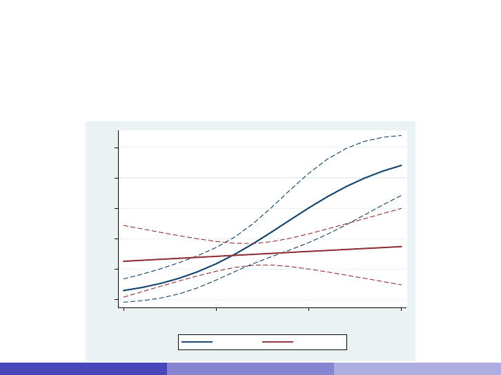
The at option
. quietly logit foreign mpg
. quietly eststo bivariate: margins, at(mpg=(10(2)40)) post
. quietly logit foreign mpg turn price
. quietly eststo multivariate: margins, at(mpg=(10(2)40)) post
. coefplot bivariate multivariate, at ytitle(Pr(foreign=1)) xtitle(Miles per Gallon) ///
¿ recast(line) lwidth(*2) ciopts(recast(rline) lpattern(dash))
0 .2 .4 .6 .8 1
Pr(foreign=1)
10 20 30 40
Miles per Gallon
bivariate multivariate
Ben Jann (University of Bern) Plotting Estimates Hamburg, 13.6.2014 44


StGBBetmGAuG
Total
Männer
Frauen
Total
Männer
Frauen
Total
Männer
Frauen
0 2 4 6 8 10 12 14 16 18 20 22 24 26
Beschuldigtenbelastungsrate (pro 1000 Einwohner)
Schweizer
In der Schweiz geboren (Niedergelassene)
Im Ausland geboren (Niedergelassene)
Besitz/
Sicherstellung
Konsum
Anbau/Herstellung,
Handel, Schmuggel
Europa
Afrika
Amerika
Asien
Europa
Afrika
Amerika
Asien
Europa
Afrika
Amerika
Asien
0 5 10 15 20 25
BBR (pro 1000 Einwohner)
0 .5 1 1.5 2 2.5 3
BBR (pro 1000 Einwohner)
Männer Frauen
18
20
27
9
13
15
3
1
10
3
4
8
2
-0
3
2
10
4
6
-3
7
1
5
-2
2
copying from
other
students in
exam
using crib
notes in exam
taking drugs
to enhance
exam
performance
including
plagiarism in
paper
handing in
someone
else's paper
DQ
RRT
CM
DQ
RRT
CM
DQ
RRT
CM
DQ
RRT
CM
DQ
RRT
CM
0 10 20 30 -5 0 5 10 15
Prevalence estimate in % Difference to DQ
-.02 0 .02 .04 .06 .08
Difference in survival rates
15 20 25 30 35 40 45 50 55 60 65 70 75 80
Age
-.02 0 .02 .04 .06 .08
Difference in survival rates
15 20 25 30 35 40 45 50 55 60 65 70 75 80
Age
-.02 0 .02 .04 .06 .08
Difference in survival rates
15 20 25 30 35 40 45 50 55 60 65 70 75 80
Age
controlling for country, sex, and birth cohort
controlling for country, sex, birth cohort,
childhood health, and cognitive ability at age 10
controlling for country, sex, birth cohort,
childhood health, cognitive ability at age 10,
and socio-economic life conditions at age 10
controlling for country, sex, birth cohort,
childhood health, cognitive ability at age 10,
socio-economic life conditions at age 10,
family situation at age 10, and periods of
financial hardship, stress, hunger, or happiness
Ben Jann (University of Bern) Plotting Estimates Hamburg, 13.6.2014 46

References I
Cleveland, William S. (1994). The Elements of Graphing Data (Revised
Edition). Murray Hill, NJ: AT&T Bell Laboratories.
Cleveland, William S., Robert McGill (1985). Graphical Perception and
Graphical Methods for Analyzing Scientific Data. Science 299(4716):
828-833.
Dice, Lee R., Harold J. Leraas (1936). A graphic method for comparing
several sets of measurements. Contributions from the Laboratory of
Vertebrate Genetics(3): 1-3.
Gallup, John Luke (2012). A new system for formatting estimation tables.
The Stata Journal 12(1): 3-28.
Harrell, Jr., Frank E. (2001). Regression Modeling Strategies. With
Applications to Linear Models, Logistic Regression, and Survival Analysis.
New York: Springer.
Ben Jann (University of Bern) Plotting Estimates Hamburg, 13.6.2014 47

References II
Jacoby, William G. (1997). Statistical Graphics for Univariate and Bivariate
Data. Thousand Oaks, CA: Sage.
Jann, Ben (2007). Making regression tables simplified. The Stata Journal
7(2): 227-244.
Kastellec, Jonathan P., Eduardo L. Leoni (2007). Using Graphs Instead of
Tables in Political Science. Perspectives on Politics 5(4): 755–771.
Lewandowsky, Stephan, Ian Spence (1989). The Perception of Statistical
Graphs. Sociological Methods & Research 18(2 & 3): 200-242.
Newson, Roger (2003). Confidence intervals and p-values for delivery to
the end user. The Stata Journal 3(3): 245-269.
Student (1927). Errors of Routine Analysis. Biometrika 19(1/2): 151-164.
Ben Jann (University of Bern) Plotting Estimates Hamburg, 13.6.2014 48
