LibreOffice Calc Conditional Formatting Guide

LibreOffice Calc

Conditional Formatting Guide

Table of contents
Preface................................................................................................................... 3
Introduction.......................................................................................................... 4
How to create, change and delete conditional formatting..............................5
1. Creating of conditional formatting.....................................................................................5
2. Changing of conditional formatting...................................................................................6
3. Deleting of existing conditional formatting......................................................................6
Several conditions for one cell range. Priority of conditions processing.......8
Creating own cell style for conditional formatting.........................................10
1. Dialog Cell style...................................................................................................................10
Category and types of conditional formatting................................................15
1. Category “All cells”...............................................................................................................15
2. Category “Cell value is”.......................................................................................................19
3. Category “Formula is”.........................................................................................................22
4. Category “Date”...................................................................................................................23
Copying of conditional formatting...................................................................26
2

1. Preface

This guide is intended for LibreOffice Calc users, who wants to use conditional for-

matting in their work.

All name of menu, toolbars, tooltips, dialogue, button and any other elements of

GUI are from LibreOffice Calc 6.0.3.

When I wrote this guide, I found some bugs in GUI and in execution of conditional

formatting in LibreOffice Calc 6.0.3. There are special reservations about it in the text.

It is requested that reader already knows how to work with computer and with

spreadsheets (LibreOffice Calc, MS Excel, Gnumeric or any one else), knows terms “Main

menu”, “Sheet”, “Cell”, “Range of cells”, “Address of cells”, etc.

Author of this guide is Roman Kuznetsov.

Very big thank you to Sophie Gautier for review of this guide and Mike Kaganski for

fixing some bugs in Conditional formatting I found when created this guide.

This guide is shared under Creative Commons Attribution ShareAlike version 4.0 li-

cense. Text of the license is reachable under this link:

https://creativecommons.org/licenses/by-sa/4.0/legalcode.

2. Introduction

Unfortunately, many users don’t use conditional formatting in their work. What is

conditional formatting and what it does??

At first, we define some terms:

Format cells – it is customizing of cell view. We can change the following options:

• Background color of cell;

• Showing, color and type of cell borders;

• Options of text view: vertical and horizontal text alignment in cell, rotation of text in

cell, text color, text effects, shadow of text, font and font style (bold, italic);

• Number format: Number, Percent, Currency, Date, Time, Scientific, Fraction, Bool-

ean value, Text.

Formatting of cells is used in order to highlight important information in spread-

sheet and to ease perception. Classic example is color highlighting of cells: green, yellow

and red. User shouldn’t think about meaning of numbers in cells, rows or columns. Color

indication of cells is more intuitive for people. Of course, you have to first understand

what means each type of condition and which result you want to achieve.

Cell style – it is a user defined set of options of cell customization, saved with

unique name for this document. LibreOffice Calc already has some pre-built cell styles,

that can be used for conditional formatting. User can create his own cell styles or change

existing styles.

Conditional formatting – it automatically applies cell style to cell or cell range

when user defined condition is performed. For example, you define automatically green

highlighting of cells, if cell value is between 80 and 100; or green highlight cell if there is

word “Russia” and red highlight if there is word “USA” in cell. If value in cell is changed,

then the formatting of cell will change too depending on the defined conditions.

Attention!

Make sure, that item Data►Calculate►AutoCalculate is active. It is need for condi-

tional formatting to work correctly.

So, by using conditional formatting, it allows user to forget about formatting of cells

when changing values in cells, LibreOffice Calc takes care of changing cell format itself.

Illustration 2.1: Formatting example

3. How to create, change and delete conditional formatting

3.1. Creating of conditional formatting

To create conditional formatting follow each of next steps:

1. Use sub-menu items Format►Conditional►(Condition; Color scale; Data bar;

icon set; Date).

2. Use Conditional widget on Formatting toolbar.

3. Use Add button in Manage Conditional Formatting dialog from Format► Condi-

tional► Manage menu

Whatever the used method, it opens Conditional Formatting for … dialog which al-

lows to customize conditional formatting.

To create conditions follow the next steps:

1. Think about the result you expect after using conditional formatting and which type

of condition you will use.

2. Select cell or cell range (during customizing of conditions it can be changed).

3. Open Conditional Formatting for … dialog using any method as shown above.

4. In Conditional Formatting for … dialog select for Condition 1 one of the available

category of conditions (All cells, Cell value is, Formula is or Date is).

5. Depending on the selected category set up options for conditional formatting. More

information will be in the following chapters.

6. If necessary, you can add several conditions for the same cell or cell range, click the

Add and repeat steps 4...6 as many times as you need.

7. Bottom part of the dialog has field Range, that allows to change the cell range of

your conditional formatting.

8. After finishing conditional customization, click the ОК button to close the Condi-

tional Formatting for … dialog.

9. If you opened Conditional Formatting for … dialog by using the Add button in

Manage Conditional Formatting dialog then click the OK button to close it too.

3.2. Changing of conditional formatting.

To change the existing conditional formatting follow next steps:

Illustration 3.1: Drop-down widget Conditional on Formatting toolbar

1. Select Format►Conditional►Manage in main menu to open Manage Conditional

Formatting dialog

2. Select the cell range, that you want to change.

3. Click the Edit button

4. Edit options of conditional formatting as written in items 4…9 in section «Creating of

conditional formatting» above.

Illustration 3.2: Conditional Formatting for... dialog

Illustration 3.3: Manage Conditional Formatting dialog

3.3. Deleting of existing conditional formatting.

To delete existing conditional formatting follow next steps:

1. Select Format►Conditional►Manage in main menu to open the Manage Condi-

tional Formatting dialogue

2. Select the cell range in the list where you want to delete conditional formatting.

3. Click the Delete button

4. Click the OK button to close the Manage Conditional Formatting dialog

4. Several conditions for one cell range.

Priority of conditions processing.

For one cell range you can create unlimited amount of conditions, but

Attention!

Very big amount of conditions in your spreadsheet or for one cell range can make work

with your document impossible. So don’t set up full rows (for example, 1:1) or full col-

umns (for example, A:A) for conditional formatting range, if you know, that your data

will be only in A1:B20 range.

Set up several conditions for one cell range is very simple:

Open Conditional Formatting for … dialog and click the Add button It adds a new

Condition 2, which can be customized the same as Condition 1. Add as many conditions as

you need.

Note, LibreOffice Calc processes conditions in list from top to bottom. Therefore po-

sition of conditions in the list is important.

Let’s see on the example below:

Set up for A1:A10 range three conditions from Cell value is category and select type

of condition Between:

For value in cell between 10 and 20 will select Good style (green);

For value in cell between 15 and 25 will select Bad style (red);

For value in cell between 20 and 30 will select Neutral style (yellow).

It is in this sequence from top to bottom.

Illustration 4.1: Example of priority of conditions for one range

Try enter number values in the cell A1….A10. If you type in cell any value from 15 to

20, then cell background will be green. But we have a second condition where cell back-

ground for range from 15 to 25 is red! Why do we have green color in cell? It is right, be-

cause condition with green background is higher than condition with red color in list of

conditions and first condition has more priority than second.

If you type in cell any value from 21 to 25, then cell background have red color. It’s

the same situation as above but for second and third conditions. Second condition has

more priority than third.

Also situation may happen where there are two (or more) intersecting cell ranges

with different conditional formatting. For example, there are cell range A1:A10 with own

conditions and A5:A15 with its own conditions. For cells in range А5:А10 first condition for-

matting will be processed that is first in list of ranges in Manage Conditional Formatting

dialog.

Attention!

Never make intersecting ranges of condition inside conditional formatting for one cell

range. And it’s not needed to make different conditional formatting for one cell range

or for intersecting cell ranges.

5. Creating own cell style for conditional formatting.

For some types of conditional formatting it is needed to set up cell style that will set

cell appearance if condition for the cell is met. LibreOffice Calc has some number built-in

cell styles with different cell views. But these styles are few or maybe you will need another

cell view. In this case you can create your own cell styles.

To create your own cell style select one from next variants:

1. Open the Sidebar and click the Style icon. Right click on the style named Default and

select the item New from context menu. It opens the Cell style dialog.

2. In the Conditional formatting for… dialog in Apple style drop-down list select the

item New style. It opens the same Cell style dialog.

3. Set up cell appearance as you need, then use the New style from selection icon in

top of the Style section on the Sidebar or use the menu item Styles ► New Style.

Enter a name for new style in the Create style dialog and click the OK button.

5.1. Dialog Cell style

Organizer tab.

On this tab, enter the name of the new style. Values in drop-down lists Inherit from

and Category are stay by default.

It’s better if the new style name is “selfspeaking”, for example “Red background with

Italic font” or “Bold violet font”.

Numbers tab.

On this tab you can set up options for numbers. There are several categories, each

of them have several formats.

Illustration 5.1: Cell style dialog. Organizer tab

Nothing change on this tab when you create cell style for conditional formatting.

Font tab.

On this tab you can select font, font style (bold, italic, regular), font size, language.

There is a preview area on the bottom part of the dialog.

Font effects tab.

There you’ll find opportunities available to customize font color, relief, on/off

shadow and outline. You can also set up overlining, striketrough and underlining.

Illustration 5.2: Cell style dialog. Numbers tab

Illustration 5.3: Cell style dialog. Font tab

Alignment tab.

You find text alignment and orientation parameters on this tab.

Borders tab.

Select cell borders, line style, width and color, padding and shadow style.

Illustration 5.4: Cell style dialog. Font e*ects tab

Illustration 5.5: Cell style dialog. Alignment tab

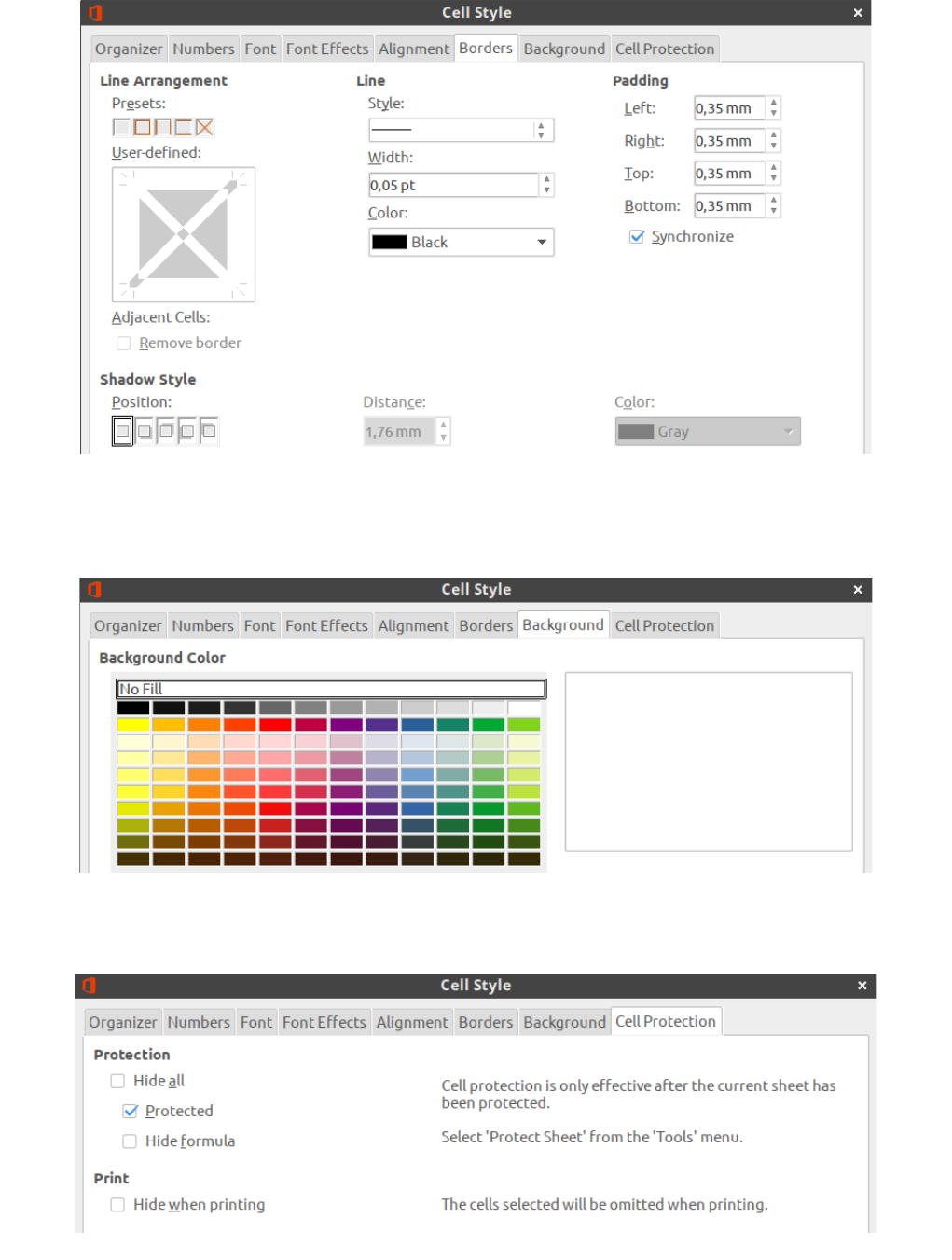
Background tab.

Select background color for cell.

Cell protection tab.

There are the options for cell protection on this tab.

When you create your own cell style for conditional formatting you should use only

options that change view of cell and do not touch others. Because target of conditional

formatting is to attract the user's attention or allow the user to quickly perceive informa-

Illustration 5.6: Cell style dialog. Borders tab

Illustration 5.7: Cell style dialog. Background tab

Illustration 5.8: Dialog Cell style. Cell protection tab

tion. Simplest way for this is by changing cell background color. Changing only of font view

is less often used

So all it needs is to set up style name, font options (font size, italic, bold, underline,

etc.) and cell background color.

After finishing to customize your new style click the OK button to save and close the

dialog.

Note

User’s cell styles will be save only in current spreadsheet file. To use your own styles for

conditional formatting in another file you should: copy cells with your own styles and

paste into another spreadsheet file. In the list of styles on the Sidebar your new styles

will be available and are available for use in the new file. Then you can delete inserted

data. Inserted styles will be available anyway.

6. Category and types of conditional formatting.

All available types of conditional formatting in LibreOffice Calc are divided in four

categories:

• All cells.

• Cell value is.

• Formula.

• Date.

Below we will consider in more detail all existing types of conditional formatting in

all categories.

6.1. Category “All cells”.

Types of conditional formatting from this category don’t work in one cell, it only

works for range from two and more cells. There are four types of conditional formatting in

this category.

Color scale (2 Entries).

This type of formatting analyzes number values in cell range and sets up color for

cell background depending on the value in the cell. User can select any color for minimum

value and maximum value.

By default it selected changing of color from minimum value to maximum value in

cell range. But you can select another option for extreme values from drop-down lists:

Min, Max, Percentile, Value, Percent, Formula.

Min – is in cell range it will automatically defines minimum value that will have the

start color.

Note

Item Min is in both drop-down lists. But this type of conditional formatting works fine if

you select Min only in left drop-down list, which defines the minimum value in range.

Max – in cell range will automatically defines maximum value that will have the fin-

ish color.

Note

Item Max is in both drop-down lists. But this type of conditional formatting works fine

if you select Max only in right drop-down list, which defines maximum value in range.

Illustration 6.1: All cells category. Color scale (2 Entries)

Percentile is a term from statistic. It works so: supposing we selected percentile

equaled 50. In our cell range Calc will sort ascending all values (doesn’t show it to user),

calculates the sequence number of cell by formula

=(quantity of cell in range)⋅50 % +1

and value in this cell became equal 50 percentile for our range, and all cells in range

with that value will have the selected color.

Value is numbering value selected by user in left drop-down list for minimum and in

right drop-down list for maximum. Cells with this value will have start or end color.

Percent is relative value of numeric value in cell in percent. Calculated by the for-

mula:

current value – minimum value in range

maximum value in range – minimum value inrange

Attention!

This Percent isn’t percent from maximum value in cell range in this case! You should

think about the expected result before using this variant!

Formula – type a formula under drop-down list. Result of formula will be use as

minimum (or maximum) value. Begin to type a formula by entering the “equal” sign. For

example, when you type in field formula =А1 then minimum (or maximum) value will be

equal to the value from cell A1. If value in cell A1 is changed, then conditional formatting

will be changed also.

Note

All cells less than minimum value from condition will have the same color as the one

selected for minimum value. And all cells more than maximum value from condition

will have the same color as the one selected for maximum value.

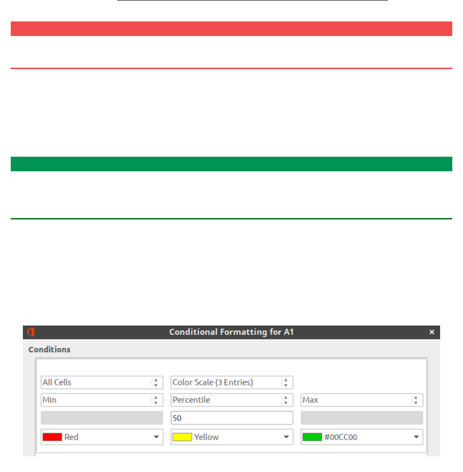
Color scale (3 Entries).

This type of conditional formatting analyzes numbering values in selected cell range

and set background color for it from two pairs of color: from minimum to intermediate

and from intermediate to maximum. So it uses three user defined colors. By default it

changes color by value in cell from minimum in range to maximum in range. Also it uses

additional mark – intermediate value equal 50 Percentile of range by default.

Intermediate value has its own color. You can select next option for extreme values

from drop-down lists: Min, Max, Percentile, Value, Percent, Formula. Those variants fully

coincides with variants for values in Color scale (2 Entries).

Illustration 6.2: All cells category. Color scale (2 Entries)

Data bar.

This type of conditional formatting analyzes number values in defined cell range

and shows in each cell a horizontal bar. Length of the bar depends from cell value. By de-

fault the filling of the bar is a gradient of blue color for positive values and red color for

negative values. By default there is a vertical axis with automatic position in cell that Calc

defines from cell values in range. It draws positive bar to right from vertical axis, negative

bar – to left.

There is additional options to customize data bars. Click the “More options...” but-

ton. It opens the “Data Bar” dialog, that allows to customize minimum and maximum val-

ues, bar colors for positive and negative values, fill type (gradient or color), position and

color of vertical axis, bar length and displays bar only without showing value in cells.

Icon set.

This type of conditional formatting analyzes number values in user defined cell

range and shows some icons in each cell. There are 22 icon sets for conditional formatting

in Calc.

Illustration 6.3: All cells category. Data bar

Illustration 6.4: Data bar dialog

There are icon sets of 3, 4 and 5 icons.

Select an icon set from the right drop-down list.

It is needed to set up border values for each icon in set (as «more or equal»). You

can select from drop-down lists next variants: Value, Percent, Percentile, Formula.

6.2. Category “Cell value is”.

Types of conditional formatting from this category works both for a single cell and

for a cell range. Most of the time, from types ask user to enter a value (or a formula, or a

link to cell) in the special field(s). Entered value will be compared with value in cell for the

process of conditional formatting. If condition is respected then cell will have the user de-

fined cell style. There are 24 types of condition in this category.

In the table below, you will find all types of conditions for this category and some

descriptions of how it works for each one:

Illustration 6.7: All cells category. Icon set

Illustration 6.5: Icon sets with 3 icons

Illustration 6.6: Icon sets with 4 and 5 icons

Type of condition Description

Equal to

The style is applied to the cell if value in cell is strictly equal to user defined

value in right field.

It works as for number values as for text in cells.

Note

If you want to check text in cell, then you should use quotes for

value in field, for example “Fire”.

Less than

The style is applied to the cell if value in cell is strictly less than user de-

fined value in right field.

It works only for number values in cells.

Greater than

The style is applied to the cell if value in cell is strictly greater than user de-

fined value in right field.

It works only for number values in cells.

Less than or equal to

The style is applied to the cell if value in cell is less than or equal to user

defined value in right field.

It works only for number values in cells.

Greater than or

equal to

The style is applied to the cell if value in cell is greater than or equal to user

defined value in right field.

It works only for number values in cells.

Not equal to

The style is applied to the cell if value in cell is strictly not equal to user de-

fined value in right field.

It works as for number values as for text in cells.

Note

If you want to check text in cell, then you should use quotes for

value in field, for example “Fire”.

Between

The style is applied to the cell if value in cell is between user defined values

in two right fields, including the values themselves.

It works only for number values in cells.

Not between

The style is applied to the cell if value in cell is not between user defined

values in two right fields, including the values themselves.

It works only for number values in cells.

Duplicate

The style is applied to the cell if value repeats in defined cell range two or

more time.

It works as for number values as for text in cells.

Not duplicate

The style is applied to the cell if value in cell is unique for defined cell

range.

It works as for number values as for text in cells.

Type of condition Description

Top 10 elements

Attention!

This name of type in GUI is wrong! Number of elements can be

set up any!

The style is applied to the cell if value in cell is in user defined number of

cells with maximum value for cell range.

It works only for number values in cells.

Bottom 10 elements

Attention!

This name of type in GUI is wrong! Number of elements can be

set up any!

The style is applied to the cell if value in cell is in user defined number of

cells with minimum value for cell range.

It works only for number values in cells.

Top 10 percent

Attention!

This name of type in GUI is wrong! It does not reflect the true

meaning of the condition!

The style is applied to the cell if value in cell is in user defined number of

cells (as a percentage of the total number of cells in the range) with maxi-

mum value for cell range.

It works only for number values in cells.

Bottom 10 percent

Attention!

This name of type in GUI is wrong! It does not reflect the true

meaning of the condition!

The style is applied to the cell if value in cell is in user defined number of

cells (as a percentage of the total number of cells in the range) with mini-

mum value for cell range.

It works only for number values in cells.

Above average

The style is applied to the cell if value in cell is strictly above average of all

values in cell range.

It works only for number values in cells.

Below average

The style is applied to the cell if value in cell is strictly below average of all

values in cell range.

It works only for number values in cells.

Above or equal aver-

age

The style is applied to the cell if value in cell is above or equal average of all

values in cell range.

It works only for number values in cells.

Below or equal aver-

age

The style is applied to the cell if value in cell is below or equal average of all

values in cell range.

It works only for number values in cells.

Error

The style is applied to the cell if value in cell is an internal error of Calc.

List of internal errors of Calc is on link.

Type of condition Description

No error

The style is applied to the cell if value in cell is not an internal error of Calc.

List of internal errors of Calc is on link.

Begins with

The style is applied to the cell if value in cell begins by user defined value in

right field.

Note

Recommended to set up condition as text (use quotes) even if

condition is a number. In this case Calc shows more correct re-

sult.

Ends with

The style is applied to the cell if value in cell ends by user defined value in

right field.

Note

Recommended to set up condition as text (use quotes) even if

condition is a number. In this case Calc shows more correct re-

sults.

Contains

The style is applied to the cell if value in cell contains user defined value in

right field.

Note

Recommended to set up condition as text (use quotes) even if

condition is a number. In this case Calc shows more correct re-

sults.

Not contains

The style is applied to the cell if value in cell doesn’t contain user defined

value in right field.

Note

Recommended to set up condition as text (use quotes) even if

condition is a number. In this case Calc shows more correct re-

sults.

6.3. Category “Formula is”.

In this category you enter a formula in special field. By using formulas you can real-

ize any condition from “Cell value is” category and any from your own condition. The style

is applied to the cell if value in cell corresponds to the result of the formula.

You can use all functions in your formula, that are present in Calc. For example, for

cell range (А1:А10) you can use this formula: А1=340, or А1<100, or А1<>”USA”, or

А1=”Contract is in work”. In this case cell A1 and next cells from range will be checked by

the corresponding result of the formula.

This category is one that allows to apply conditional formatting to cell or cell range

not matching with cell or cell range in condition.

In this case you should use the sign $ in cell address in the formula. In spread-

sheets, sign $ allows to fix cell or column number (or both) when you copy the formula in

to another cells.

Let’s see several examples:

Task: it is needed to highlight cell range B1:G1 by green color, if value in cell А1

equal to 100 (that is it needs to highlight row from the right of the checked cell).

Decision: enter a formula as $А1=100 and cell range as B1:G1. If you don’t write $

highlight only cell B1.

Task: it is needed to highlight cell range A2:A10 by green color, if value in cell А1

equal to 100 (that is it needs to highlight column below of the checked cell).

Decision: enter a formula as A$1=100 and cell range as А2:А10. If you don’t write

sign $ in formula, then Calc will not highlight all range А2:А10 by green color, but will high-

lights only cell A2.

Notice where the $ sign is in each case.

For cell range as B2:F20 in this case you should use the sign $ in formula as $A$1.

Attention!

There is an error in LibreOffice 6.0. You should select cell range or top left cell in future

conditional formatting range before opening the Condition formatting for… dialog (for

example, select cell B1 for cell range B1:G25). If you don’t do it, then conditional for-

matting may be work incorrect in some cases. If you see wrong conditional formatting,

then open the Manage Conditional Formatting dialogue and correct cell address to be

correct.

6.4. Category “Date”.

In this category you can set a condition for checking date in cells (number format in

cell should be “Date”). If the condition is met then cell will have user defined cell style. Date

in cell should be in full date format like in 23.09.2018 (DD.MM.YYYY) otherwise conditional

formatting will not work.

Note

Calc recalculate conditional formatting every time when you open the document.

Therefore, the result of conditional formatting today may differ from one month ear-

lier.

Here is a detail of the conditions:

Type of condition Description

Today

The style is applied to the cell if a date in cell is today.

Example of met condition:

Today is 20.08.2018 and date in cell is 20.08.2018

Yesterday

The style is applied to the cell if a date in cell is yesterday.

Example of met condition:

Today is 20.08.2018 and date in cell is 19.08.2018

Tomorrow

The style is applied to the cell if a date in cell is tomorrow.

Example of met condition:

Today is 20.08.2018 and date in cell is 21.08.2018

Type of condition Description

Last 7 days

The style is applied to the cell if a date in cell is any date from last 6 days or

today.

Example of met condition:

Today is 20.08.2018 and date in cell is any from 14.08.2018 to 20.08.2018

This week

The style is applied to the cell if a date in cell is any date from this week.

Attention!

In current version of LibreOffice Calc week begins from Sunday,

but not from Monday, as it is in England and USA. Please pay

attention to it when you will use this condition.

Example of met condition:

Today is 20.08.2018 (Monday on this week) and date in cell is any date from

19.08.2018 (Sunday on last week) to 25.08.2018 (Saturday on this week).

Last week

The style is applied to the cell if a date in cell is any date from last week.

Attention!

In current version of LibreOffice Calc week begins from Sunday,

but not from Monday, as it is in England and USA. Please pay

attention to it when you will use this condition.

Example of met condition:

Today is 20.08.2018 (Monday on this week) and date in cell is any date from

12.08.2018 (Sunday before last week) to 18.08.2018 (Saturday on last

week).

Next week

The style is applied to the cell if a date in cell is any date from next week.

Attention!

In current version of LibreOffice Calc week begins from Sunday,

but not from Monday, as it is in England and USA. Please pay

attention to it when you will use this condition.

Example of met condition:

Today is 20.08.2018 (Monday on this week) and date in cell is any date from

26.08.2018 (Sunday on this week) to 01.09.2018 (Saturday on next week).

This month

The style is applied to the cell if a date in cell is any date from this month.

Example of met condition:

Today is 20.08.2018 and date in cell is any date from 01.08.2018 to

31.08.2018.

Last month

The style is applied to the cell if a date in cell is any date from last month.

Example of met condition:

Today is 20.08.2018 and date in cell is any date from 01.07.2018 to

31.07.2018.

Next month

The style is applied to the cell if a date in cell is any date from next month.

Example of met condition:

Today is 20.08.2018 and date in cell is any date from 01.09.2018 to

30.09.2018.

Type of condition Description

This year

The style is applied to the cell if a date in cell is any date from this year.

Example of met condition:

Today is 20.08.2018 and date in cell is any date from 01.01.2018 to

31.12.2018.

Last year

The style is applied to the cell if a date in cell is any date from last year.

Example of met condition:

Today is 20.08.2018 and date in cell is any date from 01.01.2017 to

31.12.2017.

Next year

The style is applied to the cell if a date in cell is any date from next year.

Example of met condition:

Today is 20.08.2018 and date in cell is any date from 01.01.2019 to

31.12.2019.

7. Copying of conditional formatting.

We can set conditional formatting for one cell and then want to copy it to a cell

range. Or we have a cell range with conditional formatting and we want to increase the

cell range or copy conditional formatting to a new range, for example to another sheet.

How to copy conditional formatting or increase its cell range?

Variant №1.

Use Clone Formatting icon on toolbar.

Select the cell with conditional formatting. Double click on the icon. Then click on

the target cells in spreadsheet. When you finished copying hit Esc key on the keyboard.

Positive moment – it’s very fast and simple to make.

Negative moments:

– if there are many cells to be copied with conditional formatting, then it’s error

prone in addresses or ranges or you just get tired to click.

– LibreOffice 6.0 still has an error. When you copy conditional formatting to many

cells in dialogue “Manage Conditional Formatting” will create many different conditions

for each cell instead increasing existing cell range. In version 6.1 it will be fixed.

Variant №2.

Use dialogue “Paste Special”.

Select cell with conditional formatting. Copy it by any method (context menu, icon

on toolbar, etc.). Select the cell or cell range where you want to paste conditional format-

ting. Right click on selection and select item Paste Special > Paste Special… in context

menu. In “Paste Special” dialog deselect all options except Formats. Click the OK button.

Variant №3.

Use “Manage Conditional Formatting” dialog.

Select Format > Conditional > Manage menu A dialog box opens.

This dialog has a list of all cell ranges with conditional formatting on current sheet.

Select needed cell range. Click the Edit button at the bottom of the dialog. It opens the

Conditional Formatting dialog for <your cell range>.

There is a Range text field in the bottom part of the dialog. There you can set any

cell range. Use the standard address rule: enter, for example, А1:А50 or А1:В40, or several

ranges А1:А10;В5:В25, or cell range and different cells А1:А10;В4;С4:С15.

Attention!

Note, in the Range text field, there cannot be a space after ";" in address! Text box

should be highlighted with red color if there is an error in the address.