
Renewed for the Future: Renewable and Non-Renewable Energy
Sources and Their Costs
Jacob Nelson
The University of Akron
Department of Economics
Senior Project
Spring 2021

2
Abstract:
Renewable energy sources have come to the forefront of energy production policy
over the last twenty years. Studies of external and direct costs of both renewable
and nonrenewable energy sources have contributed to growing understandings of
ways in which these energy sources can be compared in a monetary context.
Using data from the U.S. Energy Information Administration (EIA) alongside
international data from the International Renewable Energy Agency (IRENA)
among other sources, we have developed forecasts for the future costs, both direct
and social, of each energy source as well as a difference-in-difference experiment
to determine potential effects of state-level energy policy changes on state level
energy prices. Forecasting is generally reliable as long as no major shocks to the
variables in question present themselves during the period being forecast. This
paper finds that renewable energy’s social and direct costs are both forecasted to
be lower than nonrenewable energy’s cost even while considering renewable
energy’s higher up-front costs. Additionally, statewide energy policy appears to
have no significant effect on renewable energy prices in the three years following
adoption, so further research with larger datasets is recommended.

3
Contents
Renewed for the Future: Renewable and Non-Renewable Energy Sources and Their Costs. .................. 1
I. Introduction ................................................................................................................................... 4
II. Literature Review .......................................................................................................................... 6
III. Data ......................................................................................................................................... 10
IV. Theory and Methodology ........................................................................................................ 14
V. Results ......................................................................................................................................... 19
VI. Conclusion .............................................................................................................................. 22
VII. References ............................................................................................................................... 23
Acknowledgements
I would like to thank Dr. Enami, Dr. Weinstein, and Dr. DeDad for their assistance provided for
this project. I would also like to thank the entire Department of Economics for inspiring my
classmates and me in our endeavors over our entire careers at The University of Akron.
4
I. Introduction
Energy markets across the globe have rapidly changed in the past twenty years in
response to new technology, problems, and production solutions. Renewable energy’s
technology and applications have advanced it to a position in which it can begin to compete with
traditional nonrenewable energy sources. Problems of pollution affecting public health, the
environment, and other resources have come to the forefront of national politics, and these new
renewable technologies offer a solution to the dangers of fossil fuels. Governments invest in and
look to these renewable energy sources to better serve their populations and maintain public
wellbeing in addition to ending reliance on the financially volatile fossil fuel economy.
There exists an alternative to renewable energies when emissions reductions are the goal.
One major alternative consists of a combination of the non-renewable sources with technologies
that reduce their negative environmental impact, such as carbon capture technology. This
alternative approach may be more cost-effective than adopting renewable energies in the near
future as it supplements already existing energy facilities creating a potentially cheaper solution
when compared to constructing entirely new renewable energy industries. Studies of the energy
market’s alternatives to renewables have focused on how to determine the cost of greenhouse gas
emissions reduction (Gillingham and Stock,2018; Kiuila and Rutherford, 2013), potential new
forms of carbon abatement (Lin and Ge, 2019), the economic and environmental impacts of
renewable energy sources (Varun, Bhat, and Prakash, 2009), and even a discussion of how much
fossil fuels would continue to be demanded in the future through a review of a worldwide
demand analysis (Pyper, 2018). However, there have been few publicly available analysis of if
prioritizing renewables would be an overall cheaper and more effective option for producing
energy in the near future, particularly in the next ten years.
5
Will it be more efficient to continue using fossil fuels with new carbon abatement
technologies in the US alongside renewables or will fossil fuels fall out of use due to abatement
technologies not making it as cost effective as renewables? Comparing the forecasted costs of
each of these energy sources while including the abatement cost of carbon emissions and the
public and environmental costs of fully utilizing renewable energy will allow policymakers to
see if it is more efficient for renewables to be used alongside fossil fuels for many years or if a
full switch to renewables should be done as soon as is technologically possible. Additionally, an
analysis of the relationship of costs to determine if and how renewable energy costs and fossil
fuel energy costs are related could prove useful in determining future actions. Finally, another
important question is: How have energy costs changed for US states that passed policy requiring
a certain percentage of energy production to be renewably produced? As the data is looked into
more deeply, these questions will be adjusted to determine which can be reasonably answered
with present day data.
Through the forecasting of key variables related to the costs of energy sources and an
application of these forecasted values to equations in order to craft estimates of per-kilowatt-hour
costs in the near future, comparisons between these two groups of energy sources are made.
Additionally, an analysis of differences in energy prices between states that have energy
portfolio requirements and those that do not is done to determine the short term effects of these
policy actions. The rest of this paper is organized as follows: a review of previous studies on
various facets of renewable energy followed by exploration of the data. From this foundation, a
review of economic theory informs the development of a methodology for creating a cost benefit
analysis alongside a difference-in-difference analysis. Finally, the results are organized into
graphs and conclusions are drawn from the models and projections created.
6
II. Literature Review
Previous cost benefit analyses (CBAs) have been conducted on both large and small
scales. The International Energy Agency (IEA) conducted a large-scale cost benefit analysis
throughout countries participating in their Renewable Energy Technology Deployment project
(RETD) to analyze technologies, costs, and externalities as well as more specific variables
relating to present day electrical systems. Given its comprehensive nature, this study provides a
general structure for how to conduct a CBA and data for variables such as the estimated external
costs of nonrenewable energy resources. For this study, costs are defined as long-run marginal
costs and benefits are excluded for simplicity’s sake. Some research has utilized consumer
willingness to pay to determine the benefits of renewable energy specifically, but no clear data is
available for this and the results of studies like this particularly Roe, et. al. (2001) are restricted
to the 1990s and early 2000s. The IEA analysis was in depth and attempted to discover which
forms of renewable energy have positive net benefits in comparison to more traditional sources
when externalities are not considered. The findings of this research point to hydro and wind
power having the lowest lifetime costs of generation with coal following close behind. Biomass
and Gas had roughly the same cost per megawatt hour, but biomass having much lower CO2
emissions. Additionally, analyses are done by the IEA that included externalities in total cost,
allowing an early comparison between renewable and nonrenewable sources despite limited data.
(IEA RETD, 2007).
Previous literature also discusses ways of determining costs and proper valuation on
external costs associated with energy production. The literature is not conclusive on the projected
costs and benefits of renewable energy, and no real benchmark numbers for energy costs are
available from the studies discussed. In Mathioulakis et. al. (2013), one such CBA was
7
undertaken in Greece and applied to “solar domestic hot water systems,” or water systems heated
by solar energy. The paper describes a utilization of net present value as one option in
determining the costs and utilizes an average of initial costs as well as maintenance costs and an
“expected lifetime” cost of their particular energy product (in this case, photovoltaic panels) to
develop the overall energy cost for their CBA (Mathioulakis et. al., 2013). The findings of this
study included the real energy savings by consumers who utilized these solar hot-water systems
and how these types of benefits can assist in supporting a more efficient power grid. Benefits
were developed in this model based largely around the “cost of saved electrical energy” from the
Athens network (Mathioulakis et. al., 2013). Despite the importance of net present value for cost-
benefit analyses as detailed in Mathiolakis et. al. (2013), the wide variation in estimates for
emissions costs creates a challenge in creating an NPV strategy for this study, so United States
Environmental Protection Agency (EPA) estimates will instead be used.
A major focus of renewable energy is the added benefit to consumers as can be revealed
in retail prices. Using retail prices to reveal these benefits have been done in past studies,
specifically hedonic housing studies. Roe et. al. (2001) conducted a survey of 1001 adults across
eight US cities and utilized a hedonic housing model controlling for premium prices of regional
“green energy” plans offered by electricity companies. The overall outcome of this research is a
linear regression model where each additional percent of renewable energy utilized increases
premiums by roughly $0.81, each percent of newly created renewable energy sources increases
these premiums by $6.21, and a “Green-e” certification for the energy provider provides a
$60.86 premium; this “Green-e” certification is representative of lower emissions. The authors
interpret these coefficients alongside their survey to conclude that the people surveyed most
likely value environmental benefits from both renewable energy and lower emissions, but lower
8
emissions are enough to convince consumers to pay premiums, even if renewable energy is not
championed (Roe et. al., 2001).
On the other hand, other researchers prefer to focus on more direct costs; the following
studies focus more closely on these direct costs. One study prefers to value renewable energy via
total life cycle benefits of each general type of plant (geothermal, wind, solar) available on
military bases and the total lifetime costs associated with these plants (McFaul and Rojas, 2012).
Although useful, the authors discuss the potential environmental benefits and costs associated
with these renewable sources but do not include them in their cost-benefit analysis. Some have
also attempted determining renewable energy cost through the abatement costs of nonrenewable
sources. Although not considered a true “valuation,” but instead a general “evaluation” by
Menegaki, abatement costs remain useful in developing, but not providing, effective estimates of
the cost of renewable energy (Menegaki, 2014). These abatement costs are utilized by the EPA
to develop the social costs utilized in our analysis. Finally, some researchers chose to value
renewable energy via determining the costs incurred to replace nonrenewable sources.
Replacement costs rest on the assumption that nonrenewable energy sources will be completely
replaced by renewables at some point in the future. In determining “sustainability” and
“economic welfare,” replacement cost theory is deemed sound by a critic of indices that utilize
replacement costs, but the same author champions a different, more complex, valuation method.
(Lawn, 2005). This is also in line with Menegaki’s approach, with an orientation around public
welfare being an essential part of cost-benefit analyses.
One of the simplest ways of estimating the production cost of electricity is to divide the
“annualized expenses of the [energy] system” by the “annual electricity generated by the
[energy] system” to gain a cent/kWh measure (Varun and Prakash, 2009). This may be simple
9
enough to utilize when comparing overall energy costs as renewables begin to represent a greater
percentage of overall energy usage. A report from the National Renewable Energy Laboratory
(NREL) also contributes in part to developing a lifetime cost of energy production facilities.
Through a study on the lifetime greenhouse gas (GHG) emissions by fuel source, it will be
possible to apply a cost to each fuel source utilized in a CBA to internalize this emissions
externality (NREL, 2013). Additionally, renewable energy sources reduction of GHG’s over
their lifetimes is an important benefit to discuss in implementing a holistic, welfare-oriented
CBA as described by Menegaki, and data on these benefits are presented in the NREL study. In
determining raw energy rates, another direct approach is available directly through data releases
from the US Department of Energy.
Externalities are another key part of costs discussed in the literature. Benefits, or reduced
costs as our study defines them, can be calculated through energy savings and environmental
wellbeing via emissions reductions (Mathioulakis et. al., 2013; Varun and Prakash, 2009). One
additional benefit that may be included is public health benefits, as emissions reductions also
influence this. One study estimated costs of abating CO
2
and willingness to pay for “reduced
mortality risk” to develop estimated benefits of renewable energy in each US region. This more
recent research provides useful numbers for estimating overall external costs associated with
health externalities (Buonocore et. al., 2019).
In addition to influencing public health and environmental factors, renewable energy
infrastructure (notably wind turbines) has also been assumed to create aesthetic externalities.
Hoen et. al.’s 2014 analysis Spatial Hedonic Analysis of the Effects of US Wind Energy Facilities
on Surrounding Property Values utilized a hedonic analysis in the US and found no evidence of
significant influence of wind energy’s visual or auditory status on nearby home prices, despite

10
previous studies with smaller sample sizes resulting in different conclusions. One such study
found that housing prices in Illinois were potentially lowered by 12-20% due to the presence of
visible wind turbines (Hinman, 2010). Although aesthetic externalities do not appear to influence
housing prices on a large scale, consumer preferences may not be fully explained in this analysis
or may be offset by some other feature of the region from which the data came. (Hoen et. al.,
2014)
III. Data
First, data is gathered from the US Energy Information Administration (EIA), the EIA’s
State Energy Data System (SEDS), the International Renewable Energy Agency (IRENA), and
the International Energy Agency (IEA). Data on electricity prices were unavailable in the time
period of 1984-1989 so they were left blank for that period of time. A large amount of SEDS
data also covers different variables associated with each energy source, so averages had to be
taken when they were not available directly within the data. Renewable energy costs before 2010
were not available, so forecasts were developed using only 2010-2019 data with zeroes excluded
from the fit procedure. Similarly, nonrenewable cost per kWh were not available after 2016, so it
had to be computed through available data on cost per short ton
1
of coal, cost per thousand cubic
feet of natural gas, and cost per barrel of crude oil each divided by the average kWh produced by
each of those metrics. Renewable energy as percent of total energy was developed through
dividing total renewable energy consumed by total primary energy consumed.
1
1 Short ton is equivalent to 2000 pounds and roughly 0.91 metric tons

11
The variables of interest as shown in Table 1 consist of energy production and
consumption metrics, price and cost data, and emissions data in determining the social cost of
each energy source as well as comparing reactions to state policy. The time series for these
variables are shown in Appendix A. First, energy production and consumption data are available
for certain sources, with most available data on fossil fuels being measured by production and
more renewable sources being calculated through consumption. These metrics are not equivalent,
due to losses while transporting, storing, and converting energy for use. Thus, it is imperative to
remember that the total energy consumed will be less than the total energy produced. However,
they will be assumed to be close enough for the comparison in this study. Both production and
consumption are assumed to increase over time with growing economies and growing
populations. Emissions data is largely available through the EPA, which determines social cost
of emissions (while including abatement costs in this estimate) for each unit of CO2 released into
the atmosphere and these emissions are expected to have a positive relationship with energy cost
due to environmental and health externalities. Energy cost is available through levelized cost
Table 1: Variables
Variable Name
Time Period
Source
Total Energy Expenditures
1980-2018
EIA
Total Energy Emissions
1980-2018
EIA
Renewable Energy Percent of
Total Energy
1980-2018
Created from two EIA
sources (Energy Production
and renewable Energy
Production)
Average Renewable Cost
2010-2018
IRENA
Average Nonrenewable Cost
1970-2018
Created from many EIA
sources (SEDS)
Average Retail Energy Price
1980-1983, 1989-2018
EIA
Figure 1: Variables Utilized to determine social costs.
Note: Total Expenditures, Emissions, and Renewable Energy Percent were removed from the analysis as ARIMA models were
adopted, replacing VAR model.
12
research, and much of the cost of renewable energy is calculated through these research releases
like those compiled by IRENA whereas fossil fuel cost is calculated through a combination of
production price determined by markets within the US and external costs associated with
reductions in CO2 emissions.
Each state also had data available in terms of prices and production costs from 1960 to
2018 through the EIA SEDS, allowing a difference-in-differences analysis to be attempted to
determine the change in energy cost as a result of renewable energy policy. Estimates of
abatement costs to develop a comparison between non-renewables and renewables are also
useful yet quite hard to determine. A plethora of studies have been done to determine abatement
costs in different industries, so applying one to the entire nation is not easy. In this general case
for comparison’s sake, an estimate of the social cost of CO2 as determined by the US
Environmental Protection Agency (EPA) is utilized. It must be noted that this estimate is not
perfect but considers the general social cost of each ton of CO2 rather than the cost needed to
abate CO2, allowing each industry’s (and even each plant’s) unique abatement cost to be ignored
in favor of a general cost summary. Abatement costs differ depending on industries and fuels,
but the cost of CO2 developed by the EPA takes into account these costs weighted by the amount
of energy produced by each nonrenewable energy source. Because of this method of estimation,
it is possible that, for example, despite the whole group of nonrenewable sources potentially
being more expensive than the whole renewable group, certain nonrenewable sources may be
less expensive than certain renewable sources.
Due to the nature of time series data, traditional descriptive statistics are not useful in
describing the data. Instead, augmented Dickey-Fuller tests assist in the determination of
stationarity in the data as that is required for the ARIMA model to function properly. In the

13
below figure (Figure 2), any p-values above 0.05 represent a significant probability of
stationarity in the data, so adjustments must be made in the ARIMA models to account for this.
The only non-stationary variable in this case is the cost of renewable energy (seen below as
“Renewable Cost”).
Figure 2: ADF Tests.
Note: Supported by clear visible trends in the graphs of the data
Additionally, autocorrelation functions like those below are utilized to ensure no autocorrelation
in the residuals of a series, which allows for more accurate forecasts. Autocorrelation is
essentially when the value of a time series is correlated with its own lags, which Each data series
is manipulated to ensure no autocorrelation within the residuals through differencing or
logarithmic transformation.

14
Figure 3: Autocorrelation Function of Total Emission's Residuals
Note: No lag being above or below confidence interval implies no significant autocorrelation in the series. See “Methodology”
for explanation of autocorrelation.
IV. Theory and Methodology
Theory
The most common costs discussed in theory and literature are the direct costs for
producing the energy. Both renewable and nonrenewable energy production requires set-up,
transportation, storage, and direct production costs. Further costs are incurred with the
production of energy through the traditional non-renewable methods such as coal, oil, and
natural gas. Gasses emitted from these sources such as CO
2
cause a plethora of health and
environmental problems that increase the costs of energy production on society (Buonocore et
al., 2019). Renewable energy technology aims to not only decrease the external costs of energy
to society but also the monetary costs associated with each kilowatt-hour of energy produced.
The combination of private costs and external costs create a cost to society for producing energy.
Renewable sources, such as solar and wind energy, have fewer negative effects on the health of
15
society and wellbeing of the environment, leading to their place as a possible replacement or
supplement to traditional fossil fuel energy production. On the other hand, non-renewable energy
sources, that may have a lower production costs, may be able to address their higher external
costs through technologies such as carbon abatement. The question then boils down to: Will
traditional energy sources with carbon abatement technology or renewable energy sources be
more socially efficient in producing energy in the future? Moreover, are renewable sources
economically feasible to compete with non-renewable energy on the national or international
stage without considering externalities?
Methodology
The foundation of the methodology lies in developing forecasts that can be used to create
useful estimated cost values. Each of the variables described in the data section will undergo
forecasting to obtain estimated values in the future. To develop overall costs of each method of
energy production, Autoregressive Integrated Moving Average (ARIMA) models are utilized to
forecast each cost to a specific point in the future and a summation of these costs gives us an
estimated total cost of that energy source per kilowatt-hour. Each specific variable has been
either sourced from government agencies and NGOs or created using available variables from
the former.
Autocorrelation Functions and Cross-correlation functions are utilized to ensure there is
little or no autocorrelation within individual variables or across different variables. As the time
series are annually reported, seasonal adjustment is unnecessary, but they are adjusted, if

16
necessary, to be stationarity. Differencing is also utilized to account for trends within the data
series, which makes the model an ARIMA model. Upon completion of fitting the model to the
data, autocorrelation functions are utilized to ensure no autocorrelation in the residuals of each
lag, which is essential for models such as these. Autocorrelation within the data from which the
forecast is created can lead to greater errors in our forecasts and generally make the forecast less
reliable. The overall process begins with a forecast of each aforementioned variable ten years
into the future using the fitted ARIMA models. As renewable energy has only come to the
forefront of production in the last twenty to thirty years, models based on the full dataset from
1980-2018, referred to later in the results as the “40 year data”, were supplemented with fits for
data from 2000-2018, referred to later as the “20 year data”. Each variable will have a forecast
generated using each length of data. The ARIMA(p,d,q) where p is the number of lags in the
model, d is the number of differences, and q is the order of moving average, can be described
with Equation 1:
Equation 1.
= +
y
+ +
y
e
e
+
where Φ is the AR parameter, ϴ is the MA parameter, and the number of differences is how
many times a previous lag of y
(also known as y
) is subtracted from y
, where y is our
variable of interest.
2
Each parameter is a single value applied by the forecast to develop the
model to be most accurate based on AIC values. Energy production costs are available from our
energy sources as per kwh measures. The external cost of emissions is calculated using estimates
from the EPA and applying it to average emissions per kWh of nonrenewable energy produced.
2
In this equation,
is simply the moving average error at lag t, which is the residual of the model to the actual
data.
17
Summing the per kilowatt-hour production cost and the per kilowatt-hour external costs results
in a per kilowatt-hour social cost of nonrenewable energy. On the other hand, renewable energy
cost results in negligible emissions and so the social cost equals the per kilowatt-hour production
cost. Variables for total energy expenditures, percentage of total energy produced by renewable
sources, and total emissions ended up not being utilized due to a change in the methodology
from a VAR model to multiple ARIMA models. These variables were still forecasted and are
present in Appendix B.
In addition to a forecast and a comparison of cost, this analysis will include state-to-state
comparisons to attempt to determine the effect of energy policy on retail energy price in that
state through a panel difference-in-differences analysis. This portion of the analysis will not be
utilizing forecasted values but will instead be a separate analysis utilizing the same data sources
between the years of 2004 and 2014. One additional data source, “State renewable portfolio
standards and goals” from the NCSL, is necessary to determine which states have which policies.
Marked differences in retail energy prices between two similar states who have different
makeups of energy production will be a sign that policy has an effect on cost in one way or
another. Energy cost differences between states can be influenced by demand for energy and fuel
costs, but nearby states with similar resources should be roughly comparable. T-Tests will be
utilized for the retail energy prices in these states to determine if their energy prices are before a
treatment (in this case, the treatment will be policy mandating increased utilization of renewable
energy) and then an analysis of the difference between an untreated state and a treated state will
estimate the effect of these policies on retail energy prices. Equation (2) represents the
difference-in-differences model in this analysis. The variables of interest are the left side variable
”EndPrice” which is made up of a three year average before and after the treatment is applied
18
for each state, the treatment variable “policy” which takes a value of “1” if the state establishes a
renewable energy portfolio policy between 2004 and 2014 and takes a value of “0” if no policy is
established or had been established before 2004, the time dummy variable “after” which uses a
value of “1” to identify the states in the post treatment period and “0” in the pre-treatment period,
and an interaction term between “policy” and “after.” The coefficient (
) of this interaction
term is the estimator for this diff-in-diff analysis. If this coefficient is deemed significant in the
final analysis, then we can say there is evidence of different retail prices after the treatment takes
place. The variable ε represents the error term of this model.
Equation 2.
=
+
+
+
(
)
+
(2)
19
V. Results
Due to changes in the energy landscape throughout the 1990s and early 2000s, only the
“20 year” data was utilized to develop forecasts and begin to determine social costs based on
different energy sources. Figures for each individual forecast and the individual orders of each
ARIMA model are in Appendix B below. These results point toward lower per-kWh social and
production costs for renewable energy sources going into the future. Figures 3 and 4 demonstrate
these differences with mean estimates alongside highs and lows with 95% confidence intervals.
The production cost and social cost graphs look quite similar because the estimates for the
emissions cost of nonrenewable energy is between one and two cents per kilowatt-hour (EPA).
External costs other than the cost of emissions were assumed to be negligible due to examples in
the literature, but there may be some external costs unaccounted for that could influence the
results. The results of the difference-in-differences point toward there being no significant
difference between retail energy prices in states that had renewable energy portfolio policies and
those that did not.

20
Figure 3: Forecasts of Social Costs and 95% Confidence Intervals
-$0.10
$0.00
$0.10
$0.20
$0.30
$0.40
$0.50
2019 2020 2021 2022 2023 2024 2025 2026 2027 2028
Cents Per Kilowatt-Hour
Forecasted Energy Social Cost per kWh
Renewable Energy Cost Nonrenewable Energy Cost

21
Figure 4: Forecasts of Direct Costs and 95% Confidence Intervals
-$0.10
-$0.05
$0.00
$0.05
$0.10
$0.15
$0.20
$0.25
$0.30
$0.35
$0.40
$0.45
2019 2020 2021 2022 2023 2024 2025 2026 2027 2028
Forecasted Energy Direct Cost per kWh
NON Nonrenewable Energy Cost REN Renewable Energy Cost
22
VI. Conclusion
The findings of this research can be summarized the social cost of renewable energy
being clearly lower than the social cost of nonrenewable energy. Additionally, we found no
significant differences in retail energy prices between states with and without renewable energy
portfolio policies. Renewable energy now appears to be a reasonable investment as the cost
continues to fall and the real reductions in external costs as a result of an increased use of
renewable energy sources further make the case for greater utilization of renewable energy. Even
when including the up-front costs of renewable energy facilities through the use of levelized cost
data, renewable energy provides lower direct per-kWh costs and vastly lower social per-kWh
costs. The lack of significant differences in retail prices between treated states and untreated
states in the three years following could imply the effects of these policies exist in the long term
rather than the short term or that incentives to energy producers to employ renewable energy
facilities would be more effective than policy requirements.
The models used for estimation could undoubtedly be improved. Future studies could
better define costs and benefits of energy sources and develop a more equal footing between the
energy sources. The lack of available production cost data for renewable energy sources and the
reliance on levelized cost research may have influenced the results in a biased manner and may
not represent the costs of renewable energy within the United States.

23
VII. References
Buonocore, J. J., Hughes, E. J., Michanowicz, D. R., Heo, J., Allen, J. G., & Williams, A.
(2019). Climate and health benefits of increasing renewable energy deployment in the
United States. Environmental Research Letters, 14(11), 114010. doi:10.1088/1748-
9326/ab49bc
Frequently asked Questions (FAQs) - U.S. Energy Information Administration (EIA).
Retrieved February 19, 2021, from https://www.eia.gov/tools/faqs/faq.php?id=19&t=3
Hinman, J. L. (2010). Wind Farm Proximity and Property Values: A Pooled Hedonic
Regression Analysis of Property Values in Central Illinois (Master's thesis, Illinois
State University, 2010). Pierre: South Dakota Public Utilities Commission.
doi:https://puc.sd.gov/commission/dockets/electric/2017/el17-055/exhibit4.pdf
Hoen, B., Brown, J., Jackson, T., Thayer, M., Wiser, R., & Cappers, P. Spatial Hedonic
Analysis of the Effects of US Wind Energy Facilities on Surrounding Property Values.
United States. https://doi.org/10.2172/1220223
International Renewable Energy Agency (IRENA). Renewable power generation costs in
2019. Retrieved February 21, 2021, from
https://www.irena.org/publications/2020/Jun/Renewable-Power-Costs-in-2019.
Lawn, P.A. An Assessment of the Valuation Methods Used to Calculate the Index of
Sustainable Economic Welfare (ISEW), Genuine Progress Indicator (GPI), and

24
Sustainable Net Benefit Index (SNBI). Environ Dev Sustain 7, 185–208 (2005).
https://doi.org/10.1007/s10668-005-7312-4
Mathioulakis, E., Panaras, G., & Belessiotis, V. (2013). Cost-benefit analysis of renewable
energy systems under uncertainties. 16th International Congress of Metrology.
doi:10.1051/metrology/201309002
McFaul, J., & Rojas, P. (2012). Comparative Cost-Benefit Analysis of Renewable Energy
Resource Trade Offs for Military Installations (Master's thesis, Naval Postgraduate
School, 2012). Fort Belvoir: DTIC. https://apps.dtic.mil/dtic/tr/fulltext/u2/a574363.pdf
Murshed, M., & Tanha, M. M. (2020). Oil price shocks and renewable ENERGY transition:
Empirical evidence from net Oil-importing South Asian economies. Energy, Ecology
and Environment. doi:10.1007/s40974-020-00168-0
National Renewable Energy Laboratory. (2013). Life Cycle Greenhouse Gas Emissions from
Electricity Generation [Fact Sheet]. NREL. https://doi.org/10.2172/1062479
Organization for Economic Co-operation and Development (OECD). Renewable Energy Costs
and Benefits for Society – Final Report. (2007). RECABS. Copenhagen: RETD ©
OECD/IEA.
Ricke, K., Drouet, L., Caldeira, K., & Tavoni, M. (2018). Country-level social cost of carbon.
Nature Climate Change, 8(10), 895-900. doi:10.1038/s41558-018-0282-y

25
Roe, B., Teisl, M. F., Levy, A., & Russell, M. (2001). US consumers’ willingness to pay for
green electricity. Energy Policy, 29(11), 917-925. doi:10.1016/s0301-4215(01)00006-4
U.S. Energy Information Administration (EIA). Retrieved February 19, 2021, from
https://www.eia.gov/.
U.S. Energy Information Administration - EIA – State Prices and Expenditures. (n.d.).
Retrieved February 19, 2021, from https://www.eia.gov/state/seds/seds-data-
complete.php?sid=US#PricesExpenditures.
U.S. Environmental Protection Agency (EPA) – Social Cost of Carbon. Retrieved February
19, 2021, from https://www.epa.gov/.
Varun, R., & Prakash, I. (2009, June 21). Energy, economics and environmental impacts of
renewable energy systems. Retrieved from
http://www.sciencedirect.com/science/article/pii/S136403210900094X.
26
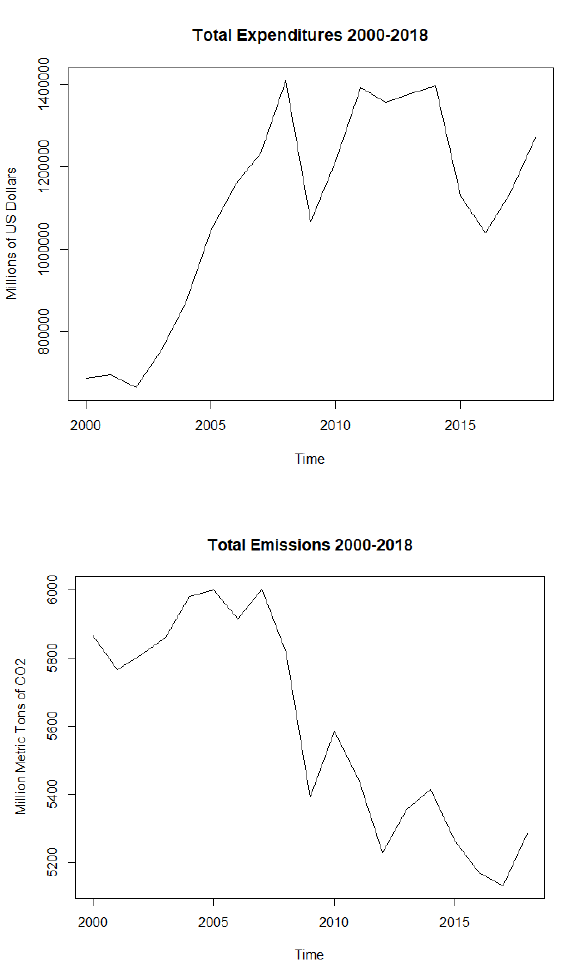
VIII. Appendix A
Time Series Graphs
The following figures are plotted data from IRENA (for renewable cost data) and the EIA
(all other variables) from 2000-2019.
Figure A1
Figure A2

27
Figure A3
Figure A4

28
Figure A5
Figure A6

29
IX. Appendix B
Forecast Graphs
The following figures are plots of the forecasted values for each variable. The bright blue
line is the mean estimated value with the area of gray representing a 95% confidence interval for
that forecast. Additionally, B7 contains the order of the ARIMA model for each variable.
Figure B1

30
Figure B2
Figure B3

31
Figure B4
Figure B5

32
Figure B6
Figure B7
Variable
ARIMA Order
Total Energy Expenditure
(1,0,0) (0,1,0)
Total Emissions
(1,0,0) (0,1,0)
Renewable Percent
(1,0,0) (0,1,0)
Renewable Cost
(1,0,0) (0,1,0)
Nonrenewable Cost
(0,0,0) (0,1,1)
Energy Retail Price
(2,0,0) (0,1,0)
X. Appendix C
R Code
#loading in datasets
library(readxl)
overall<-read_excel("C:/Users/joesc/Documents/SeniorYear/spring/Senior
Projec/doc3/data/mds.xlsx",
sheet="overall")

33
overall20<-read_excel("C:/Users/joesc/Documents/SeniorYear/spring/Senior
Projec/doc3/data/mds.xlsx",
sheet="overall20year")
library(forecast)
ts.totex<-ts(data=overall$TEE, start=1980, freq=1)
ts.totem<-ts(data=overall$TEM, start=1980, freq=1)
ts.renpct<-ts(data=overall$RPT, start=1980, freq=1)
ts.avgrencst<-ts(data=overall$REC, start=1980, freq=1)
ts.avgnoncst<-ts(data=overall$NEC, start=1980, freq=1)
ts.avgretprc<-ts(data=overall$REP, start=1980, freq=1)
ts.totex20<-ts(data=overall20$TEE, start=2000, freq=1)
ts.totem20<-ts(data=overall20$TEM, start=2000, freq=1)
ts.renpct20<-ts(data=overall20$RPT, start=2000, freq=1)
ts.avgrencst20<-ts(data=overall20$REC, start=2010, end=2018, freq=1)
ts.avgnoncst20<-ts(data=overall20$NEC, start=2000, freq=1)
ts.avgretprc20<-ts(data=overall20$REP, start=2000, freq=1)
#View Graphs
ts.plot(ts.totex20, main="Total Expenditures 2000-2018", ylab= "Millions of
US Dollars")
ts.plot(ts.totem20, main="Total Emissions 2000-2018", ylab="Million Metric
Tons of CO2")
ts.plot(ts.renpct20, main="Percent of Energy Produced by Renewable Sources in
the US 2000-2018", ylab="Percent")
ts.plot(ts.avgrencst20, main="Average Renewable Cost 2010-2019",
ylab="Dollars/KWH")
ts.plot(ts.avgnoncst20, main="Average Nonrenewable Cost 2000-2018",
ylab="Dollars/KWH")
ts.plot(ts.avgretprc20, main="Average US Energy Retail Price 2000-2018",
ylab="Dollars/KWH")
#making stationary
stl.totem<-(diff(log(ts.totem)))
stl.renpct<-(diff(log(ts.renpct)))
stl.avgrencst<-(diff(log(ts.avgrencst)))
stl.avgnoncst<-(diff(log(ts.avgnoncst)))
stl.avgretprc<-(diff(log(ts.avgretprc)))
acf(stl.totem, main="Autocorrelation Function Graph for Total
Emissions")
acf(stl.renpct)
acf(stl.avgrencst)
acf(stl.avgnoncst)
acf(stl.avgretprc)
ccf(stl.totem, stl.renpct)
ccf(stl.totem, stl.avgrencst)
ccf(stl.totem, stl.avgnoncst)
ccf(stl.totem, stl.avgretprc)
ccf(stl.renpct, stl.avgrencst)
ccf(stl.renpct, stl.avgnoncst)
ccf(stl.renpct, stl.avgretprc)
ccf(stl.avgrencst, stl.avgnoncst)
ccf(stl.avgrencst, stl.avgretprc)

34
ccf(stl.avgnoncst, stl.avgretprc)
stl.totem20<-(diff(ts.totem20))
acf(stl.totem20)
#correlations
library(ggpubr)
library(Hmisc)
library(corrplot)
coroverall<-cor(overall)
corrplot(coroverall)
#time series visual analysis
ts.plot(cbind(ts.totex, ts.renpct))
layout(1:2)
ts.plot(ts.avgrencst)
ts.plot(ts.renpct)
layout(1:2)
ts.plot(ts.totem, main="Total Emissions 1980-2018", ylab="Total Emissions
(Million Metric Tons CO2)")
abline(v=c(2008), col=c("blue"))
ts.plot(ts.renpct, main="Renewable Percent of Total Energy 1980-2018",
ylab="Renewable Percent of Total Energy (%)")
abline(v=c(2008), col=c("blue"))
#Time Series Dickey Fullers
library(tseries)
adf.test(ts.totex20)
adf.test(ts.totem20)
adf.test(ts.renpct20)
adf.test(ts.avgrencst20)
adf.test(ts.avgnoncst20)
adf.test(ts.avgretprc20)
#ARMA models
#ARMA 20 Year Data
fit.totex20<-auto.arima(ts.totex20, stepwise=FALSE, d=FALSE)
fc.totex20<-forecast(fit.totex20, h=10, level= c(95))
plot(fc.totex20, main="Forecast of Total Energy Expenditure",
ylab="US Dollars")
fit.totem20<-auto.arima(ts.totem20, stepwise=FALSE, d=FALSE)
fc.totem20<-forecast(fit.totem20, h=10, level= c(95))
plot(fc.totem20, main="Forecast of Total Emissions",
ylab="Metric Tons of CO2")
fit.renpct20<-auto.arima(ts.renpct20, stepwise=FALSE, d=FALSE)

35
fc.renpct20<-forecast(fit.renpct20, h=10, level= c(95))
plot(fc.renpct20, main="Forecast of Renewable Percent",
ylab="Percent of Energy from Renewable Sources")
fit.ren20<-auto.arima(ts.avgrencst20, stepwise=FALSE)
fc.ren20<-forecast(fit.ren20, h=10, level= c(95))
plot(fc.ren20, main="Forecast of Renewable Energy Cost",
ylab="USD per kWh")
fit.non20<-auto.arima(ts.avgnoncst20, stepwise=FALSE, d=FALSE)
fc.non20<-forecast(fit.non20, h=10, level= c(95))
plot(fc.non20, main="Forecast of Nonrenewable Energy Cost",
ylab="USD per kWh")
fit.ret20<-auto.arima(ts.avgretprc20, stepwise=FALSE, d=FALSE)
fc.ret20<-forecast(fit.ret20, h=10, level= c(95))
plot(fc.ret20, main="Forecast of Energy Retail Price", ylab="USD
per kWh")
#exporting forecasts
write.csv(rbind(fc.non20$mean, fc.ren20$mean, fc.renpct20$mean,
fc.ret20$mean, fc.totem20$mean, fc.totex20$mean),
file="C:/Users/joesc/Documents/SeniorYear/spring/Senior
Projec/forecasts.csv")
write.csv(rbind(fc.non20$upper, fc.ren20$upper, fc.renpct20$upper,
fc.ret20$upper, fc.totem20$upper, fc.totex20$upper),
file="C:/Users/joesc/Documents/SeniorYear/spring/Senior
Projec/forecastsupper.csv")
write.csv(rbind(fc.non20$lower, fc.ren20$lower, fc.renpct20$lower,
fc.ret20$lower, fc.totem20$lower, fc.totex20$lower),
file="C:/Users/joesc/Documents/SeniorYear/spring/Senior
Projec/forecastslower.csv")
#Difference in Difference
did<-
read_excel("C:/Users/joesc/Documents/SeniorYear/spring/Senior
Projec/DataForRevisedDiffInDiff.xlsx",
sheet="treatmenttest")
didreg <- lm(EndPrice ~ policy + after + int, data=did)
summary(didreg)
#No significant difference between states after treat
