Employment Hysteresis from the Great Recession

Employment Hysteresis

from the Great Recession

Danny Yagan

University of California, Berkeley, and National Bureau of Economic Research

This paper uses US local areas as a laboratory to test for long-term im-

pacts of the Great Recession. In administrative longitudinal data, I es-

timate that exposure to a 1 percentage point larger 2007–9 local un-

employment shock reduced 2015 working-age employment rates by

over 0.3 percentage points. Rescaled, this long-term recession impact

accounts for over half of the 2007–15 US age-adjusted employment de-

cline. Impacts were larger among older and lower-earning individuals

and typically involved a layoff but are present even in a mass-layoffs

sample. Disability insurance and out-migration yielded little income

replacement. These ﬁndings reveal that the Great Recession imposed

employment and income losses even after unemployment rates sig-

naled recovery.

I. Introduction

The US unemployment rate spiked from 5.0 percent to 10.0 percent over

the course of the Great Recession and then returned to 5.0 percent in

2015. However, the US employment rate (employment-population ratio)

I thank Patrick Kline, David Autor, David Card, Raj Chetty, Hilary Hoynes, Erik Hurst,

Lawrence Katz, Matthew Notowidigdo, Evan K. Rose, Jesse Rothstein, Emmanuel Saez, An-

toinette Schoar, Lawrence Summers, Till von Wachter, Owen Zidar, Eric Zwick, seminar

participants, and anonymous referees for helpful comments. Rose, Sam Karlin, and Carl

McPherson provided outstanding research assistance. I acknowledge ﬁnancial support from

the Laura and John Arnold Foundation and the Berkeley Institute for Research on Labor and

Employment. This work is a component of a larger project examining the effects of tax expen-

ditures on the budget deﬁcit and economic activity; all results based on tax data in this paper

are constructed using statistics in the updated SOI (Statistics of Income) Working Paper “The

Electronically published September 13, 2019

[ Journal of Political Economy, 2019, vol. 127, no. 5]

2505

This content downloaded from 136.152.029.121 on May 28, 2020 09:49:28 AM

All use subject to University of Chicago Press Terms and Conditions (http://www.journals.uchicago.edu/t-and-c).

did not exhibit similar recovery. Figure 1A shows that the employment

rate declined 3.6 percentage points between 2007 and 2015, as millions

of adults exited the labor force.

Population aging explains a minority of

the employment rate decline: weighting 2015 ages by the 2007 age distri-

bution reduces the decline to 2.0 percentage points, and the unadjusted

age 25–54 employment rate declined by 2.6 percentage points. The de-

cline was concentrated among the low skilled (Charles, Hurst, and Noto-

widigdo 2016). The decline’s persistence contrasts with employment rate

recovery after earlier recessions— leading history-based analyses such as

Fernald et al. (2017) to doubt the possibility of employment “hysteresis”:the

Great Recession having depressed long-term employment despite the

unemployment recovery.

This paper tests whether the Great Recession and its underlying sources

caused part of the 2007–15 age-adjusted decline in US employment or

whether that decline would have prevailed even in the absence of the

Great Recession. It is typically difﬁcult to test for long-term employment

impacts of recessions, for the simple reason that recession-independent

(“secular”) forces may also affect employment over long horizons (Ramey

2012). For example, the US employment rate rose by 2 percentage points

from the start of the 1981–82 recession to the late 1980s, as women con-

tinued to enter the labor force. In the context of the Great Recession, sec-

ular nationwide skill-biased shocks such as technical or trade changes

could have caused the entire 2007–15 employment decline, rather than

the recession.

I attempt to overcome this challenge by leveraging spatial variation in

Great Recession severity, along with data that minimize selection threats.

All US local areas by deﬁnition experienced the same secular nationwide

shocks, but some local areas experienced more severe Great Recession

shocks than other local areas. For example: Phoenix, Arizona—America’s

sixth-largest city—experienced a relatively large unemployment spike dur-

ing the Great Recession, while San Antonio, Texas—America’s seventh-

largest city—did not. A cross-area research design has the potential to dis-

tinguish recession impacts from secular nationwide shock impacts.

In the ﬁrst part of the paper, I show, using public state-year aggregates,

that a cross-area research design is indeed fertile ground for studying the

labor market consequences of the Great Recession. Deﬁning state-level

Variable deﬁnitions are standard and pertain to the age-16-and-over civilian noninsti-

tutional population.

This deﬁnition of hysterisis encompasses permanent impacts as well as transitory im-

pacts that last longer than elevated unemployment.

Home Mortgage Interest Deduction and Migratory Insurance over the Great Recession,” ap-

proved under Internal Revenue Service (IRS) contract TIRNO-12-P-00374 and presented at

the National Tax Association. The opinions expressed in this paper are those of the author

alone and do not necessarily reﬂect the views of the IRS or the US Treasury Department. Data

and programs are provided as supplementary material online.

2506 journal of political economy

This content downloaded from 136.152.029.121 on May 28, 2020 09:49:28 AM

All use subject to University of Chicago Press Terms and Conditions (http://www.journals.uchicago.edu/t-and-c).

shocks as 2007–9 employment growth forecast errors in an autoregressive

system (Blanchard and Katz 1992), I ﬁnd that 2015 employment rates re-

mained low in the US states that experienced relatively severe Great Re-

cession shocks—even though between-state differences in unemploy-

ment rates had returned to normal (and despite normal between-state

population reallocation). Hence, the cross-area patterns of employment,

unemployment, and labor force participation closely mirrored the aggre-

gate cross-time patterns of ﬁgure 1A. The persistent cross-area employ-

ment rate difference departs from the Blanchard-Katz ﬁnding of rapid re-

gional convergence.

The state-year evidence does not imply persistent employment impacts

of the Great Recession, because of two potential forms of cross-area com-

position bias: post-2007 sorting on labor supply and pre-2007 sorting on

human capital. First, severe Great Recession local shocks caused long-

term declines in local costs of living (Beraja, Hurst, and Ospina 2016),

which may have disproportionately attracted or retained those secularly

out of the workforce, such as the disabled and the retired (Notowidigdo

2011).

Even without such post-2007 sorting on labor supply, severe Great

Recession local shocks may have happened to hit areas with particularly

large preexisting concentrations of individuals affected by secular nation-

wide shocks. For example, the Great Recession disproportionately struck

local areas that had experienced housing booms (Mian and Suﬁ 2014) at-

tracting low- and middle-skill construction labor, and low- and middle-skill

laborers have been relatively adversely affected by secular nationwide

shocks in recent decades (e.g., Katz and Murphy 1992).

Under either type

of cross-area sorting, severe Great Recession local shocks may not have

caused local residents’ 2015 nonemployment.

I therefore turn for the second part of the paper to longitudinal linked

employer-employee data in order to control for prominent dimensions

of cross-area sorting. The longitudinal component allows one to measure

individuals’ employment over time regardless of whether and where in

the United States they migrated—directly controlling for post-2007 sort-

ing on labor supply. The linked employer-employee component allows

one to control for ﬁne interactions of age, 2006 earnings, and 2006 in-

dustry—proxies for pre-2007 human capital.

Speciﬁcally, I draw a 2 percent random sample of individuals from de-

identiﬁed federal income tax records spanning 1999–2015. The main

For example, “Warren Buffett’s Advice to a Boomer: Buy Your Sunbelt Retirement

Home Now” (Forbes, January 27, 2012; http://www.forbes.com/site s/janetnovack/2 012

/01/27/warren-buffetts-advice-to-a-boomer-buy-your-sunbelt-retirement-home-now/).

For example, “ You can’t change the carpenter into a nurse easily ...monetary policy

can’t retrain people” (Charles Plosser in “The Fed’s Easy Money Skeptic,” Wall Street Jour-

nal, February 12, 2011; http://www.wsj.com/articles/SB1000142405274870470930457612

4132413782592).

employment hysteresis from the great recession 2507

This content downloaded from 136.152.029.121 on May 28, 2020 09:49:28 AM

All use subject to University of Chicago Press Terms and Conditions (http://www.journals.uchicago.edu/t-and-c).

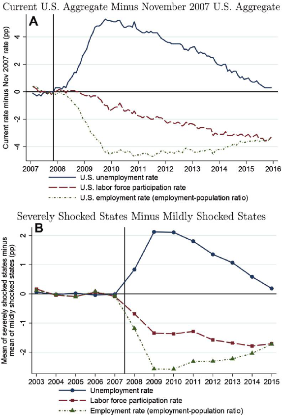
FIG.1.— Persistent employment rate declines after the Great Recession (pp: percentage

points). A, Data are from ofﬁcial seasonally adjusted BLS US labor force statistics from Jan-

uary 2007 through December 2015. The data are monthly and refer to the adult (161) ci-

vilian noninstitutional population. The vertical line denotes November 2007, the last

month before the Great Recession. For each outcome and month, the graph plots the cur-

rent value minus the November 2007 value, so that each data point in these series denotes a

percentage point change relative to November 2007. See online ﬁgure A.1 for age-adjusted

versions and versions restricted to 25–54-year-olds. B, US states are divided into severely

(below-median) and mildly (above-median) shocked states, based on 2007–9 state-level

employment growth forecast errors in the autoregressive system of Blanchard and Katz

This content downloaded from 136.152.029.121 on May 28, 2020 09:49:28 AM

All use subject to University of Chicago Press Terms and Conditions (http://www.journals.uchicago.edu/t-and-c).

outcome of interest is employment at any point in 2015, equal to an indi-

cator for whether the individual had any W-2 earnings or any 1099-MISC

independent contractor earnings in 2015. The main sample is restricted

to those aged 30–49 (“working age”) in 2007 in order to conﬁne the 1999–

2015 employment analysis to those between typical schooling and retire-

ment ages, and it is restricted to American citizens in order to minimize

unobserved employment in foreign countries. The analysis allows for

within-state variation by using the local-area concept of the commuting

zone (CZ): 722 county groupings that approximate local labor markets

and are similar to metropolitan statistical areas (MSAs) but span the en-

tire continental United States. I use the universe of information returns

to assign individuals to their January 2007 CZ. Each individual’s Great Re-

cession local shock equals the percentage point change in her 2007 CZ’s

unemployment rate between 2007 and 2009 as recorded in the Bureau

of Labor Statistics (BLS) Local Area Unemployment Statistics (LAUS).

I obtain 2006 four-digit North American Industry Classiﬁcation System

(NAICS) industry codes for half of 2006 W-2 earners by linking W-2s to

employers’ tax returns.

I ﬁnd that, conditional on 2006 age-earnings-industr y ﬁxed effects, a

1 percentage point higher Great Recession local shock caused the aver-

age working-age American to be 0.39 percentage points less likely to be

employed in 2015. The estimate is very statistically signiﬁcant, approxi-

mately linear in shock intensity, robust across numerous speciﬁcations,

and large: those living in 2007 in largest-shock-quintile CZs were 1.7 per-

centage points less likely to be employed in 2015 than initially similar in-

dividuals living in 2007 in smallest-shock-quintile CZs. Placebo tests indi-

cate no relative downward employment trend in severely shocked areas

before the recession, corroborating identiﬁcation. Controlling for 2015

local unemployment rates suggests that the incremental 2015 nonem-

ployment took the form of labor force exit rather than long-term unem-

ployment. I similarly ﬁnd impacts on 2015 wage and contractor earnings:

23.6 percent (2$997) of the individual’s preperiod earnings for every

1 percentage point higher shock.

One could be concerned that the foregoing within-industry analysis

fails to sufﬁciently control for pre-2007 sorting on human capital, as jobs

and therefore skill types in some industries are geographically differenti-

ated. Thus, as a novel robustness check, I approximate a within-job anal-

ysis, using a sample of 2006 workers at retail chain ﬁrms such as Walmart

(1992) estimated on 1976–2007 BLS LAUS state-year labor force statistics. For each out-

come and year, the graph uses LAUS to plot the unweighted mean in severely shocked

states, minus the same mean in mildly shocked states. Each series is demeaned relative to

its pre-2008 mean. See online appendixes A and B for more details.

employment hysteresis from the great recession 2509

This content downloaded from 136.152.029.121 on May 28, 2020 09:49:28 AM

All use subject to University of Chicago Press Terms and Conditions (http://www.journals.uchicago.edu/t-and-c).

and Safeway that employ workers with similar skills to perform similar

tasks at similar salaries in many different local areas. Adding ﬁrm ﬁxed ef-

fects in the retail sample attenuates the retail-sample employment effect

by 0.05 percentage points, or one-half of one standard error, to 20.36 per-

centage points, similar to the main estimate of 20.39 percentage points.

Certain comparisons suggest that the true average employment impact

could be closer to 20.30 percentage points per percentage point unem-

ployment rate shock. Naive extrapolation of the 20.30-for-1 and 20.39-

for-1 magnitudes would explain 58–76 percent of the US 2007–15 working-

age annual employment rate decline as a long-term impact of the Great

Recession. The actual implied aggregate impact depends on general equi-

librium ampliﬁcation or dampening.

The recession’s impacts were highly uneven within local areas. The em-

ployment and earnings impacts were most negative for older individuals

and those with low2006 earnings. The latter pattern indicates thatthe Great

Recession induced a long-term increase in employment and earnings in-

equality across skill levels, not merely within skill levels across space. Im-

pacts do not appear smaller among mobile subgroups such as renters or

the childless.

Adjustment via migration and social insurance appears highly incom-

plete in replacing lost income. I ﬁnd no statistically signiﬁcant impact of

Great Recession local shocks on out-migration from one’s 2007 CZ, and

earnings in other CZs did not replace any lost 2015 earnings relative to

those exposed to smaller Great Recession local shocks. Great Recession

localshockscausedsigniﬁcantlyhigherunemploymentinsurance(UI)ben-

eﬁts 2008–10 before UI beneﬁts expired and insigniﬁcantly higher So-

cialSecurityDisabilityInsurance(SSDI)beneﬁtsinallyears. I estimate that

2015 SSDI replaced 2 percent of lost 2015 earnings, or up to 6 percent at

the 95 percent conﬁdence upper bound.

Finally, I ﬁnd that most of the 2015 incrementally nonemployed in se-

verely shocked areas had been laid off at some point during 2007–14 and

were nonemployed in the entire 2013–15 period. However, higher layoff

rates do not appear to explain the results, as the impacts hold within a

sample of laid-off individuals. In particular, I ﬁnd equally large impacts

when comparing workers who were displaced in a 2008–9 mass layoff.

Hence, interactions with area-level economic conditions appear key to any

full explanation of the long-term impacts—such as human capital decay

during extended nonemployment or persistently low local labor demand.

The paper’s ﬁndings constitute evidence of long-term employment im-

pacts of the Great Recession (cf. Fernald et al. 2017) and add to a large lit-

erature on the incidence of labor market shocks. Earlier work had found

long-term impacts on individuals’ earnings (Topel 1990; Jacobson, La-

Londe, and Sullivan 1993; Neal 1995; Kahn 2010; Davis and von Wachter

2011) and sometimes on local areas’ employment rates (Blanchard and

2510 journal of political economy

This content downloaded from 136.152.029.121 on May 28, 2020 09:49:28 AM

All use subject to University of Chicago Press Terms and Conditions (http://www.journals.uchicago.edu/t-and-c).

Katz [1992] vs. Black, Daniel, and Sanders [2002] and Autor and Duggan

[2003]) and individuals’ employment rates (Ruhm [1991] and Walker

[2013] vs. Autor et al. [2014] and Jarosch [2015]). I provide evidence of

long-term impacts of Great Recession local shocks on individuals’ employ-

ment rates, likely via labor force exit. This evidence reinforces the view of

Autor and Duggan and a large literature dating back at least to Bowen and

Finegan(1969) and Phelps(1972)that transitoryadverseaggregateshocks

can have persistent negative employment impacts even after unemploy-

ment recovers.

The rest of the paper is organized as follows. Section II uses state-year

data to show that cross-area employment patterns mirrored aggregate

cross-time employment patterns 2007–15. Section III details the empiri-

cal design and longitudinal linked employer-employee data. Section IV

estimates overall impacts. Section V estimates impact heterogeneity. Sec-

tion VI investigates adjustment margins. Section VII documents layoff

and nonemployment trajectories. Section VIII discusses candidate mech-

anisms. Section IX concludes the paper.

II. Local Labor Markets Mirrored the Aggregate

This paper uses cross-area variation in Great Recession severity to test

whether the recession and its underlying sources caused part of the

2007–15 decline in the US employment rate displayed in ﬁgure 1A. I be-

gin by testing whether ﬁgure 1A’s aggregate cross-time employment pat-

terns have been mirrored across US local areas: did the local areas that

experienced severe Great Recession shocks also experience persistent

declines in employment and participation rates but not unemployment

rates, relative to mildly shocked areas? If so, then local labor markets may

indeed serve as a fruitful laboratory for understanding sources of aggre-

gate employment patterns.

A large literature has studied local labor market dynamics after local

employment shocks. The canonical analysis of Blanchard and Katz (1992)

found, in state-year data for 1976–90, that when a state experiences an ad-

verse employment shock, its population falls relative to trend but its un-

employment, participation, and employment rates return to parity with

those of other states in 5–6 years. That is, local shocks leave local areas

smaller but no less employed. This conclusion has been replicated in Eu-

ropean data (Decressin and Fatas 1995) and in a longer US state-year time

series (Dao, Furceri, and Loungani 2017). However, other papers have

found long-term participation and employment impacts of local shocks:

Black et al. (2002), Autor and Duggan (2003), and Autor, Dorn, and Han-

son (2013) found long-term impacts of speciﬁc types of US local shocks

on local SSDI enrollment, participation, and/or employment rates.

Hence, the existing literature presents a mixed picture.

employment hysteresis from the great recession 2511

This content downloaded from 136.152.029.121 on May 28, 2020 09:49:28 AM

All use subject to University of Chicago Press Terms and Conditions (http://www.journals.uchicago.edu/t-and-c).

This section documents local labor market dynamics after Great Reces-

sion local employment shocks, with greater detail presented in online

appendixes B and C. For comparability to the broadest line of previous

work, I conduct this analysis at the state level and categorize states into

severely shocked states and mildly shocked states, using unforecasted

state-level changes in 2007–9 employment, derived from the autoregres-

sive system of Blanchard and Katz (1992). I estimate Blanchard and Katz’s

log-linear autoregressive system in state employment growth, state unem-

ployment rates, and state participation rates in LAUS data for 1976–2007.

The LAUS data are the annual BLS LAUS series of employment, popula-

tion, unemployment, and labor force participation counts in 1976–2015

for 51 states (the 50 states plus the District of Columbia). Annual counts

are calendar year averages across months. I then compute 2008 and 2009

employment growth forecast errors for each state—equal to each state’sac-

tual log employment growth minus the system’s prediction for that state—

and sum the tw o to obtain each state’s 2007–9 employment shock. Ro ughly

speaking, each state’s shock equals the state’s 2007–9 log employment

change minus the state’s long-run trend. Then, for expositional simplicity,

I group the 26 states with the most-negative shocks (e.g., Arizona) into the

severely shocked category and the remaining states (e.g., Texas) into the

mildly shocked category.

Figure 1B displays the 2003–15 time series of unemployment, partici-

pation, and employment rate differences between severely shocked states

and mildly shocked states. For each outcome and year, the graph plots the

unweighted mean among severely shocked states minus the unweighted

mean among mildly shocked states (the graph looks nearly identical

weighting by population). Within each series, I subtract the mean pre-

2008 severe-minus-mild difference from each data point, so each plotted

series has a mean of zero before 2008.

The ﬁgure shows that the unemployment rate in severely shocked states

relative to that in mildly shocked states spiked in 2008, peaked in 2009–

10, and returned by 2015 to its mean prerecession severe-mild difference.

Yet the 2015 employment and participation rates in severely shocked

states remained 1.74 percentage points below the corresponding rates in

mildly shocked states, relative to the mean prerecession severe-mild dif-

ferences. The implied 2015 cross-area employment gap is large: 2.01 mil-

lion fewer adults were employed in severely shocked states than in mildly

shocked states, relative to full recovery to the prerecession severe-mild em-

ployment rate difference.

Hence, the cross-area (severe-minus-mild) patterns of unemployment,

participation, and employment of ﬁgure 1B do indeed broadly mirror

the aggregate cross-time (current-minus-2007) patterns of ﬁgure 1A.More-

over, in the same sense that the aggregate employment aftermath of the

Great Recession appears to contrast with the aftermath of the early-1980s

2512 journal of political economy

This content downloaded from 136.152.029.121 on May 28, 2020 09:49:28 AM

All use subject to University of Chicago Press Terms and Conditions (http://www.journals.uchicago.edu/t-and-c).

and early-1990s recessions, so too does the cross-area aftermath of the

Great Recession appear to contrast with the cross-area aftermath of those

earlier recessions. Figure 2A repeats the employment rate series of ﬁg-

ure 1B for the aftermath of the 1980s and 1990s recessions, treating the

early-1980s recessions as a single recession. The ﬁgure shows that cross-

state employment rates fully converged 4 years after the early-1990s reces-

sion and had converged by 1.65 percentage points (78 percent of the

t 5 0 divergence) 6 years after the early-1980s recession. Six-year conver-

gence aftertheGreatRecession wassmallerinbothabsoluteterms(0.85per-

centage points) and relative to the t 5 0 divergence (33 percent).

Blanchard and Katz(1992) suggest that the historical convergence mech-

anism is rapid population reallocation: a 21 percent state population

change relative to trend follows every 21 percent employment shock within

5–6 years.

Therefore,anatural possible explanationfor local employment

rate persistence after the Great Recession is that population reallocation

has slowed. Figure 2B investigates this possibility by plotting detrended

2007–14populationchanges—equalto eachstate’s2007–14percentchange

inpopulationminusthe2000–7percent changein thestate’spopulation—

versus the state’s 2007–9 employment shock. The graph shows that popu-

lation reallocation after the Great Recession was similar to the historical

benchmark: each 21 percent 2007–9 employment shock was on aver-

age accompanied by a 21.016 percent (robust standard error: 0.260) de-

trended population change.

Figure 2C shows the same conclusion when

the original Blanchard-Katz time range—1976–90, well before the recent

housing boom—is used to estimate state-speciﬁc population trends in the

Blanchard-Katz system. Population in severely shocked states fell in 2007–

15 relative to trend and relative to that of mildly shocked states, as much

as in the Blanchard-Katz benchmark.

To sum up, this section has found that aggregate 2007–15 cross-time

unemployment, participation, and employment rate patterns have been

mirrored in cross-area unemployment, participation, and employment

rate patterns over the same time period. Participation and employment

rates remained persistently low in the US states that experienced relatively

The unit elastic population response holds when reestimating the Blanchard and Katz

system on updated data for 1976–2015. The suggested causal chain is as follows: a state

(e.g., Michigan) experiences a one-time random-walk contraction in global consumer de-

mand for its locally produced traded good (e.g., cars), which induces a local labor demand

contraction and wage decline, which in turn induces a local labor supply (population) con-

traction, which then restores the original local wage and employment rate.

When not detrended, state population changes were largely uncorrelated with 2007–9

employment shocks, also shown in Mian and Suﬁ (2014) for the 2007–9 period only.

Blanchard and Katz (1992) ﬁnd adjustment via population changes relative to trend. Gross

(out-)migration rates have declined modestly since 1980 (Molloy, Smith, and Wozniak

2011), but gross ﬂows are still an order of magnitude larger than the net ﬂows (population

reallocations) predicted by history in response to 2007–9 shocks.

employment hysteresis from the great recession 2513

This content downloaded from 136.152.029.121 on May 28, 2020 09:49:28 AM

All use subject to University of Chicago Press Terms and Conditions (http://www.journals.uchicago.edu/t-and-c).

FIG.2.— Great Recession local adjustment in comparison to history. A, States are divided

into severely (below-median) and mildly (above-median) shocked states based on the sum

of 2008 and 2009 employment growth forecast errors, as described in ﬁgure 1B,repeating

the process for the early-1980s recessions (1980–82, treated as a single recession) and the

early-1990s (1990–91) recession. Then, for each recession and year relative to the reces-

sion, the graph plots the unweighted mean LAUS employment rate in severely shocked

states, minus the same mean in mildly shocked states. Each series is demeaned relative

to its prerecession mean. For comparability across recessions, year 0 denotes the last reces-

sion year (1982, 1991, or 2009), while year 21 denotes the last prerecession year (1979,

1989, or 2007); intervening years are not plotted. Online ﬁgure A.5 plots analogous graphs

for labor force participation, unemployment, employment growth, and population growth.

The post-2001-recession experience exhibited incomplete convergence before being inter-

rupted by positively correlated 2007–9 shocks (not shown). B, This graph uses LAUS data

to plot detrended 2007 –14 population changes—equal to each state’s 2007–14 percent

change in population minus its 2000–7 percent change in population—versus the state’s

2007–9 employment shock. Overlaid is the unweighted best-ﬁt line, with a slope of 1.016

(robust standard error of 0.260). C, The dotted lines plot Blanchard-Katz (1992) history-

based predictions (Pred.) for state-level responses to a 21 percent 2007–9 state-level em-

ployment shock, based on feeding the 1976–90-estimated Blanchard-Katz system a 2.41

percent employment shock followed by a 2.59 percent employment shock. The solid lines

plot mean actual (Act.) state-level responses based on reduced-form regressions of 2008–14

state-level outcomes on 2007–9 state-level shocks. See online appendix B for more details.

This content downloaded from 136.152.029.121 on May 28, 2020 09:49:28 AM

All use subject to University of Chicago Press Terms and Conditions (http://www.journals.uchicago.edu/t-and-c).

severe employment shocks 2007–9, even though unemployment rates con-

verged across space. Reduced population reallocation does not explain

the local persistence. The cross-area aftermath of the Great Recession de-

parts from the broad historical ﬁndings of Blanchard and Katz (1992),

but they accord with ﬁndings of Black et al. (2002), Autor and Duggan

(2003), and Autor et al. (2013) from speciﬁc contexts. I now turn to iden-

tifying whether Great Recession local shocks caused individuals to have

lower 2015 employment.

III. Isolating Impacts of Great Recession

Local Shocks

The previous section showed that local labor markets were microcosms

of aggregate employment patterns in 2007–15: 2015 employment rates

remained unusually low in US local areas that experienced an especially

severe 2007–9 employment shock. However, that cross-sectional fact does

not imply that individuals were nonemployed in 2015 because of where

they were living during the Great Recession, in light of two selection

threats. First, the disabled, retirees, and others secularly out of the labor

force may have disproportionately stayed in or moved to severely shocked

areas in order to enjoy low living costs while forgoing employment. Even

without selective migration on post-2007 labor supply, severely shocked

areas may have been disproportionately populated before the recession

by individuals who subsequently suffered large nationwide contractions

for their skill types, such as construction workers or routine laborers, that

would have occurred even in the absence of the recession. Under either

selection threat, the 2015 residents of severely shocked areas might be

nonemployed now regardless of geography.

This section speciﬁes my empirical strategy for using longitudinal

linked employer-employee data to isolate causal effects of Great Reces-

sion local shocks on individuals’ 2015 employment; 2015 is the most re-

cent year of data available. Additional details are listed in online appen-

dixes D and E, including design foundations in potential outcomes.

A. Empirical Design

I adopt an empirical design that closely follows earlier work using longi-

tudinal individual-level data to estimate long-term impacts of labor mar-

ket shocks (e.g., Jacobson et al. 1993; Davis and von Wachter 2011; Autor

et al. 2014). I estimate regressions of the form

i2015

5 bSHOCK

ci2007ðÞ

1 v

gi2006ðÞ

1 e

i2015

, (1)

where y denotes an employment or related outcome, i denotes an indi-

vidual, SHOCK

c(i2007)

is the Great Recession shock to the individual’s 2007

employment hysteresis from the great recession 2515

This content downloaded from 136.152.029.121 on May 28, 2020 09:49:28 AM

All use subject to University of Chicago Press Terms and Conditions (http://www.journals.uchicago.edu/t-and-c).

local area c, v

g(i2006)

denotes ﬁxed effects for groups g of individuals de-

ﬁned using individual pre-2007-determined characteristics, and e

i2015

a disturbance term. Here, b is the coefﬁcient of interest: the causal effect

on one’s 2015 outcomes of living in 2007 in a local area that experienced

a one-unit-larger Great Recession shock.

I interpret b as the causal effect of Great Recession local shocks and

their underlying sources, which are empirically indistinguishable,

and I

refer to this effect as the causal effect of Great Recession local shocks. Al-

ternative interpretations include b reﬂectin g differential prerecession trends

(e.g., a downward pre-2007 employment trend in severely shocked areas)

or independent correlated local shocks (e.g., post-2009 ﬂoods in severely

shocked areas). However, my interpretation of b is sensible because se-

verely shocked and mildly shocked areas exhibited relatively similar pre-

recession trends in the outcomes of interest (shown below in Sec. IV.A) and

because post-2010 unemployment rates converged monotonically across

severely shocked and mildly shocked areas. Moreover, adverse 2010–

15 industry-based shift-share shocks are not positively correlated with ad-

verse Great Recession local shocks.

As in earlier work, the identifying assumption is selection on observ-

ables: individuals were as good as randomly assigned across local areas

within groups g. Also as in earlier work, I aim to satisfy this assumption, us-

ing rich longitudinal data to deﬁne groups ﬁnely along dimensions (e.g.,

age, prerecession earnings, and prerecession industry) that could be cor-

related with both Great Recession local shocks and omitted secular na-

tionwide shocks, and to restrict attention to subsamples in which the iden-

tifying assumption is particularly likely to hold. I use event study graphs

to evaluate potentially confounding prerecession trends.

B. Samples

I implement the pape r’s empirical design by using selected deidentiﬁed

data from federal income tax records spanning 1999–2015. Iconstructthree

samples as follows. All three samples are balanced panels of individuals.

Main sample .—The main sample comprises a 2 percent random sample

from what I call the full sample. The full sample comprises all American

citizens aged 30–49 (“working age”) on January 1, 2007, who had not died

by December 31, 2015, and who had a valid payee ZIP code on at least one

information return that indicates continental US residence in January

For example, if the underlying source of Great Recession local shocks was persistent

local spending contractions (Mian, Rao, and Suﬁ 2013), then 2015 employment could

in principle be depressed because of layoffs during the Great Recession or because local

spending remained depressed through 2015, among other possibilities.

2516 journal of political economy

This content downloaded from 136.152.029.121 on May 28, 2020 09:49:28 AM

All use subject to University of Chicago Press Terms and Conditions (http://www.journals.uchicago.edu/t-and-c).

2007.

The age restriction conﬁnes the 1999–2015 employment analysis to

those older than schooling age and younger than retirement age. Birth,

death, andcitizenship data are drawn from Social Security Administration

(SSA) records housed alongside tax records.

Restricting attention to

those alive in 2015 excludes analysis of mortality effects, likely a conserva-

tive choice (Sullivan and von Wachter 2009). I describe geocoded informa-

tionreturnsin the next subsection.I randomly sampleindividuals fromthe

full sample by using the last two digits of the individual’s masked identiﬁca-

tion number, yielding a main sample comprising 1,357,974 individuals.

Retail chain sample.—The retail chain sample comprises individuals in

the full sample whose main employer in 2006 was a retail chain ﬁrm and

who lived outside the local area of the retail chain ﬁrm’s headquarters. It

is constructed as follows. For every individual in the full sample with a

2006 W-2 form, I attempt to link the masked employer identiﬁcation num-

ber (EIN) on the individual’s highest-paying 2006 W-2 to at least one busi-

ness return in the universe of business income tax returns 1999–2007.

I use the NAICS code on the business income tax return to restrict atten-

tion to workers whose 2006 ﬁrms operated in the two-digit NAICS retail

trade industries (44 or 45), for example, Walmart and Safeway.

I further

exclude employees living in 2007 in the CZ of their employer’s headquar-

ters, using the workers’ payee ZIP codes across their information returns

(see the next subsection) and the ﬁling ZIP code on business income tax

returns and mapping these ZIP codes to CZs (the local-area concept de-

ﬁned in the next subsection). Then, to identify CZs in which the 2006

ﬁrms operated, I further restrict thesample toﬁrms with at least 10 2006em-

ployees living in each of at least ﬁve CZs and then to the ﬁrms’ employees

living in 2007 in those CZs. This procedure yields a retail chain sample of

865,954 individuals at 524 retail ﬁrms.

In other contexts, “working age” sometimes refers to the age-15–65 population. My

sample lies within ages 15 and 65 in all years 1999–2015. I refer to the sample as working

age mainly to communicate that it omits individuals beyond normal retirement age.

Citizenship is recorded as of December 2016. Results are very similar when not condi-

tioned on citizenship status. Conditioning on citizenship reduces the possibility that 2007

residents are employed in other countries but appear nonemployed in US tax data.

Many ﬁrms’ workers cannot be linked to a business income tax return; see the next

subsection.

Accessed data lacked ﬁrm names. I do not know which speciﬁc ﬁrms survived the

sample restrictions. These example ﬁrms and their industry codes were found on Yahoo

Finance.

As in other US administrative data (e.g., the Census Bureau’s Longitudinal Employer

Household Dynamics; see Walker 2013), speciﬁc establishments of multiestablishment

ﬁrms are not directly identiﬁed in federal tax data. My process infers ﬁrms’ CZ-level oper-

ations from workers’ residential locations. The retail chain sample is smaller than the uni-

verse of retail chain workers for four main reasons: the age restriction, the de facto exclu-

sion of workers at independently owned franchises, mismatches between W-2 EIN and

business return EIN (see Sec. III.C.3 below), and removal of workers at ﬁrm headquarters.

employment hysteresis from the great recession 2517

This content downloaded from 136.152.029.121 on May 28, 2020 09:49:28 AM

All use subject to University of Chicago Press Terms and Conditions (http://www.journals.uchicago.edu/t-and-c).

Mass-layoffs sample.—The mass-layoffs sample comprises all individuals

in the full sample who separated from an employer during a mass-layoff

event in either 2008 or 2009, after having worked for the employer during

the prior three calendar years inclusive of the separation year. It is con-

structed as follows, closely adhering to the sampling frame of Davis and

von Wachter (2011), except that I deﬁne an employer as an EIN-CZ pair

rather than an EIN; an EIN may represent a ﬁrm or a division of a ﬁrm.

Using the universe of W-2s and linking W-2 payee (residential) ZIP codes

to CZs, I compute annual employment counts at the EIN-CZ level. For an

employer to qualify as having a mass-layoff event in year t ∈ f2008, 2009g,

the employer must satisfy the following conditions: it had at least 50 em-

ployees in t 2 1; employment contracted by between 30 and 99 percent

from t 2 1tot 1 1; employment in t 2 1 was no greater than 130 percent

of t 2 2 employment; and t 1 2 employment was less than 90 percent of

t 2 1employment.

The mass-layoffs sample comprises all 1,001,543 in-

dividuals in the full sample who received a W-2 with positive earnings from

a mass-layoff employer in years t 2 2 through year t but not in t 1 1.

C. Variable Deﬁnitions

I now deﬁne variables. Year always refers to calendar year. Variables are

available for 1999–2015.

1. Outcomes

Similar to usage by Davis and von Wachter (2011) and Autor et al. (2014),

employment in a given year is an indicator for whether an individual has

positive Form W-2 earnings or Form 1099-MISC independent contractor

earnings (both ﬁled mandatorily by the employer) in the year. Employ-

ment is thus a measure of having been employed at any time during the

year. Note that this annual employment measure differs from the conven-

tional point-in-time (survey reference week) measure used by the BLS. Al-

though not all self-employment is reported on 1099-MISCs, transition of

affectedworkerstoself-employmentlikelydoesnotexplaintheresults: Cur-

rentPopulationSurvey data indicatethatchanges in state self-employment

rates since 2007 were unrelated to changes in state formal employment

rates.

Earnings in a given year represents labor income and equals the sum of

an individual’s Form W-2 earnings and Form 1099-MISC independent

The 99 percent threshold protects against EIN changes yielding erroneous mass-layoff

events. The last two criteria exclude temporary employment ﬂuctuations. A ﬁrm that ini-

tially qualiﬁes as having mass-layoff events in both 2008 and 2009 is assigned a 2008 event

only.

2518 journal of political economy

This content downloaded from 136.152.029.121 on May 28, 2020 09:49:28 AM

All use subject to University of Chicago Press Terms and Conditions (http://www.journals.uchicago.edu/t-and-c).

contractor earnings. All dollar values are measured in 2015 dollars, ad-

justed for inﬂation using the headline consumer price index (CPI-U),

and are top-coded at $500,000 after inﬂation. DI receipt is an indicator for

whether the individual has positive SSDI income in the year as recorded

on Form 1099-SSA information returns ﬁled mandatorily by the SSA. SSDI

is the main US disability insurance program. UI receipt is an indicator for

whether the individual has positive UI beneﬁt income in the year as re-

corded on Form 1099-G information returns ﬁled mandatorily by state

governments.

2. CZ and Great Recession Local Shock

Allowing for within-state variation, an individual’s CZ is deﬁned as her res-

idential commuting zone, a local-area concept used in much recent work

(Dorn 2009; Autor et al. 2014; Chetty et al. 2014). CZs are collections of

adjacent counties, grouped by Tolbert and Sizer (1996) using commuting

patterns in the 1990 census to approximate local labor markets. I calcu-

late, based on the 2006–10 American Community Surveys, that 92.5 per-

cent of US workers live in the CZ in which they work. Urban CZs are sim-

ilar to MSAs, but whereas MSAs exclude rural areas, every spot in the

continental United States lies in exactly one of 722 CZs.

The 2007 CZ is the CZ corresponding to the payee (residential) ZIP

code that appears most frequently for the individual in 2006 among the

approximately 30 types of information returns (ﬁled mandatorily by insti-

tutions on behalf of an individual, including W-2s).

Information returns

are typically issued in January of the following year, so the ZIP code on an

individual’s 2006 information return typically refers to the individual’s

location as of January 2007. The 2015 CZ is deﬁned analogously to the

2007 CZ, except that if an individual lacks an information return in 2014,

I impute CZ using informationreturnZIPcode from the most recently pre-

ceding year in which the individual received an information return. The

2007 state denotes the state with most or all of the 2007 CZ’s population.

Each individual’s Great Recession local shock equals the percentage point

change in the individual’s 2007 CZ’s unemployment rate from 2007 to

2009. Annual CZunemploymentrates are computed by aggregating monthly

population-weighted county-level unemployment rates from the monthly

BLS LAUS series to the CZ-month level, then averaging evenly within CZ-

years across months. Measuring local shocks in unitsof the unemployment

Numerous activities trigger information returns, including formal and independent

contractor employment, SSA or UI beneﬁt receipt, mortgage interest payment, business

or other capital income, retirement account distribution, education and health savings ac-

count distribution, debt forgiveness, lottery winning, and college attendance. A compari-

son to external data suggests that 98.2 percent of the US population appeared on some

income tax or information return submitted to the IRS in 2003 (Mortenson et al. 2009).

employment hysteresis from the great recession 2519

This content downloaded from 136.152.029.121 on May 28, 2020 09:49:28 AM

All use subject to University of Chicago Press Terms and Conditions (http://www.journals.uchicago.edu/t-and-c).

rate change permits Section IV.D’s comparison to the aggregate shock,

which can be measured in the same units. Great Recession local shocks

are available on the author’s website, along with data that can be used to

approximate the paper’s main result using publicly available data, as dem-

onstrated in online appendix table 1.

3. Covariates

Age is deﬁned as of January 1 of the year, using date of birth from SSA

records housed alongside tax records. Female is an indicator for being re-

corded as female in SSA records. Following Autor et al. (2014), an indi-

vidual had high labor force attachment if she earned at least $10,382 in 2015

dollars—the compensation for 1,600 hours of work at the 2004 federal

minimum wage in 2015 dollars—in each of the four years 2003–6. An in-

dividual had no labor force attachment if she had zero earnings in any year

2003–6. All other individuals had low labor force attachment. The term

1040 ﬁler is an indicator for whether the individual appeared as either

a primary or secondary ﬁler on a Form 1040 tax return in tax year 2006.

Married is an indicator for whether the individual was either the primary

or secondary ﬁler on a married-ﬁling-jointly or married-ﬁling-separately

1040 return in tax year 2006. Number of kids equals the number of children

(zero, one, or two or more) living with the individual as recorded on the

individual’s 2006 Form 1040 if the individual was a 1040 ﬁler and zero oth-

erwise. Mortgage holder is an indicator for whether a Form 1098 informa-

tion return was issued on the individual’s behalf by a mortgage servicer in

2006.

Birth state is derived from SSA records and, for immigrants, equals

the state of naturalization.

The 2006 industry equals the four-digit NAICS industry code on the

business income tax return of an individual’s highest-paying 2006 Form

W-2, whenever a match can be made between the masked EIN on the W-2

and the masked EIN on the business income tax return. Four-digit NAICS

codes are quite narrow, distinguishing, for example, between restaurants

and bars. As displayed below in summary statistics and similar to recent

work (Mogstad, Lamadon, and Setzler 2017; Kline et al. 2018), almost half

of all W-2 earners could not be matched—likely because the employer is

a government entity (which does not ﬁle an income tax return, covering

15–20 percent of employment) or because the ﬁrm uses a different EIN

(e.g., a non-tax-ﬁling subsidiary) to pay workers from the one that appears

on the ﬁrm’s tax return. For the construction of ﬁxed effects, I assign in-

dividuals with a missing industry code to their own exclusive industry;

A mortgage servicer is required to ﬁle a Form 1098 on behalf of any individual from

whom the servicer receives at least $600 in mortgage interest on any one mortgage during

the calendar year.

2520 journal of political economy

This content downloaded from 136.152.029.121 on May 28, 2020 09:49:28 AM

All use subject to University of Chicago Press Terms and Conditions (http://www.journals.uchicago.edu/t-and-c).

I assign non-W-2-earning contractors to their own exclusive industry; and

I assign the nonemployed to their own exclusive industry. I show below

that results are nearly unchanged when the sample is restricted to the

nonemployed and those with a valid W-2 industry, for whom the correct

industry is universally observed.

The 2006 age-earnings-industry ﬁxed effects are interactions between age

(measured in one-year increments), 2006 industry, and 16 bins of the in-

dividual’s 2006 earnings (in 2015 dollars inﬂated by the CPI-U) from the

individual’s highest-paying employer.

The 2006 ﬁrm equals the masked

EIN on the individual’s highest-paying 2006 W-2. The 2006 age-earnings-

ﬁrm ﬁxed effects are constructed analogously to the 2006 age-earnings-

industry ﬁxed effects. Other controls are used only for robustness checks

and are deﬁned when used.

D. Summary Statistics

Table 1 reports summary statistics across the three samples. Of the main

sample, 79.1 percent were employed in 2015, with mean 2015 earnings

(including zeros and top-coded at $500,000) of $47,587; 6.2 percent re-

ceived SSDI income in 2015, and 25.6 percent received UI beneﬁt in-

come in at least one of the years 2007–14. The sample is 49.3 percent fe-

male; 62.4 percent had high labor force attachment in 2003–6. The

average 2006 age is 39.9 years. The retail chain sample is on average more

female, less attached to the labor force, and less likely to be married. The

mass-layoffs sample is on average less female, more attached to the labor

force, less likely to be married, and more likely to have worked in construc-

tion or manufacturing in 2006 than the main sample. Industry in the main

sample is observed for 51.1 percent of W-2 earners. The average Great

Recession local shock was a 2007–9 increase in the local unemployment rate

of 4.6 percentage points, with a standard deviation of 1.5 percentage points.

Each of the three samples comprises roughly one million individuals.

Figure 3 displays a heat map of Great Recession local shocks. Familiar

patterns are apparent, such as severe shocks in certain manufacturing ar-

eas and California’s Central Valley but not along California’s coast. Of the

variation in Great Recession local shocks, 30.0 percent is statistically ex-

plained by the house price–driven percent change in household net worth

in 2006–9 (Mian and Suﬁ 2009; correlation: 0.547). Recalling Section I’s

example, Phoenix—America’s sixth-largest city, shown in the medium-

dark-shaded CZ in the middle of Arizona—experienced a 77th percentile

The main result below is nearly identical when using Local CPI (consumer price in-

dex) 2—the more aggressive of the Moretti (2013) local price deﬂators—to locally deﬂate

2006 earnings before binning. Chosen to create roughly even-sized bins, the bin minimums

are $0, $2,000, $4,000, $6,000, $8,000, $10,000, $15,000, $20,000, $25,000, $30,000, $35,000,

$40,000, $45,000, $50,000, $75,000, and $100,000.

employment hysteresis from the great recession 2521

This content downloaded from 136.152.029.121 on May 28, 2020 09:49:28 AM

All use subject to University of Chicago Press Terms and Conditions (http://www.journals.uchicago.edu/t-and-c).

TABLE 1

Summary Statistics

Main Sample Retail Chain Sample Mass-Layoffs Sample

Mean

(1)

Standard Deviation

(2)

Mean

(3)

Standard Deviation

(4)

Mean

(5)

Standard Deviation

(6)

Outcomes (in 2015):

Employed (%) 79.1 40.7 81.8 38.5 84.1 36.5

Earnings (2015 $) 47,587 63,784 33,381 44,557 48,204 62,830

UI receipt sometime 2007–14 (%) 25.6 43.6 28.3 45.0 52.2 50.0

DI receipt (%) 6.2 24.2 6.9 25.3 6.0 23.8

Personal characteristics (in 2006, 2007):

Female (%) 49.3 50.0 60.8 48.8 44.5 49.7

Age (years) 39.9 5.7 39.2 5.8 39.7 5.7

Aged 30–34 (%) 22.2 41.5 27.0 44.4 23.8 42.6

Aged 35–39 (%) 24.5 43.0 25.0 43.3 25.0 43.3

Aged 40–44 (%) 26.0 43.9 24.3 42.9 25.5 43.6

Aged 45–49 (%) 27.3 44.6 23.6 42.5 25.7 43.7

Earnings (2015 $) 45,652 55,122 33,424 36,708 52,511 55,336

No labor force attachment (%) 22.7 41.9 15.1 35.8 10.0 29.9

Low labor force attachment (%) 14.9 35.6 24.3 42.9 16.4 37.1

High labor force attachment (%) 62.4 48.4 60.6 48.9 73.6 44.1

Married (%) 62.8 48.3 52.2 50.0 52.9 49.9

0 children (%) 36.2 48.0 41.8 49.3 40.6 49.1

1 children (%) 22.6 41.8 22.9 42.0 23.4 42.3

21 children (%) 41.2 49.2 35.4 47.8 36.0 48.0

2522

This content downloaded from 136.152.029.121 on May 28, 2020 09:49:28 AM

All use subject to University of Chicago Press Terms and Conditions (http://www.journals.uchicago.edu/t-and-c).

Mortgage holder (%) 38.3 48.6 25.9 43.8 38.4 48.6

Retail trade (NAICS 44,45; %) 5.2 22.3 100.0 .0 4.7 21.2

Construction/manufacturing (NAICS 23, 31–33; %) 11.9 32.4 .0 .0 17.7 38.2

Other observed industry (%) 25.9 43.8 .0 .0 34.9 47.7

Contractor (%) 4.2 20.1 .0 .0 .0 .0

Nonemployed (%) 11.5 31.9 .0 .0 .0 .0

Great Recession local shock (pp) 4.6 1.5 4.8 1.5 5.0 1.5

No. of individuals 1,357,974 865,954 1,001,543

No. of 2007 CZs 722 655 667

Note.—This table lists summary statistics for the paper’s three tax-data-based samples: the main sample (a 2 percent random sample), the retail chain

sample (all year-2006 nonheadquarters workers for identiﬁable retail chain ﬁrms), and the mass-layoffs sample (all workers who separated from a ﬁrm in a

2008 or 2009 mass layoff). All samples are restricted to American citizens aged 30–49 on January 1, 2007, who had not died by December 31, 2015 and who

had a continental United States ZIP code in January 2007. Earnings is the sum of W-2 wage earnings and 1099-MISC independent contractor earnings in the

calendar year, in 2015 dollars and top-coded at $500,000. “Employed” is an indicator for having positive earnings. “UI receipt sometime 2007–14” is an

indicator for having positive 1099-G unemployment insurance beneﬁt income at some point in 2007–14. “DI receipt” is an indicator for having positive

1099-SSA disability insurance income in the calendar year. Age is measured on January 1, 2007. Labor force attachment is high if the individual had, in

every year 2003–6, earnings above 1,600 hours times the federal minimum wage, zero if the individual was nonemployed in any year 2003–6, and low oth-

erwise. “Married” is an indicator for ﬁling a married-ﬁling-jointly or married-ﬁling-separately Form 1040 for tax year 2006. “Children” are dependent chil-

dren currently living with the individual as listed on the ﬁled 1040 form. A 1040 ﬁler is a primary or secondary ﬁler on a 1040 form for tax year 2006. Dis-

played marriage and number-of-children statistics are restricted to 1040 ﬁlers; in regressions controlling for marriage or number-of-children ﬁxed effects,

non-1040-ﬁlers are included as a separate group. “Mortgage holder” is an indicator for having positive mortgage payment listed on a Form 1098 in 2006

(mortgages held only in the name of a worker’s spouse or other third party are not included here). Industry categories are based on the NAICS code on the

business income tax return matched to the individual’ s highest-paying 2006 W-2 form. Nearly half of W-2 earners could not be matched, and individuals

who had only 1099-MISC independent contractor earnings are not matched; in ﬁxed-effect regressions, unmatched 2006 W-2 earners, contractors, and the

nonemployed are assigned to three separate industries. The 2007 CZ derives from the individual’s January 2007 residential ZIP code, as reﬂected most

commonly on her 2006 information returns. Great Recession local shock (pp: percentage points) equals the 2009 unemployment rate in the individual’s

2007 CZ minus the 2007 unemployment rate in that CZ as reported in the BLS LAUS.

2523

This content downloaded from 136.152.029.121 on May 28, 2020 09:49:28 AM

All use subject to University of Chicago Press Terms and Conditions (http://www.journals.uchicago.edu/t-and-c).

FIG.3.— Great Recession local shocks. This map depicts unweighted octiles (divisions by increments of 12.5 percentiles) of Great Recession local

shocks across commuting zones (CZs). CZs span the entire United States and are collections of counties that share strong commuting ties. Each

CZ’s shock equals the CZ’s 2009 LAUS unemployment rate minus the CZ’s 2007 LAUS unemployment rate. In the individual-level analysis, I assign

each individual to the Great Recession local shock of the individual’s January 2007 CZ.

This content downloaded from 136.152.029.121 on May 28, 2020 09:49:28 AM

All use subject to University of Chicago Press Terms and Conditions (http://www.journals.uchicago.edu/t-and-c).

shock (6.0 percentage points), while San Antonio—America’s seventh-

largest city, shown in the large, faintly shaded, landlocked CZ in the

middle-bottom of Texas—experienced a 7th percentile shock (2.6 per-

centage points). The empirical analysis compares the 2015 outcomes of

individuals who were living in 2007 in places like Phoenix to initially sim-

ilar individuals who were living in 2007 in places like San Antonio.

IV. Overall Impacts

This section presents the paper’s main result: the estimated effect on

2015 employment of Great Recession local shocks. I begin by presenting

the main regression estimate visually and in table form, followed by ro-

bustness and extrapolation exercises.

A. Preferred Estimates

Figure 4A plots the time series of estimated effects of Great Recession lo-

cal shocks on employment. Each year t’s data point equals

b from the fol-

lowing version of equation (1) estimated on the main sample:

5 bSHOCK

ci2007ðÞ

1 v

gi2006ðÞ

1 e

, (2)

where relative employment e

; EMPLOYED

2 ð1=8Þo

2006

s51999

EMPLOYED

is i’s change in mean binary employment status from pre-

recession years to year t,SHOCK

c(i2007)

denotes the Great Recession shock

to i’s 2007 CZ, and v

g(i2006)

denotes 2006 age-earnings-industry ﬁxed ef-

fects. Measuring employment outcomes relative to each individual’s pre-

recession mean transparently allows for baseline employment rate differ-

ences, similar to the relative cumulative earnings outcome of Autor et al.

(2014). The identifying assumption is that Great Recession local shocks

are as good as randomly assigned, conditional on age, initial earnings,

and initial industry. The sample and independent variable values are ﬁxed

across ﬁgure 4A’s annual regressions; only the outcome varies from year

to year. The 95 percent conﬁdence intervals are plotted in vertical lines

unadjusted for multiple hypotheses, based on standard errors clustered

by 2007 state.

The 2015 data point shows the paper’s main result: a 1 percentage

point higher Great Recession local shock (2007–9 spike in the CZ unem-

ployment rate) caused the average working-age American to be an esti-

mated 0.393 percentage points less likely to be employed in 2015. The

2015 impact of Great Recession local shocks is very signiﬁcantly different

from zero, with a t-statistic of 4.1.

Figure 4B supports the linear speciﬁcation of equation (2) by plotting

the underlying conditional expectation. It is constructed by regressing each

employment hysteresis from the great recession 2525

This content downloaded from 136.152.029.121 on May 28, 2020 09:49:28 AM

All use subject to University of Chicago Press Terms and Conditions (http://www.journals.uchicago.edu/t-and-c).

individual’sGreatRecessionlocalshock on theage-earnings-industryﬁxed

effects, computing residuals, adding the mean shock to the residuals, or-

dering and binning the residuals into 20 evenly sized bins, and plotting

mean 2015 relative employment within each bin versus the bin’s mean re-

sidual. The displayed nonparametric relationship between 2015 relative

employment and Great Recession local shocks is largely linear.

FIG.4.— Employment and earnings impacts of Great Recession local shocks. A, Regres-

sion estimates of the effect of Great Recession local shocks on relative employment, con-

trolling for 2006 age-earnings-industry ﬁxed effects in the main sample. Each year t’s out-

come is year t relative employment: the individual’s year t employment (indicator for any

employment in t) minus the individual’s mean 1999–2006 employment. The 95 percent con-

ﬁdence intervals are plotted around estimates, clustering on 2007 state. For reference, the

2015 data point (the paper’s main estimate) implies that a 1 percentage point higher Great

Recession local shock caused individuals to be 0.393 percentage points less likely to be em-

ployed in 2015. B, This graph nonparametricall y depicts the relationship underlying the main

estimate. It is produced by regressing Great Recession local shocks on 2006 age-earnings-

industry ﬁxed effects, computing residuals, adding back the mean shock level for interpre-

tation, and plotting means of 2015 relative employment within 20 equal-sized bins of the

shock residuals. Overlaid is the best-ﬁt line, whose slope equals 20.393. C, This graph rep-

licates A for the outcome of relative earnings: the individual’s year-t earnings minus the in-

dividual’s mean 1999–2006 earnings.

2526 journal of political economy

This content downloaded from 136.152.029.121 on May 28, 2020 09:49:28 AM

All use subject to University of Chicago Press Terms and Conditions (http://www.journals.uchicago.edu/t-and-c).

Returning to ﬁgure 4A, the prerecession time series of estimated ef-

fects constitute placebo tests supporting the identifying assumption that,

conditional on controls, Great Recession local shocks were as good as ran-

domly assigned. In particular, the 1999–2006 point estimates do not dis-

play a downwardpretrend that would suggest a negative 2015 point estimate

even in the absence of Great Recession local shocks. The graph makes

other statistics possible. For example, the 1999–2006 point estimates aver-

age zero by construction, but one could prefer to benchmark the 2015 es-

timate to a subset of prerecession estimates such as those for 1999–2001;

when subtracting the 1999–2001 mean estimate from the 2015 estimate,

one obtains the still-large effect of 20.316. When subtracting the 2004–

6 mean estimate, one obtains 20.507.

Table 2 displays coefﬁcient estimates from equation (2) in the main

sample under various speciﬁcations. Column 4 corresponds to ﬁgure 4A’s

2015 data point, my preferred estimate. Columns 1–3 replicate the analysis

with coarser ﬁxed effects and yield similar results, indicating relatively lit-

tle selection on the controlled dimensions among working-age Ameri-

cans. Column 5 displays ordered effect sizes by shock quintile, indicating,

for example, that living in 2007 in the most shocked quintile of CZs re-

sulted in the average individual being 1.75 percentage points less likely

to be employed in 2015 relative to living in 2007 in the least shocked quin-

tile. These effects are large, in that they are similar in magnitude to the

age-adjusted US employment rate decline 2007–15.

Full-year nonemployment indicates either long-term unemployment or

labor force nonparticipation (“exit”). Unemployment and participation

are not observed in tax data. To provide an indication of whether the non-

employment effects of Great Recession local shocks reﬂect labor force

exit, I test whether controlling for local unemployment persistence—

equal to the CZ’s 2015 unemployment rate minus its 2007 unemployment

rate—in the individual’s 2007 CZ (col. 6) or 2015 CZ (col. 7) attenuates

the main estimate. This test can be viewed as co nservative: controlling for

epsilon-higher unemployment persistence in relatively severely shocked

areas could fully attenuate the main estimate without that unemployment

persistence being able to explain it quantitatively. In practice, the controls

in columns 6 and 7 slightly and insigniﬁcantly attenuate the main estimate

from 20.393 to 20.366 and 20.364, respectively. This suggests that most

and possibly all of the 2015 nonemployment impact of Great Recession

local shocks took the form of labor force exit, consistent with cross-state

patterns in ﬁgure 1B.

Local unemployment rates converged throughout 2015. When only the July–

December period was used to deﬁne local unemployment persistence, the controls in

cols. 6 and 7 leave the estimate unchanged, at 20.392 and 20.393, respectively.

employment hysteresis from the great recession 2527

This content downloaded from 136.152.029.121 on May 28, 2020 09:49:28 AM

All use subject to University of Chicago Press Terms and Conditions (http://www.journals.uchicago.edu/t-and-c).

TABLE 2

2015 Impacts of Great Recession (GR) Local Shocks: Outcomes Relative to Pre-2007 Mean

N 5 1,357,974

A. 2015 Employment (pp)

(1) (2) (3) (4) (5) (6) (7)

GR local shock 2.412 2.425 2.417 2.393 2.366 2.364

(.112) (.112) (.099) (.097) (.089) (.089)

Most severely shocked quintile 21.746

(.471)

Fourth shock quintile 21.144

(.434)

Third shock quintile 2.793

(.356)

Second shock quintile 2.181

(.320)

Age FEs X

Age-earnings FEs X

Age-earnings-industry FEs XXXX

Unemployment persistence in 2007 CZ X

Unemployment persistence in 2015 CZ X

.00 .00 .01 .07 .07 .07 .07

Outcome mean 27.23 27.23 27.23 27.23 27.23 27.23 27.23

Absolute outcome mean 79.1 79.1 79.1 79.1 79.1 79.1 79.1

Standard deviation of GR local shocks 1.49 1.49 1.49 1.49 1.49 1.49 1.49

Interquartile range of GR local shocks 2.31 2.31 2.31 2.31 2.31 2.31 2.31

2528

This content downloaded from 136.152.029.121 on May 28, 2020 09:49:28 AM

All use subject to University of Chicago Press Terms and Conditions (http://www.journals.uchicago.edu/t-and-c).

B. Additional Outcomes and Controls

Cumulative Employment

2009–15 (pp)

Earnings in

2015 ($)

Cumulative Earnings

2009–15 ($)

Employed in 2015 (pp)

(8) (9) (10) (11) (12) (13)

GR local shock 22.700 2997 26,212 2.364 2.480 2.378

(.516) (168) (919) (.100) (.133) (.112)

Rust CZ  GR local shock .067 2.035

(.192) (.148)

Other CZ  GR local shock .094

(.250)

Age-earnings-industry FEs X X X X X X

Manufacturing share X

.07 .11 .13 .07 .07 .07

Outcome mean 240.5 6,249 27,646 27.23 27.23 27.23

Absolute outcome mean 563.9 47,587 317,011 79.1 79.1 79.1

Standard deviation of GR local shocks 1.49 1.49 1.49 1.49 1.49 1.49

Interquartile range of GR local shocks 2.31 2.31 2.31 2.31 2.31 2.31

Note.—All columns except col. 5 report coefﬁcient estimates of the effect of Great Recession local shocks on postrecession outcomes in the main sample.

Column 5 divides individuals into quintiles based on their Great Recession local shocks and reports coefﬁcients on indicators of shock quintiles, relative to the

least shocked quintile. Age ﬁxed effects (FEs) are birth year indicators. Earnings FEs are indicators for 16 bins in the individual’ s 2006 earnings. Industry FEs

are indicators for the individual’s 2006 four-digit NAICS industry. Local unemployment persistence equals the 2015 LAUS unemployment rate minus the 2007

LAUS unemployment rate in either the individual’s 2007 CZ or the individual’s 2015 CZ. The outcome in cols. 1–7 is 2015 relative employment: the individual’s

2015 employment (indicator for any employment in 2015) minus the individual’s mean 1999– 2006 employment. The col. 8 outcome equals the sum of the

individual’s 2009–15 employment minus seven times the individual’s mean 1999–2006 employment. The col. 9 outcome equals the individual’s 2015 earnings

minus the individual’s mean 1999–2006 earnings. The col. 10 outcome equals the sum of the individual’s 2009–15 earnings minus seven times the individual’s

mean 1999–2006 earnings. Column 11 controls for the 2000 manufacturing share of employment in the individual ’s 2007 CZ, computed in County Business

Patterns. Columns 11 and 12 control for indicators (not shown) and interactions of a Rust-CZ indicator and an Other-CZ indicator, based on the individual’s

2007 CZ. A Rust CZ is a CZ with an above-median manufacturing share; an Other CZ is a CZ with a below-median manufacturing share and an above median

2006–9 change in housing net worth from Mian and Suﬁ (2014). The absolute outcome mean equals the outcome mean before subtraction of the prerecession

mean. Standard errors (in parentheses) are clustered by 2007 state. For reference, col. 4 (the paper’s main speciﬁcation) indicates that a 1 percentage point

higher Great Recession local shock caused individuals to be 0.393 percentage points less likely to be employed in 2015.

2529

This content downloaded from 136.152.029.121 on May 28, 2020 09:49:28 AM

All use subject to University of Chicago Press Terms and Conditions (http://www.journals.uchicago.edu/t-and-c).

Figure 4C repeats ﬁgure 4A for the alternative outcome of relative

earnings: EARNINGS

2 ð1=8Þo

2006

s51999

EARNINGS

. Similar to ﬁgure 4A’s,

ﬁgure 4C’s coefﬁcient estimates exhibit no consistent trend in the prere-

cession period and then fall persistently after the recession. Table 2, col-

umn 9, presents the graph’s 2015 data point, which indicates that living

in 2007 in a CZ that experienced a 1 percentage point higher unemploy-

ment shock caused the average working-age American to earn 997 fewer

dollars in 2015.

Column 10 indicates that when cumulative relative earn-

ings o

2015

t52009

½EARNINGS

2 ð1=8Þo

2006

s51999

EARNINGS

 are considered, the

effect size cumulates to 2$6,212 over the 7-year period 2009–15. Multi-

plied by the interquartile range of Great Recession shocks, this last point

estimate implies an average cumulative earnings loss of $14,352, uncondi-

tional on layoff or nonemployment.

Finally, traditional analyses conceive of the Great Recession as a ﬂuc-

tuation that interrupted a long-run trend. However, it is possible that the

mid-2000s period was a positive “masking” ﬂuctuation(Charlesetal.2016)

around a long-run secular decline in manufacturing employment (Charles,

Hurst, and Schwartz 2018) without extremely low unemployment rates.

In that case, this section would still identify 2015 employment impacts

of the masking-ending recession, and one may then interpret 2015 em-

ployment as being in line with a premasking trend.

I test for the manufacturing-driven unmasking interpretation of this

section’s results in two ways. First, I use the Census Bureau’s County Busi-

ness Patterns (CBP) for 2000 to compute each CZ’s manufacturing share

of employment. Column 11 repeats column 4, except that it controls for

the individual’s 2007 CZ’s manufacturing share. The coefﬁcient falls by

less than one-half of one standard error, to 20.364, and is still very statis-

tically signiﬁcant.

Thus, the effect of Great Recession local shocks holds

within CZs with similar manufacturing shares. Second, for columns 12–

13, I use the Mian and Suﬁ (2014) county-level measure of the 2006–9

changeinhousing net worth to compute each CZ’s 2006–9changeinhous-

ing net worth. I then group individuals into three bins according to their

2007 CZ: CZs with an above-median manufacturing share (“Rust,” since

many are in Rust Belt states), CZs with a below-median manufacturing

share and a below-median (i.e., especially adverse) change in housing

net worth (“Sun,” since many are in Sun Belt states), and “Other” CZs.

Column 12 repeats column 4, except that it includes an interaction of the

Fig. 6B scales this estimate by the individual’s prerecession earnings. The earnings

analysis makes no correction for local cost-of-living changes. Measuring changes in local

living costs remains contentious, given the difﬁculty of measuring changes in local ameni-

ties (Moretti 2013) and a historical presumption that local amenities exactly offset appar-

ent cross-area real income differences (Rosen 1979; Roback 1982).

The coefﬁcient is 20.358 when a quartic in the manufacturing share is controlled for.

2530 journal of political economy

This content downloaded from 136.152.029.121 on May 28, 2020 09:49:28 AM

All use subject to University of Chicago Press Terms and Conditions (http://www.journals.uchicago.edu/t-and-c).

Rust indicator and the Great Recession local-shock variable, an interaction

of the Otherindicatorandtheshock variable,andtheindicatorsseparately.

Column 13 repeats column 12, except without the Other indicator and in-

teraction. Both columns exhibit large and signiﬁcant main effects of the

shock variable, indicating that the effect holds within Sun CZs and is not

driven only by Rust CZs. However, much room remains for manufacturing-

driven masking effects, including effects across industries and effects that

predated the recession or were otherwise not mediated by Great Recession

unemployment shocks.

B. Basic Robustness

Table 3 presents several robustness checks. Column 1 replicates the main

estimate, from table 2, column 4. Columns 2–5 control, respectively, for

individual-level characteristics that could independently determine labor

supply: gender, 2006 number of children, 2006 marital status, and 2006

home ownership ﬁxed effects. In case residents of large or growing CZs

had different employment trajectories, column 6 controls for the individ-

ual’s 2007 CZ size, equal to the CZ’s total employment in 2006 as reported

in the CBP, while column 7 controls for the individual’s 2007 CZ’s size

growth, equal to the CZ’s log change in CBP employment from 2000 to

2006. Column 8 controls for the individual’s 2007 CZ’ s share of workers

who work outside the CZ, computed from the 2006– 10 American Com-

munity Surveys and motivated by recent work suggesting that commuting

options can attenuate local-shock incidence (Monte, Redding, and Rossi-

Hansberg 2015). As an early check of a policy mechanism, column 9 con-

trols for the individual’s 2007 state’s maximum UI duration over years

2007–15, derived from Mueller, Rothstein, and von Wachter (2015). Col-

umn 10 similarly controls for the individual’s 2007 state’s minimum wage

change 2007–15, using data provided by Vaghul and Zipperer (2016) and

used in Clemens and Wither (2014). The number of children, marriage,

and pre-2007 CZ size growth controls somewhat attenuate the main esti-

mate while others amplify it, and all estimates remain within one-half of

one standard error of the main estimate.

Nearly half of 2006 employees could not be matched to an industry code

(Sec. III.B). Column 11 conﬁnes the sample to the 2006 employees who

could be matched to an industry code and to the 2006 nonemployed. Col-

umn 12 further omits 2006 employees in constructionor manufacturing—

two industries that could have disproportionately attracted workers (e.g.,

non-college-educated men) in severely shocked areas who might have ex-

perienced large employment declines evenin the absence of the recession

due to secular nationwide skill-biased change. Finally, severely shocked

CZs such as Phoenix had attracted many in-migrants in the decades lead-

ing up to 2007; if those in-migrants had somehow been negatively selected

employment hysteresis from the great recession 2531

This content downloaded from 136.152.029.121 on May 28, 2020 09:49:28 AM

All use subject to University of Chicago Press Terms and Conditions (http://www.journals.uchicago.edu/t-and-c).

TABLE 3

Robustness of the 2015 Employment Impacts

Employed in 2015: Outcome Relative to Pre-2007 Mean (pp)

(1) (2) (3) (4) (5) (6) (7) (8) (9) (10) (11) (12) (13)

GR local shock 2.393 2.394 2.344 2.344 2.397 2.439 2.412 2.381 2.404 2.399 2.400 2.397 2.477

(.097) (.096) (.090) (.093) (.098) (.093) (.098) (.095) (.095) (.096) (.115) (.129) (.125)

Main controls XXXXXXXXXXXX X

Gender X

No. of children X

Married X

Home ownership X

CZ size X

CZ pre-2007 size growth X

Cross-CZ commuting X

Max UI duration 2007–15 X

Minimum wage change 2007–15 X

Exclude if invalid industry code XX

Exclude if construction/

manufacturing X

Instrumented with birth

state shock X

Observations 1,357,974 741,165 579,553 1,357,974

2532

This content downloaded from 136.152.029.121 on May 28, 2020 09:49:28 AM

All use subject to University of Chicago Press Terms and Conditions (http://www.journals.uchicago.edu/t-and-c).

.07 .08 .09 .08 .07 .07 .07 .07 .07 .07 .11 .10 .07

Outcome mean 27.23 27.23 27.23 27.23 27.23 27.23 27.23 27.23 27.23 27.23 27.20 26.69 27.23

Absolute outcome mean 79.1 79.1 79.1 79.1 79.1 79.1 79.1 79.1 79.1 79.1 73.9 70.8 79.1

Standard deviation of

GR local shocks 1.49 1.49 1.49 1.49 1.49 1.49 1.49 1.49 1.49 1.49 1.49 1.49 1.49

Interquartile range of

GR local shocks 2.31 2.31 2.31 2.31 2.31 2.31 2.31 2.31 2.31 2.31 2.31 2.31 2.31

Note.—This table adds controls, sample restrictions, or instruments to the speciﬁcation underlying table 2, col. 4, reprinted here in col. 1. Column 2 con-

trols for the individual’s gender. Column 3 controls for the individual’s 2006 number of children (ﬁxed effects for 0, 1, or 21 children). Column 4 controls for

the individual’s 2006 marital status. Column 5 controls for the individual’s 2006 home ownership status. Columns 6–10 control for CZ-level characteristics.

Column 6 controls for the individual’s 2007 CZ size, equal to the CZ’s total employment in 2006 as reported in the Census Bureau’s County Business Patterns

(CBP). Column 7 controls for the individual’s 2007 CZ size growth, equal to the CZ’s log change in CBP employment from 2000 to 2006. Column 8 controls for

the individual’s 2007 CZ’s share of workers who work outside the CZ, computed from the 2006–10 American Community Surveys. Column 9 controls for the

individual’s 2007 state ’s maximum unemployment insurance duration over years 2007–15. Column 10 controls for the individual’s 2007 state’s 2015 minimum

wage minus that state’s 2007 minimum wage. Column 11 excludes 2006 W-2 earners without an industry code and 2006 contractors and thus restricts the sam-

ple to those for whom the 2006 industry is correctly measured: 2006 W-2 earners with a valid industry code and the 2006 nonemployed. Column 12 further

excludes individuals employed in construction or manufacturing in 2006. Column 13 instruments the individual’s Great Recession local shock, using the mean

of the Great Recession local shock in the individual’s birth state. Standard errors (in parentheses) are clustered by 2007 state.

2533

This content downloaded from 136.152.029.121 on May 28, 2020 09:49:28 AM

All use subject to University of Chicago Press Terms and Conditions (http://www.journals.uchicago.edu/t-and-c).

on future labor productivity or other employment determinants, condi-

tional on the main controls, the main estimate could be confounded. Col-

umn 13 addresses this concern by instrumenting one ’s Great Recession

local shock using the mean Great Recession local shock in the individu-

al’s birth state. None of these speciﬁcations attenuates the main point

estimate.

C. Within-Job Robustness

The above estimates of the 2015 impact of Great Recession local shocks

control for age-earnings-industry ﬁxed effects. Those estimates will be bi-

ased if there was secular nationwide skill-biased change in 2007–15 and if

skill differed across space within age-earnings-industry bins in a correlated

way with Great Recession local shocks. To address this possibility, ﬁgure 5A

and table 4 attempt to better approximate within-skill estimates by con-

trolling for age-earnings-ﬁrm ﬁxed effects in the retail chain sample. The

motivation is that—unlike ﬁrms in manufacturing and other industries—

retail chain ﬁrms such as Walmart and Starbucks employ workers with

similar skills to perform the same job at similar earnings in many local

areas.

The retail chain sample comprises working-age workers who in

2006 worked at a retail chain ﬁrm in a local area outside the ﬁrm’s cor-

porate headquarters. To the extent that age-earnings-ﬁrm bins proxy for

jobs across space and that skill selection into jobs is similar across space,

estimates controlling for age-earnings-ﬁrm ﬁxed effects in the retail chain

sample will mitigate skill selection threats. I refer to such estimates as within-

job estimates.

Figure 5A repeats ﬁgure 4A in the retail chain sample and with 2006

age-earnings-ﬁrm ﬁxed effects.

Figures 5A and 4A show broadly similar

time series patterns and point estimates. In the retail chain sample, I es-

timate that a 1 percentage point higher Great Recession local shock re-

sulted in the average working-age American being 0.359 percentage

points less likely to be employed in 2015—similar to the 0.393 percentage

point estimate in the main sample. Thus, the main result is robust to the

within-job speciﬁcation.

Table 4 repeats table 2 for the retail chain sample and with speciﬁca-

tions using 2006 age-earnings-ﬁrm ﬁxed effects. Column 5 displays the

In contrast, e.g., Boeing employs workers with strong writing skills in Virginia in order

to manage government contracts and employs workers—possibly of the same age and at

the same annual earnings—with strong manufacturing skills in Washington State in order

to build airplanes.

Table 1 showed that the main and retail chain samples differ demographically, and

the next section ﬁnds impact heterogeneity across demographic groups. I therefore re-

weight the retail chain sample to match the main sample, as in DiNardo, Fortin, and Le-

mieux (1996), along 2007 CZ, gender, 5-year age bin, and 2006 earnings bins, as deﬁned

below in ﬁg. 6.

2534 journal of political economy

This content downloaded from 136.152.029.121 on May 28, 2020 09:49:28 AM

All use subject to University of Chicago Press Terms and Conditions (http://www.journals.uchicago.edu/t-and-c).

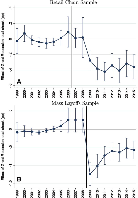
FIG.5.— Employment impacts in special samples. A, This graph replicates ﬁgure 4A in

the retail chain sample (all year-2006 nonheadquarters workers for identiﬁable retail chain

ﬁrms), with 2006 age-earnings-ﬁrm ﬁxed effects instead of 2006 age-earnings-industry ﬁxed

effects. The retail chain sample is reweighted to match the main sample as in DiNardo et al.

(1996), along 2007 CZ, gender, 5-year age bin, and 2006 earnings bins as deﬁned in ﬁgure 6.

Each fully interacted cell with overlap in both samples receives the same total weight in the

retail sample as in the main sample; the 0.02 percent of retail chain sample observations

with no overlap receive zero weight. Reweighting nearly halves the impact of ﬁrm ﬁxed ef-

fects (the difference between cols. 4 and 5 of table 4) and negligibly affects the ﬁnal point

estimate. B, This graph replicates ﬁgure 4A in the mass-layoffs sample (all workers who sep-

arated from a ﬁrm in a 2008 or 2009 mass layoff), also reweighted to match the main sam-

ple, as above, with a negligible effect on the ﬁnal point estimate. See the ﬁgure 4A legend

for speciﬁcation details.

This content downloaded from 136.152.029.121 on May 28, 2020 09:49:28 AM

All use subject to University of Chicago Press Terms and Conditions (http://www.journals.uchicago.edu/t-and-c).

TABLE 4

2015 Impacts of Great Recession (GR) Local Shocks, Retail Chain Sample: Outcome Relative to Pre-2007 Mean

N 5 865,954

A. Main Speciﬁcations: Employed in 2015 (pp)

(1) (2) (3) (4) (5) (6) (7) (8)

GR local shock 2.414 2.426 2.398 2.407 2.359 2.340 2.339

(.118) (.119) (.102) (.094) (.080) (.063) (.061)

Most severely shocked quintile 21.496

(.308)

Fourth shock quintile 21.416

(.298)

Third shock quintile 2.968

(.288)

Second shock quintile 2.366

(.298)

Age FEs X

Age-earnings FEs X

Age-earnings-industry FEs X

Age-earnings-ﬁrm FEs XXXX

Unemployment persistence in 2007 CZ X

Unemployment persistence in 2015 CZ X

.00 .00 .02 .03 .07 .15 .15 .15

Outcome mean 29.80 29.80 29.80 29.80 29.80 29.80 29.80 29.80

Absolute outcome mean 81.8 81.8 81.8 81.8 81.8 81.8 81.8 81.8

Standard deviation of GR local shocks 1.49 1.49 1.49 1.49 1.49 1.49 1.49 1.49

Interquartile range of GR local shocks 2.31 2.31 2.31 2.31 2.31 2.31 2.31 2.31

2536

This content downloaded from 136.152.029.121 on May 28, 2020 09:49:28 AM

All use subject to University of Chicago Press Terms and Conditions (http://www.journals.uchicago.edu/t-and-c).

B. Additional Outcomes and Controls

Cumulative Employment

2009–15 (pp)

(9)

Earnings

in 2015 ($)

(10)

Cumulative Earnings

2009–15 ($)

(11)

Employed in 2015 (pp)

(12) (13) (14)

GR local shock 22.504 2422 22,777 2.365 2.589 2.405

(.430) (134) (606) (.081) (.111) (.095)

Rust CZ  GR local shock .258 .069

(.144) (.115)

Other CZ  GR local shock .414

(.251)

Age-earnings-ﬁrm FEs X X X X X X

Manufacturing share X

.15 .21 .23 .15 .15 .15

Outcome mean 251.5 2,356 8,381 29.80 29.80 29.80

Absolute outcome mean 590.0 33,381 225,554 81.8 81.8 81.8

Standard deviation of GR local shocks 1.49 1.49 1.49 1.49 1.49 1.49

Interquartile range of GR local shocks 2.31 2.31 2.31 2.31 2.31 2.31

Note.—This table replicates table 2 in the retail chain sample. See the note to that table for details. “Firm” is an indicator for the individual’s 2006 ﬁrm (a

retail chain ﬁrm). The retail chain sample is reweighted to match the main sample, as described in the ﬁg. 5 legend.

2537

This content downloaded from 136.152.029.121 on May 28, 2020 09:49:28 AM

All use subject to University of Chicago Press Terms and Conditions (http://www.journals.uchicago.edu/t-and-c).

2015 point estimate from ﬁgure 5A. Relative to column 4’s estimate con-

trolling only for age-earnings-industry ﬁxed effects, one sees that the ﬁrm

ﬁxed effects attenuate the point estimate by 11.8 percent, or one-half of

one standard error.

If the paper’s main estimate of 20.393 is overstated

by 11.8 percent, then the true main-sample effect size would be 20.347.

The retail chain sample’s earnings effects are smaller than those in the

main sample, though 2015 mean earnings are also smaller in the retail

chain sample. Overall, results are similar across the main and retail chain

samples.

D. Extrapolation

I close the section with a simple extrapolation of the 2015 employment

impact of Great Recession local shocks to the 2015 employment impact

of the Great Recession aggregate shock. The exercise adopts the strong

“naive” assumption that the impact of the Great Recession aggregate

shock on national residents is identical to the impact of a proportionally

sized Great Recession local shock on initial local residents, as in similar

work (e.g., Charles, Hurst, and Notowidigdo 2015). I ﬁnd that simple ex-

trapolation suggests that the Great Recession caused 76 percent of the

postrecession age-adjusted decline in the working-age US employment

rate as measured in this paper (any annual employment of the birth co-

horts aged 30–49 in 2007).

The extrapolation estimate of 76 percent derives from three inputs.

First, the aggregate US unemployment rate increased by 4.63 percentage

points from 2007 to 2009. Second, table 2, column 4, reported that expo-

sure to a 1 percentage point higher local unemployment spike 2007–9 in-

duced a 0.393 percentage point decline in any 2015 employment. Based

on these two inputs, simple extrapolation suggests a 1.82 (4:63  0:393)

percentage point decline in the US working-age employment rate be-

cause of the Great Recession.

Third, the employment rate decline of these birth cohorts through

2015, 7.23 percentage points (table 2), was 2.40 percentage points larger

than the decline that would have been expected because of aging, based

on analogous earlier cohorts through years 2003–7. Speciﬁcally, recall

that 27:23 5 De

2015

, where De

; E½EMPLOYED

jcðiÞ ∈ C

 2 ð1=8Þo

t29

s5t216

E½EMPLOYED

jcðiÞ ∈ C

andthatC

isthesetofworking-agebirthcohorts

ft 2 58, … , t 2 39g. These cohorts would have experienced an employ-

ment rate decline due to aging even in the absence of the recession. I

quantify the aging effect by using employment rates of analogous earlier

working-age cohorts through years 2003–7asð1=5Þo

2007

t52003

De

524:83,

Introducing ﬁrm ﬁxed effects increased the effect magnitude in an earlier version’s

speciﬁcations.

2538 journal of political economy

This content downloaded from 136.152.029.121 on May 28, 2020 09:49:28 AM

All use subject to University of Chicago Press Terms and Conditions (http://www.journals.uchicago.edu/t-and-c).

based on the Current Population Survey’s Annual Social and Economic

Supplement (ASEC) in lieu of tax data availability before 1999. The age-

adjusted working-age employment rate decline was therefore 2.40 (7:232

4:83) percentage points. Hence, simple extrapolation suggests that the

GreatRecessioncaused76percent(1.82/2.40)oftheage-adjusteddecline.

It is important to note that the actual impact may be more or less than

76 percent. First, there is statistical and speciﬁcation uncertainty in the

2015 impact of Great Recession local shocks. Sections IV.A and IV.C de-

scribed scenarios in which one could believe that the true effect size was

closer to 0.3. When 0.300 is used instead of 0.393, the share explained by

the recession is 58 percent. Second, there is extrapolative uncertainty be-

cause of general equilibrium considerations (Nakamura and Steinsson

2014; Beraja et al. 2016). A shock to one local area can have a larger local

impact than a proportionately sized aggregate shock, for example, because

production can more easily shift across local areas than across countries.

Alternatively, the impact of an aggregate shock may exceed the impact of

a proportionately sized local shock on initial local residents, for exam-

ple, to the extent that initial local residents escaped or dampened local-

shock impacts by migrating to other local areas (Blanchard and Katz

1992) more than to other countries.

V. Impact Heterogeneity

This section analyzes impact heterogeneity across individuals. An active

literature in labor economics studies determinants of wage earnings in-

equality within (e.g., Card, Heining, and Kline 2013) and across (e.g.,

Autor, Katz, and Kearney 2008) worker types. The previous section found

that Great Recession local shocks caused 2015 wage earnings inequality

within worker types: initially similar workers experienced different 2015

employment and earnings outcomes after exposure to different Great Re-

cession local shocks. Figure 6 explores effects of Great Recession local

shocks on inequality across worker types.

Figure 6A displays employment impact heterogeneity. The ﬁgure’s ﬁrst

ﬁve rows plot point estimates and 95 percent conﬁdence intervals of the

2015 employment impact of Great Recession local shocks overall in the

main sample (reprinting the main estimate from table 2, col. 4) and in

each of four 2006 earnings bins, a common proxy for broad initial skill

level (e.g., Autor et al. 2014). I ﬁnd that low initial earners bore more of

the employment incidence of Great Recession local shocks, suggesting

Note that the age-adjusted decline of 2.40 percentage points is similar to the age-

adjusted declines in headline BLS point-in-time employment rates reported in the intro-

duction. To account for modest age distribution differences related to the baby boom,

cohorts underlying the computation of ð1=5Þo

2007

t52003

De

are reweighted to match the

working-age distribution for t 5 2015, as written in the appendix below.

employment hysteresis from the great recession 2539

This content downloaded from 136.152.029.121 on May 28, 2020 09:49:28 AM

All use subject to University of Chicago Press Terms and Conditions (http://www.journals.uchicago.edu/t-and-c).

FIG.6.— Impact heterogeneity. A, Coefﬁcients and 95 percent conﬁdence intervals (clus-

tering by 2007 state) of the impact of Great Recession local shocks on 2015 relative employ-

ment—overall and by subgroup. All estimates derive from the speciﬁcation underlying ﬁg-

ure 4A’s 2015 data point, corresponding here to the overall row. Subgroup estimates restrict

the sample to the speciﬁed subgroup deﬁned by 2006 earnings, 2003–6 labor force (LF) at-

tachment, 2007 age, gender, 2006 marital status, 2006 number of children, or 2006 mort-

gage holding. Non-1040-ﬁlers are classiﬁed here as single and childless. Subgroup migration

rates are superimposed on the right. Migration is deﬁned as one’s 2015 CZ being different

from one’s 2007 CZ. B, Replication of A for 2015 earnings, expressed in multiples of mean

annualearnings1999–2006:2015 earnings divided bymean annual 1999–2006 earnings. This

quantity is top-coded at the 99th percentile: individuals with zero 1999–2006 earnings are

assigned the top code if 2015 earnings were positive and assigned 0 otherwise. The overall es-

timate is 23.55 (standarderror: 0.94), implying that a 1 percentage point higher Great Reces-

sion local shock reduced the average individual’s 2015 earnings by 3.55 percent of her prere-

cession earnings.

This content downloaded from 136.152.029.121 on May 28, 2020 09:49:28 AM

All use subject to University of Chicago Press Terms and Conditions (http://www.journals.uchicago.edu/t-and-c).

that those shocks increased employment inequality across workers of dif-

ferent initial skill levels. Low initial earners (deﬁned as those who earned

less than $15,000 in 2006, approximately the 33rd percentile in this sam-

ple) experienced a worse than average impact, while high initial earners

(deﬁned as those who earned more than $45,000 in 2006, approximately

the 67th percentile) experienced a better-than-average impact. This cross-

area ﬁnding mirrors the earlier cross-time ﬁnding that aggregate em-

ployment declines since 2007 were concentrated among the least skilled

(Hoynes, Miller, and Schaller 2012; Charles et al. 2016). The subsequent

three rows suggest worse-than-average impacts among individuals with

less labor force attachment (Autor et al. 2014).

Figure 6B displays similar patterns for earnings. I analyze proportional

earnings changes in order to parallel earlier work on earnings inequality

studying earnings ratios, such as the ratio of the 90th and 50th percentiles

(Autor et al. 2008). Analogous to that of Autor et al. (2014), the outcome

in each regression is the ratio of 2015 earnings to mean annual pre-

2007 earnings with no local cost-of-living adjustments: EARNINGS

i2015

ð1=8Þo

2006

s51999

EARNINGS

The overall estimate indicates a large impact

of Great Recession local shocks on proportional earnings: a 1 percentage

point higher Great Recession local shock reduced the average individu-

al’s 2015 earnings by 3.55 percent of her prerecession earnings. The sub-

group analysis reveals relatively similar proportional earnings declines

across subgroups, except by initial earnings and labor force attachment

subgroups, where low initial earners and less-attached individuals experi-

enced larger declines. Hence, both employment and earnings analyses

suggest that Great Recession local shocks increased inequality across work-

ers of different initial skill levels.

The remaining rows of ﬁgure 6 display impact heterogeneity by gen-

der, 2007 age group, 2006 marital status, 2006 number of children, and

2006 mortgage holding status. I ﬁnd larger employment effects among

older individuals than among younger individuals—consistent with pre-

vious work suggesting that older workers are less resilient to labor market

shocks ( Jacobson et al. 1993).

Finally, one may expect that migration rate heterogeneity explains im-

pact heterogeneity, in light of the lesson from Blanchard and Katz (1992)

that population reallocation equilibrates US local labor markets. Figure 6

lists migration rates—deﬁned as the share of individuals with a 2015 CZ

different from their 2007 CZ—for each subgroup of individuals to the

right of the subgroup-speciﬁc impacts. There is no consistent correla-

tion between migration rates and estimated Great Recession local-shock

This quantity is very right skewed and therefore top coded at the 99th percentile. In-

dividuals with zero 1999–2006 earnings are assigned the top code if 2015 earnings were

positive and are assigned 0 otherwise.

employment hysteresis from the great recession 2541

This content downloaded from 136.152.029.121 on May 28, 2020 09:49:28 AM

All use subject to University of Chicago Press Terms and Conditions (http://www.journals.uchicago.edu/t-and-c).

impacts. For example, non–mortgage holders had an 18 percent migra-

tion rate, while mortgage holders had a 13 percent migration rate; yet,

if anything, non–mortgage holders appear to have experienced larger im-

pacts. The next section further explores adjustment via out-migration.

VI. Adjustment Margins

This paper’s rich administrative data allow me not only to estimate long-

term employment and earnings impacts but also to estimate year-by-year

adjustments across space and onto social-insurance programs. Table 5 an-

alyzes year-by-year adjustment margins. Each cell lists the coefﬁcient and

standard error on the Great Recession local-shock variable from a sepa-

rate regression in the main analysis sample with the main controls (2006

age-earnings-industry ﬁxed effects), varying only the outcome. Column 1

reproduces the 2007–15 employment estimates plotted in ﬁgure 4A. Col-

umn 2 analyzes migration, using a binary outcome equal to one if and only

if an individual’s residential CZ in the year was different from her 2007

CZ. The estimates indicate that individuals who experienced more severe

Great Recession local shocks were insigniﬁcantly (0.073 percentage points)

more likely to have moved after 2007 relative to the overall migration rate

of 16 percent, suggesting that out-migration was not a major adjustment

margin.

Columns 3 and 4 further support that conclusion by disaggregating the

annual employment results of column 1 into two types of annual employ-

ment: employment inside the individual’s 2007 CZ and employment out-

side the individual’s 2007 CZ, similar to Autor et al. (2014).

Unsurpris-

ingly, given the main effect of column 1, column 3 shows that individuals

subject to more severe Great Recession local shocks were signiﬁcantly less

likely to be employed in their 2007 CZs in 2015. But column 4 shows that

these individuals were insigniﬁcantly less likely to be employed outside

their 2007 CZs as well. Columns 5–7 show analogous results for earnings.

Column 7 shows a marginally signiﬁcant negative effect of Great Reces-

sion local shocks on out-of-2007-CZ earnings in 2015, implying no replace-

ment of lost 2015 within-initial-CZ earnings with earnings in other CZs at

the 95 percent conﬁdence upper bound.

The lack of an out-migration response may besurprising, giventhe ﬁnd-

ing of Section II that population fell relative to trend in severely shocked

states and by the same large magnitude predicted by Blanchard and Katz

(1992). However, population reallocation is consistent with substantially

That is, the col. 3 outcome for a year t equals ð1 2 MOVED

Þ EMPLOYED

ð1=8Þo

2006

s51999

EMPLOYED

,whereMOVED

(the col. 2 outcome) equals one if cðitÞ ≠ cði2007Þ

and zero otherwise. The col. 4 outcome for a year t equals MOVED



EMPLOYED

2 ð1=8Þo

2006

s51999

EMPLOYED

2542 journal of political economy

This content downloaded from 136.152.029.121 on May 28, 2020 09:49:28 AM

All use subject to University of Chicago Press Terms and Conditions (http://www.journals.uchicago.edu/t-and-c).

TABLE 5

Time Series of Adjustment Margins

Outcome (Relative or Absolute)

Employed

(pp)

(1)

Migrated outside

2007 CZ

(pp)

(2)

Employed

in 2007 CZ

(pp)

(3)

Employed outside

2007 CZ

(pp)

(4)

Earnings

($)

(5)

Earnings

in 2007 CZ

($)

(6)

Earnings outside

2007 CZ

($)

(7)

Income

($)

(8)

SSDI

Income

($)

(9)

Effect in 2007 .087 .000 .087 .000 2205 2205 0 14.3 23.8

(.106) (.106) (115) (115) (12.2) (8.9)

Effect in 2008 2.099 .036 2.098 2.001 2508 2480 228 36.3 23.4

(.079) (.119) (.077) (.006) (108) (108) (11) (15.6) (9.4)

Effect in 2009 2.349 .109 2.321 2.028 2750 2687 263 94.0 .5

(.080) (.208) (.077) (.012) (129) (127) (18) (32.1) (11.8)

Effect in 2010 2.403 .209 2.367 2.037 2807 2736 271 83.9 2.6

(.074) (.272) (.074) (.017) (131) (125) (30) (32.1) (13.0)

Effect in 2011 2.387 .248 2.339 2.048 2840 2745 2

94 43.1 7.5

(.072) (.296) (.071) (.022) (119) (105) (35) (24.3) (13.7)

Effect in 2012 2.373 .244 2.324 2.049 2890 2784 2106 19.9 9.8

(.075) (.334) (.076) (.026) (141) (117) (45) (20.1) (15.2)

Effect in 2013 2.434 .180 2.365 2.069 2960 2810 2149 7.7 13.0

(.089) (.382) (.091) (.032) (147) (108) (56) (16.3) (17.0)

Effect in 2014 2.360 .134 2.322 2.038 2968 2799 2169 23.0 15.7

(.100) (.422) (.101) (.031) (197) (135) (84) (9.9) (17.7)

Effect in 2015 2.393 .073 2.338 2.055 2997 2786 2211 25.9 19.6

(.097) (.456) (.100) (.042) (168) (108) (101) (8.9) (18.8)

Note.—This table expands on the speciﬁcations of table 2, cols. 4 and 9, whose results are reprinted here in the bottom rows of cols. 1 and 5, respec-

tively. Each cell reports the coefﬁcient on the Great Recession local-shock variable from a separate regression in which the outcome uses the postrecession

year indicated in the row, instead of exclusively using 2015, as in table 2. Every regression uses the same 1,357,974 observations underlying table 2. The

col. 1 outcome of relative employment is deﬁned in table 2, varying the postrecession year between 2007 and 2015. The col. 2 outcome is an indicator for

out-migration, equal to the individual’s year-f CZ being different from her 2007 CZ. Columns 3 and 4 separate the col. 1 outcome for year f into two

outcomes: employment in year f in the individual’s 2007 CZ and employment in year f outside the individual’s 2007 CZ, each minus mean 1999 –

2006 employment. The col. 5 outcome is deﬁned in table 2. Columns 7 and 8 separate the col. 5 outcome analogously to cols. 3–4. The col. 8 outcome

is the individual’s unemployment insurance beneﬁts in year f. The col. 9 outcome is the individual’s Social Security Disability Insurance beneﬁts in year f.

Standard errors (in parentheses) are clustered by 2007 state. See online appendix table 2 for pretrends.

This content downloaded from 136.152.029.121 on May 28, 2020 09:49:28 AM

All use subject to University of Chicago Press Terms and Conditions (http://www.journals.uchicago.edu/t-and-c).

reduced in-migration rather than substantially increased out-migration

(Monras 2015). Autor et al. (2014) similarly ﬁnd that out-migration was

not a major margin of adjustment to import competition. I leave to other

work why more individuals did not out-migrate or where they migrated

(Yagan 2014).

Columns 8 and 9 study adjustment via social-insurance transfer pay-

ments: UI beneﬁts and SSDI beneﬁts.

Unsurprisingly, individuals ex-

posed to larger Great Recession local shocks received signiﬁcantly higher

mean UI beneﬁts in 2008 –10 than those exposed to smaller local shocks.

However, Great Recession UI beneﬁts soon expired, and these individu-

als’ higher mean UI beneﬁts declined after 2010 to insigniﬁcantly lower

UI beneﬁts by 2015. Column 9 shows that individuals subject to Great Re-

cession local shocks accumulated rising, though insigniﬁcantly higher,

SSDI beneﬁts relative to those subject to smaller Great Recession local

shocks. Comparing the sum of the 2007–15 UI and SSDI income coefﬁ-

cients to the sum of the column 5 earnings coefﬁcients, one estimates that

elevated UI and SSDI transfer payments replaced 5.1 percent of lost earn-

ings: 4.2 percent from UI and 0.9 percent from SSDI. Focusing only on

2015 SSDI income, one estimates that it replaced 2.0 percent (19.6/997)

of lost 2015 earnings, rising to 5.6 percent at the 95 percent conﬁdence

upper bound.

Thus, observed transfer payments far from fully compen-

sated for the negative earnings effects.

SSDI has been found to be an important margin of adjustment to labor

market shocks (Autor and Duggan 2003; Autor et al. 2013, 2014). Expand-

ing on table 5’s null SSDI results, table 6, column 1, replicates the paper’s

main speciﬁcation for the binary outcome of SSDI receipt in 2015. I ﬁnd

a moderate and insigniﬁcant estimated impact, though with substantial

uncertainty: a point estimate of 0.071 percentage points and a standard

error of 0.145 percentage points, relative to the employment impact of

20.393 percentage points.

More thoroughly, one can estimate the share of the incrementally non-

employed in severely shocked areas who were on SSDI in 2015. Table 6,

UI provides temporary cash beneﬁts to laid-off workers who had earned above a min-

imum threshold in the quarters preceding layoff. SSDI provides typically permanent (until

retirement age) cash and medical beneﬁts to individuals with at least 5 years of work history

in the 10 years before the individual developed a long-lasting medical condition deemed to

prevent substantial employment.

To estimate the upper bound, I regress 2015 SSDI on 2015 relative earnings instru-

mented with Great Recession local shocks, controlling for 2006 age-earnings-industry ﬁxed

effects and clustering on 2007 state. The coefﬁcient on 2015 relative earnings is 20.020,

with a standard error of 0.018.

Spousal labor supply was likely also a ver y incomplete adjustment margin: the shocks

studied here are measured as CZ-wide shocks, both genders and marital statuses suffered

large impacts (ﬁg. 6), and earlier work in similar data showed that wives replaced only

5.6 percent of males’ lost income after layoff (Hilger 2016).

2544 journal of political economy

This content downloaded from 136.152.029.121 on May 28, 2020 09:49:28 AM

All use subject to University of Chicago Press Terms and Conditions (http://www.journals.uchicago.edu/t-and-c).

column 2, estimates the effect of Great Recession local shocks on a new

outcome similar to that of Lee (2009): an indicator for whether the worker

was employed in 2015 or received SSDI in 2015, m inus mea n employ -

ment 1999–2006.

Table 6, column 2, reports that Great Recession lo-

cal shocks had a signiﬁcant negative effect, 20.265 percentage points,

on the employed-or-SSDI outcome, suggesting that 32.6 percent (12

ð20:265=20:393Þ) of the incrementally nonemployed received SSDI in

2015. However, the standard errors are substantial.

The potentially modest role of SSDI in absorbing individuals after

Great Recession local shocks is consistent with aggregate patterns. The

share of age-16–65 Americans on SSDI rose for three decades before de-

celerating after 2010 and declining absolutely in both 2014 and 2015. Ag-

gregate SSDI applications spiked after the Great Recession, as they have

after previous recessions, but Maestas, Mullen, and Strand (2015) use data

through 2012 to estimate that virtually all of the Great Recession–induced

applications were initially declined. SSDI application is not observed in

this paper’s data.

VII. Layoffs and Nonemployment Trajectories

Table 5 showed that statistically signiﬁcant nonemployment effects be-

gan in 2009 and that there were statistically signiﬁcant effects on UI ben-

eﬁts 2008–10. A large literature connects layoffs and long-term earnings

losses (Topel 1990; Ruhm 1991; Jacobson et al. 1993; Neal 1995; Kahn

2010; Davis and von Wachter 2011). I therefore provide additional evi-

dence on layoffs and long-term employment losses.

Table 6, column 6, replicates the main speciﬁcation for the binary out-

come of ever having received UI in 2007–14—a good proxy for everhaving

been laid off in 2007–14.

The column indicates that a 1 percentage point

higher Great Recession local shock induced individuals to be 1.43 per-

centage points more likely to receive UI in 2007–14, with a t-statistic over

3 and relative to the sample mean of 25.6 percent.

The substantial 2007–14 layoff effect relative to the 2015 employment

effect suggests that most of the incrementally nonemployed from severely

shocked areas may have been laid off. Column 7 conﬁrms that suggestion.

Analogous to column 2’s employed-or-on-SSDI analysis, column 7 repli-

cates the main speciﬁcation on a new outcome: an indicator for whether

That is, the outcome equals maxfEMPLOYED

i2015

, SSDI

i2015

g 2 ð1=8Þo

2006

s51999

EMPLOYED

, where SSDI

i2015

equals one if i received SSDI in 2015 and zero otherwise.

Kawano and LaLumia (2017) show that UI-tax-data-based unemployment rates are

close in both level and trend to ofﬁcial BLS unemployment rates for 1999–2011 (correla-

tion: 0.94). Earlier papers typically proxy for layoff by using ﬁrm separation during a ﬁrm’s

large downsizing; my measure here is not limited to large downsizings.

employment hysteresis from the great recession 2545

This content downloaded from 136.152.029.121 on May 28, 2020 09:49:28 AM

All use subject to University of Chicago Press Terms and Conditions (http://www.journals.uchicago.edu/t-and-c).

TABLE 6

Additional Outcomes

A. Disability Insurance Receipt in Main Sample (pp) B. Employment Impacts in Mass Layoffs Sample (pp)

SSDI Receipt

in 2015

(1)

2015 Relative Employment

or SSDI Receipt

(2)

2015 Relative

Employment

(3)

2015 Relative

Employment

(4)

2015 Relative

Employment

(5)

Great Recession local

shock .071 2.265 2.577 2.628 2.605

(.145) (.099) (.126) (.118) (.125)

Main controls X X X X X

Exclude if invalid

industry code XX

Exclude if construction/

manufacturing X

Observations 1,357,974 1,357,974 1,001,543 573,493 396,377

.12 .09 .11 .17 .15

Outcome mean 6.22 22.28 210.12 210.45 29.85

Absolute outcome mean 6.22 84.06 84.12 83.11 83.20

2546

This content downloaded from 136.152.029.121 on May 28, 2020 09:49:28 AM

All use subject to University of Chicago Press Terms and Conditions (http://www.journals.uchicago.edu/t-and-c).

C. Layoffs and Nonemployment in Main Sample

UI Receipt Some-

time 2007–14

(6)

2015 Relative Employment or

UI Receipt Sometime 2007–14

(7)

2015 Relative

Employment

(8)

Relative Nonemployment

2007–14

(9)

2015 Relative

Employment

(10)

2013–15Relative

Employment

(11)

Great Recession local

shock 1.431 2.019 2.354 .487 2.057 2.285

(.418) (.121) (.099) (.122) (.111) (.101)

UI receipt sometime

2007–14 22.734

(.142)

Main controls X X X X X X

Employment 2007–12 X

Observations 1,357,974 1,357,974 1,357,974 1,357,974 1,357,974 1,357,974

.16 .06 .08 .08 .26 .07

Outcome mean 25.6 22.8 27.2 3.0 27.2 21.2

Absolute outcome mean 25.6 83.6 79.1 3.0 79.1 85.2

Note.—The table reports estimates of the speciﬁcation in table 2, col. 4, with alternative outcomes, samples, and/or controls. Column 1 replicates the main

speciﬁcation, using the outcome of an indicator for 2015 receipt of Social Security Disability Insurance. Column 2 replicates the main speciﬁcation, using the

outcome of an indicator for 2015 employment or 2015 SSDI receipt, minus the individual’s mean employment 1999–2006. Column 3 replicates the main spec-

iﬁcation, and cols. 4 –5 replicate table 3, cols. 11–12, in the mass-layoffs sample. Column 6 replicates the main speciﬁcation, using the outcome of an indicator

for unemployment insurance beneﬁt receipt at some point 2007–14. Column 7 replicates col. 2 but uses UI receipt in 2007–14 in place of 2015 SSDI receipt.

Column 8 replicates the main speciﬁcation, controlling for UI receipt sometime in 2007–14. Column 9 replicates the main speciﬁcation, using the outcome of

an indicator for having any year of nonemployment during 2007–14, minus an indicator for having any year of nonemployment 1999–2006. Column 10 rep-

licates the main speciﬁcation while controlling for indicators of employment in each year 2007–12. Column 11 replicates the main speciﬁcation, using the

outcome of an indicator for employment in any year 2013–15, minus the individual’s mean employment 1999–2006. Standard errors (in parentheses) are clus-

tered by 2007 state.

2547

This content downloaded from 136.152.029.121 on May 28, 2020 09:49:28 AM

All use subject to University of Chicago Press Terms and Conditions (http://www.journals.uchicago.edu/t-and-c).

the individual was employed in 2015 or received UI at some point in 2007–

14, minus the individual’s mean employment status in 1999–2006. The

column 7 estimate is nearly zero and indicates that Great Recession local

shocks had no statistically signiﬁcant impact on the employed-or-UI out-

come. Hence, most of the incrementally nonemployed from severely

shocked areas had been laid off.

The preceding ﬁndings may suggest that the initial residents of severely

shocked areas suffered higher rates of 2015 nonemployment purely be-

cause those residents were laid off from their initial jobs at higher rates.

Two pieces of evidence suggest that that is not the case. First, column 8

replicates the main speciﬁcation while controlling for the indicator of

ever receiving UI 2007–14. The Great Recession local-shock coefﬁcient

is barely attenuated, indicating that effects hold within layoff status. It

is easy to see why quantitatively: multiplying the coefﬁcient on UI receipt

(22.73) by the higher rate of UI receipt (1.43) yields the 0.04 percentage

point attenuation in the main estimate. Layoff status is endogenous, but

with homogeneous layoff effects and under the mild monotonicity con-

dition that the marginally laid off in severely shocked areas had weakly

better unobservables (Gibbons and Katz 1991), this result suggests that

layoff effects are not nearly large enough for a 1.43 percentage point higher

layoff rate to explain the 2015 employment effect.

More simply, ﬁgure 5B replicates ﬁgure 4A in the mass-layoffs sample—

thereby comparing the employment rates of workers who were displaced

in 2008–9 mass-layoff events at the same age, in the same initial earnings

bin, and in the same initial industry but in different local areas. If layoff ef-

fects were homogenous across space and severely shocked areas simply ex-

perienced more layoffs—and if the incrementally displaced in severely

shocked areas were no worse on unobservables (Gibbons and Katz)—then

one would not ﬁnd a negative 2015 employment effect in the mass-layoffs

sample. Yet ﬁgure 5B shows that individuals in the mass-layoffs sample

were 0.577 percentage points less likely to be employed in 2015 for every

1 percentage point higher Great Recession local shock. This result (also

reported in table 6, col. 3) is robust to restricting the sample to mass-layoff

ﬁrmswithvalidindustry codes,includingthoseoutsidemanufacturingand

construction (cols. 4–5). This evidence suggests that this paper’s 2015

nonemployment effects are not explained purely by higher layoff rates

and parallels work on larger earnings impacts in weak local ( Jacobson

et al. 1993) and aggregate (Davis and von Wachter 2011) labor markets.

Under homogenous layoff effects and the monotonicity condition, the UI receipt co-

efﬁcient weakly overstates the layoff effect for workers from severely shocked areas, suggest-

ing that the magnitude of the shock coefﬁcient is a lower bound on the true effect net of

the layoff effect.

2548 journal of political economy

This content downloaded from 136.152.029.121 on May 28, 2020 09:49:28 AM

All use subject to University of Chicago Press Terms and Conditions (http://www.journals.uchicago.edu/t-and-c).

Columns 9–11 of table 6 return to the main sample to document con-

tinuous nonemployment trajectories. Column 9 replicates the main spec-

iﬁcation for the outcome of an indicator for whether the individual was

nonemployed for any year 2007–14, minus an indicator for whether the

individual was nonemployed for any year 1999–2006. The estimated co-

efﬁcient implies that Great Recession local shocks resulted in the average

working-age American being 0.487 percentage points more likely to ex-

perience a full year of nonemployment in 2007–14. Column 10 shows

thatpre-2015 nonemploymentstatisticallyexplains2015nonemployment:

there is no statistically signiﬁcant correlation between Great Recession lo-

cal shocks and 2015 relative employment once one controls additively for

indicators of employment in each year 2007–12. Column 11 replicates the

main speciﬁcation for the outcome of an indicator for whether the indi-

vidual was employed in any year 2013–15, minus the individual’s mean

employment in 1999–2006. The estimate is 20.285, with a t-statistic of 2.8.

Thus, the point estimates in columns 9–11 suggest that 2015 employment

impacts typically followed an annual nonemployment impact in 2007–12

and constituted a third consecutive year of nonemployment impacts.

VIII. Discussion of Mechanisms

The previous section found that one candidate channel—higher layoff

rates with homogenous layoff effects—likely does not explain the paper’s

results. I close with brief further discussion of six candidate mechanisms:

reduced migration, higher reservation wages on SSDI, lost job-speciﬁc

rents, lost ﬁrm-speciﬁc human capital, general human capital decay, and

persistently low labor demand. Higher reservation wages on SSDI could

explain a sizable portion of the impact. General human capital decay and

persistently low labor demand could explain the full impact.

Reduced migration could in principle explain long-term impacts of

Great Recession local shocks, relative to other local shocks, but does not

appear to do so. First, and despite the possibility of negative-equity mort-

gages impeding homeowner out-migration (Ferreira, Gyourko, and Tracy

2010, 2011), several papers have argued that the Great Recession did not

impede migration (Farber 2012; Schulhofer-Wohl 2012; Valletta 2013;

Şahin et al. 2014). Second, Section II found that 2007–15 population real-

location was in line with historical responses. Third, ﬁgure 6 found that

impact heterogeneity across demographic groups was not systematically

correlated with group migration rates—consistent with, though not dis-

positive of, a hypothetically higher out-migration rate attenuating little

incidence.

The Great Recession could have induced individuals to supplement their

income with SSDI—a costly-to-obtain but typically permanent location-

independent income stream—thereby raising their reservation wages and

employment hysteresis from the great recession 2549

This content downloaded from 136.152.029.121 on May 28, 2020 09:49:28 AM

All use subject to University of Chicago Press Terms and Conditions (http://www.journals.uchicago.edu/t-and-c).

potentially reducing their employment (Autor and Duggan2003; Maestas,

Mullen, and Strand 2013).

Reservation wages are not observed, but the

SSDI channel appears to explain a minority of the results. Column 1 of

table 6 estimated that Great Recession local shocks caused insigniﬁcantly

higher 2015 SSDI enrollment, with a point estimate equal to one-ﬁfth of

the main employment effect, while column 2 estimated that one-third of

the incrementally nonemployed were on SSDI in 2015, though with sub-

stantial standard errors. An important caveat is that applying for SSDI

effectively requires nonemployment, so the data are consistent with stra-

tegic labor force exit in order to apply for beneﬁts, even if strategic appli-

cation was unsuccessful through 2015.

Laid-off workers will choose to remain nonemployed after losing a high-

paying rent-sharing job if subsequent wage offers lie below the worker’s

reservation wage.

Lost job-speciﬁc rents do not appear to explain the re-

sults. First, the 2015 impact of Great Recession local shocks is large not

only in the main sample but also in the retail chain sample—even though

retail is a canonical low-rent industry (Krueger and Summers 1988; Katz

and Summers 1989; Murphy and Topel 1990; Gibbons and Katz 1991).

Second, ﬁgure 6 showed that the largest impacts were suffered by those with

the lowest initial earnings, where the scope for rents was likely low. Third

and most simply, the same ﬁgure shows that the estimated 2015 nonem-

ployment impact appears large for those who had no earnings at all in

2006 and thus certainly had been earning no rents.

A worker losing a job for which she had ﬁrm-speciﬁc human capital

will choose to remain nonemployed if the worker’s marginal product—

and thus wage at the next-best ﬁrm —lies below her reservation wage

(Topel 1990; Jacobson et al. 1993). Lost ﬁrm-speciﬁc human capital at lay-

off does not appear to explain the results, as the quantitative results re-

main essentially intact within displaced individuals (table 6, cols. 5–8;

ﬁg. 5B). The incrementally laid off in severely shocked areas seem likely

to have had weakly better unobservables, as employers may lay off the un-

observably worst workers ﬁrst (Gibbons and Katz 1991). Hence, heteroge-

neous layoff effects—with the incrementally laid off being less resilient to

their loss of ﬁrm-speciﬁc human capital—appear necessary for the ﬁrm-

speciﬁc human capital channel to explain the results.

The results appear consistent with general human capital decay and

persistently low labor demand. Severe recessions generate relatively long

Recipients forfeit their income streams if they return to substantial work.

Motivated by the union wage premium (e.g., Lewis 1963; Farber 1986), some empir-

ical commentary has interpreted postlayoff earnings losses as reﬂecting workers’ loss of

rents in an initial job that paid above the worker’s marginal product (e.g., Hall 2011). Pre-

existing contrary evidence includes that postlayoff earnings losses are large and signiﬁcant

across both high-apparent-rent and low-apparent-rent industries ( Jacobson et al. 1993).

2550 journal of political economy

This content downloaded from 136.152.029.121 on May 28, 2020 09:49:28 AM

All use subject to University of Chicago Press Terms and Conditions (http://www.journals.uchicago.edu/t-and-c).

nonemployment spells, and general human capital can decay during such

spells (Phelps 1972), leading to persistent nonemployment (Pissarides

1992), such as via job ladders with serially correlated unemployment spells

( Jarosch 2015). For example, workers may fail to keep up with new tech-

nologies or preserve good habits such as punctuality and then may choose

nonparticipation over lower-wage employment ( Juhn, Murphy, and Topel

1991, 2002). Consistent with general human capital decay, columns 1 and

9–11 of table 6 found that incremental 2015 nonemployment typically

followed a layoff and multiple years of nonemployment in 2007–14. Gen-

eral human capital decay after a prolonged nonemployment spell is also

consistent with earlier ﬁndings of reduced long-term earnings after mass

layoffs in weak local ( Jacobson et al. 1993) and aggregate (Davis and von

Wachter 2011) labor markets.

Alternatively, severely shocked areas may have experienced persistently

low labor demand, and mobility frictions may have resulted in initial resi-

dents bearing the incidence (Kline 2010; Moretti 2011).

First, local Great

Recession–driving processes (e.g., spending contractions or productivity

shocks) could have been persistent, causing wages to fall below reserva-

tion wages (Hall 1992; Kline and Moretti 2014).

Second, transitory Great

Recession local shocks may have reduced the opportunity costs for agents

to respond to exogenous nationwide skill-biased or routine-biased techni-

calprogress( JaimovichandSiu[2012],withrecentempiricalsupportfrom

Hershbein and Kahn [2016])—accelerating wage declines below reser-

vationwages. Third,transitoryGreat Recession localshocksmayhavemoved

local areas to low-employment equilibria (Diamond 1982; Blanchard and

Summers 1986; Benhabib and Farmer 1994; Christiano and Harrison 1999;

Eggertsson and Krugman 2012; Kaplan and Menzio 2014), where neither

workers norﬁrms search forjob matcheseventhough both would gain from

trade at the prevailing wage. To the extent that the ﬁrst and last cases are

reversible, they are consistent with “hidden slack” among labor force non-

participants. All three cases are consistent with the results, including the

result that most of the incrementally nonemployed had been laid off.

Laid-off workers may be exactly those individuals whose wages fell below

reservation wages, or layoffs may have determined which speciﬁc workers

lost out in the new equilibrium without determining how many did.

Every decennial census shows that over two-thirds of adults live in their birth state

(Molloy et al. 2011). The Health and Retirement Study shows that half of adults live within

18 miles of their mot hers ( http://www.nytimes.co m/interactive/2 015/12/24 /upshot

/24up-family.html).

For example, with only nontradable production, net worth contractions (Mian and

Suﬁ 2014) could have permanently caused residents to shift to home production (Ben-

habib, Rogerson, and Wright 1991; Aguiar and Hurst 2005), reducing per capita local labor

demand and equilibrium wages below reservation wages.

employment hysteresis from the great recession 2551

This content downloaded from 136.152.029.121 on May 28, 2020 09:49:28 AM

All use subject to University of Chicago Press Terms and Conditions (http://www.journals.uchicago.edu/t-and-c).

General human capital decay leaves individuals changed (“scarred”),

while persistently low labor demand leaves local areas changed. Thus,

unique to the persistently-low-labor-demand mechanism, exogenously

moving individuals in 2015 from severely shocked to mildly shocked areas

may increase their employment rate. Future work could therefore distin-

guish between these mechanisms, with strong migration instruments that

generate quasi-experimental variation in individuals’ 2015 local areas.

IX. Conclusion

This paper used local labor markets as a laboratory to test for long-term

employment impacts of the Great Recession. The central ﬁnding is that

exposure to a severe local Great Recession caused working-age Americans

to be substantially less likely to be employed at all in 2015, despite recovery

in the local unemployment rate. This ﬁnding contrasts with the conven-

tional view that a business cycle’s employment impacts cease once unem-

ployment recovers. Instead, the Great Recession altered unemployment-

constant employment.

The paper highlights ﬁve areas for future work. First, the results sug-

gest the importance of allowing for labor force exit in models of macro-

economic ﬂuctuations (Mortensen and Pissarides 1999).

Such models

have the potential to show countercyclical policies to be relatively ﬁscally

inexpensive or even self-ﬁnancing, to the extent that they persistently in-

crease employment and earnings and thereby tax revenue (DeLong and

Summers 2012). Second, higher layoff rates do not appear to explain the

results, as the impacts hold within a sample of laid-off individuals, point-

ing instead to interactions with area-level economic conditions. Future

analysescouldfurthertestamongmechanisms.Third,newworkcouldinves-

tigate whether previous recessions also depressed long-term employment.

Fourth, naive extrapolation of the paper’s local-shock-based estimate

to the aggregate would suggest that the Great Recession caused over half

In addition, there are other potential mechanisms. For example, workers may have

made costly investments, such as moving in with one’s parents (Kaplan 2012) or honing

leisure skills (Aguiar et al. 2017), during nonemployment spells that then induced labor

supply contraction. However, nominal and real hourly wages declined rather than rose

in severely shocked areas (Beraja et al. 2016). Employers may have inferred low unobserved

productivity from long nonemployment spells, though such inference was smallest in se-

verely shocked areas (Kroft, Lange, and Notowidigdo 2013).

This conclusion includes the possibility that the recession ended a period of unsus-

tainable unemployment-constant employment, returning the economy to its pre-2000s

trend (Charles et al. 2016).

From Mortensen and Pissarides (1999, 1173): “Despite a ﬂurry of activity [in search

and matching theory] since [the early 1980s], there are still many important questions that

are unexplored. One such question is the dynamics of worker movement in and out of the

labor force. ...Virtually all search equilibrium models assume an exogenous labor force.”

Pissarides (1992) models search intensity that declines with unemployment duration.

2552 journal of political economy

This content downloaded from 136.152.029.121 on May 28, 2020 09:49:28 AM

All use subject to University of Chicago Press Terms and Conditions (http://www.journals.uchicago.edu/t-and-c).

of the 2007–15 age-adjusted decline in US working-age employment. Sub-

sequent analysis could determine whether the true aggregate impact was

less or more. Finally, employment impacts through 2015 do not imply

employment impacts forever, and it will be valuable to estimate and ex-

plain subsequent dynamics. For example, the age-25–54 US headline em-

ployment rate rose 1.6 percentage points from the beginning of 2016 to

the end of 2017, primarily via labor force entry. This upward 2016–17 em-

ployment trend could reﬂect continued cyclical recovery, with there hav-

ing been “hidden slack” among labor force nonparticipants who subse-

quently reentered the labor force in 2016–17 (Bell and Blanchﬂower,

forthcoming). The hidden-slack explanation is consistent with low wage

growth in 2016–17 and would indicate that the Great Recession’srecovery

extended anomalously long relative to previous cycles (cf. Fernald et al.

2017). Alternatively, it is possible that the recent upward employment trend

reﬂects up-skilling, a new positive aggregate shock, or another force.

Appendix

The working-age population (ages 30– 49 in any given year) has grown older over

time because of the baby boom. To account for this age distribution change, the

extrapolation exercise of Section IV.D uses the following formula to compute

each element in the summation ð1=5Þo

2007

t52003

De

c∈C

E EMPLOYED

jciðÞ5 c½2

t29

s5t216

E EMPLOYED

jciðÞ5 c½



where C

is the set of birth cohorts ft 2 58, … , t 2 39g and the cohort-reweighting

term l

is the population share of cohort c 1 2015 2 t in C

2015

in the March 2016

ASEC. When computing De

without cohort reweighting and thus simply

as E½EMPLOYED

jcðiÞ ∈ C

 2 ð1=8Þo

t29

s5t216

E½EMPLOYED

jcðiÞ ∈ C

, one obtains

ð1=5Þo

2007

t52003

De

524:22 instead of the 24.83 percentage points reported in the

text—which would reduce the exercise’s ﬁnal estimate from 76 percent to 61 per-

cent. ASEC data are limited to the civilian noninstitutional population. The vari-

able EMPLOYED

in ASEC is deﬁned as an afﬁrmative answer to either of two

questions asked of respondents in March of t 1 1: “Did [person] work at a job

or business at any time during [t]?” and “Did [person] do any temporary, part-

time, or seasonal work even for a few days during [t]?”

References

Aguiar, Mark, Mark Bils, Kerwin Charles, and Erik Hurst. 2017. “Leisure Luxuries

and the Labor Supply of Young Men.” Working Paper no. 23552 ( June), NBER,

Cambridge, MA.

Aguiar, Mark, and Erik Hurst. 2005. “Consumption versus Expenditure.” J.P.E.

113 (5): 919–48.

Autor, David H., David Dorn, and Gordon H. Hanson. 2013. “The China Syn-

drome: Local Labor Market Effects of Import Competition in the United

States.” A.E.R. 103 (6): 2121–68.

employment hysteresis from the great recession 2553

This content downloaded from 136.152.029.121 on May 28, 2020 09:49:28 AM

All use subject to University of Chicago Press Terms and Conditions (http://www.journals.uchicago.edu/t-and-c).

Autor, David H., David Dorn, Gordon H. Hanson, and Jae Song. 2014. “Trade

Adjustment: Worker-Level Evidence.” Q.J.E. 129 (4): 1799–1860.

Autor, David H., and Mark G. Duggan. 2003. “The Rise in the Disability Rolls and

the Decline in Unemployment.” Q.J.E. 118 (1): 157–205.

Autor, David H., Lawrence F. Katz, and Melissa S. Kearney. 2008. “Trends in US

Wage Inequality: Revising the Revisionists.” Rev. Econ. and Statis. 90 (2): 300–

23.

Bell, David, and David Blanchﬂower. Forthcoming. “Underemployment in Eu-

rope and the United States.” Indus. and Labor Relations Rev. https://www

.dartmouth.edu/~blnchﬂr/Projects.html.

Benhabib, Jess, and Roger E. A. Farmer. 1994. “Indeterminacy and Increasing

Returns.” J. Econ. Theory 63 (1): 19–41.

Benhabib, Jess, Richard Rogerson, and Randall Wright. 1991. “Homework in

Macroeconomics: Household Production and Aggregate Fluctuations.” J.P.E.

99 (6): 1166–87.

Beraja, Martin, Erik Hurst, and Juan Ospina. 2016. “The Aggregate Implications

of Regional Business Cycles.” Working Paper no. 21956 (February), NBER,

Cambridge, MA.

Black, Dan, Kermit Daniel, and Seth Sanders. 2002. “The Impact of Economic

Conditions on Participation in Disability Programs: Evidence from the Coal

Boom and Bust.” A.E.R. 92 (1): 27–50.

Blanchard, Olivier J., and Lawrence F. Katz. 1992. “Regional Evolutions.” Brook-

ings Papers Econ. Activity 1992 (1): 1–61.

Blanchard, Olivier J., and Lawrence H. Summers. 1986. “Hysteresis and the Eu-

ropean Unemployment Problem.” In NBER Macroeconomics Annual 1986,edited

by Stanley Fischer, 15–90. Cambridge, MA: MIT Press (for NBER).

Bowen, William G., and Aldrich T. Finegan. 1969. “Unemployment and Labor

Force Participation: Time-Series Relations.” In The Economics of Labor Force Par-

ticipation, chap. 16. Princeton, NJ: Princeton Univ. Press.

Card, David, Jörg Heining, and Patrick Kline. 2013.

“Workplace Heterogeneity

and the Rise of West German Wage Inequality.” Q.J.E. 128 (3): 967– 1015.

Charles, Kerwin Koﬁ, Erik Hurst, and Matthew J. Notowidigdo. 2015. “Housing

Booms and Busts, Labor Market Opportunities, and College Attendance.”

Working Paper no. 21587 (September), NBER, Cambridge, MA.

———. 2016. “The Masking of the Decline in Manufacturing Employment by

the Housing Bubble.” J. Econ. Perspectives 30 (2): 179–200.

Charles, Kerwin Koﬁ, Erik Hurst, and Mariel Schwartz. 2018. “The Transforma-

tion of Manufacturing and the Decline in U.S. Employment.” Working Paper

no. 24468 (March), NBER, Cambridge, MA.

Chetty, Raj, Nathaniel Hendren, Patrick Kline, and Emmanuel Saez. 2014.

“Where Is the Land of Opportunity? The Geography of Intergenerational

Mobility in the United States.” Q.J.E. 129 (4): 1553– 1623.

Christiano, Lawrence J., and Sharon G. Harrison. 1999. “Chaos, Sunspots and

Automatic Stabilizers.” J. Monetary Econ. 44 (1): 3–31.

Clemens, Jeffrey , and Michael Wither. 2014. “The Minimum W age and the Great Re-

cession: Evidence of Effects on the Employment and Income Trajectories of Low-

Skilled Workers.” Wo rking Paper no. 20724 (December), NBER, Cambridge, MA.

Dao, Mai, Davide Furceri, and Prakash Loungani. 2017. “Regional Labor Market

Adjustment in the United States: Trend and Cycle.” Rev. Econ. and Statis. 99 (2):

243–57.

Davis, Steven J., and Till von Wachter. 2011. “Recessions and the Costs of Job

Loss.” Brookings Papers Econ. Activity 2011 (2): 1–55.

2554 journal of political economy

This content downloaded from 136.152.029.121 on May 28, 2020 09:49:28 AM

All use subject to University of Chicago Press Terms and Conditions (http://www.journals.uchicago.edu/t-and-c).

Decressin, Jörg, and Antonio Fatas. 1995. “Regional Labor Market Dynamics in

Europe.” European Econ. Rev. 39 (9): 1627–55.

DeLong, J. Bradford, and Lawrence H. Summers. 2012. “Fiscal Policy in a De-

pressed Economy.” Brookings Papers Econ. Activity 2012 (Spring): 233–97.

Diamond, Peter A. 1982. “Aggregate Demand Management in Search Equilib-

rium.” J.P.E. 90 (5): 881–94.

DiNardo, John, Nicole M. Fortin, and Thomas Lemieux. 1996. “Labor Market In-

stitutions and the Distribution of Wages, 1973–1992: A Semiparametric Ap-

proach.” Econometrica 64 (5): 1001– 44.

Dorn, David. 2009. “Essays on Inequality, Spatial Interaction, and the Demand

for Skills.” PhD thesis, Univ. St. Gallen.

Eggertsson, Gauti B., and Paul Krugman. 2012. “Debt, Deleveraging, and the Li-

quidity Trap: A Fisher-Minsky-Koo Approach.” Q. J.E. 127 (3): 1469–1513.

Farber, Henry S. 1986. “The Analysis of Union Behavior.” In Handbook of Labor

Economics, vol. 2, edited by Orley C. Ashenfelter and Richard Layard, 1039–

89. Amsterdam: North-Holland.

———. 2012. “Unemployment in the Great Recession: Did the Housing Market

Crisis Prevent the Unemployed from Moving to Take Jobs?” A.E.R. 102 (3):

520–25.

Fernald, John G., Robert E. Hall, James H. Stock, and Mark W. Watson. 2017.

“The Disappointing Recovery of Output after 2009.” Brookings Papers Econ. Ac-

tivity 2017 (Spring): 1–58.

Ferreira, Fernando, Joseph Gyourko, and Joseph Tracy. 2010. “Housing Busts

and Household Mobility.” J. Urban Econ. 68 (1): 34–45.

———. 2011. “Housing Busts and Household Mobility: An Update.” Working Pa-

per no. 17405 (September), NBER, Cambridge, MA.

Gibbons, Robert, and Lawrence F. Katz. 1991. “Layoffs and Lemons.” J. Labor

Econ. 9 (4): 351–80.

Hall, Robert. 1992. “Comment on ‘Regional Evolutions’ by Blanchard and Katz.”

Brookings Papers Econ. Activity 1992 (1): 62–65.

———. 2011. “Comment on ‘Recessions and the Costs of Job Loss’ by Davis and

Von Wachter.” Brookings Papers Econ. Activity 2011 (2): 56–61.

Hershbein, Brad, and Lisa B. Kahn. 2016. “Do Recessions Accelerate Routine-

Biased Technological Change?” Working Paper no. 22762 (October), NBER,

Cambridge, MA.

Hilger, Nathaniel G. 2016. “ Parental Job Loss and Children’s Long-Term Out-

comes: Evidence from 7 Million Fathers’ Layoffs.” American Econ. J.: Appl. Econ.

8 (3): 247–83.

Hoynes, Hilary, Douglas L. Miller, and Jessamyn Schaller. 2012. “Who Suffers

During Recessions?” J. Econ. Perspectives 26 (3): 27–47.

Jacobson, Louis S., Robert J. LaLonde, and Daniel G. Sullivan. 1993. “Earnings

Losses of Displaced Workers.” A.E.R. 83 (4): 685–709.

Jaimovich, Nir, and Henry E. Siu. 2012. “The Trend Is the Cycle: Job Polarization

and Jobless Recoveries.” Working Paper no. 18334 (August), NBER, Cam-

bridge, MA.

Jarosch, Gregor. 2015. “Searching for Job Security and the Consequences of Job

Loss.” Manuscript, Univ. Chicago.

Juhn, Chinhui, Kevin M. Murphy, and Robert H. Topel. 1991. “Why Has the Nat-

ural Rate of Unemployment Increased over Time?” Brookings Papers Econ. Activ-

ity 1991 (2): 75–142.

———. 2002. “Current Unemployment, Historically Contemplated.

” Brookings

Papers Econ. Activity 2002 (1): 79–116.

employment hysteresis from the great recession 2555

This content downloaded from 136.152.029.121 on May 28, 2020 09:49:28 AM

All use subject to University of Chicago Press Terms and Conditions (http://www.journals.uchicago.edu/t-and-c).

Kahn, Lisa B. 2010. “The Long-Term Labor Market Consequences of Graduating

from College in a Bad Economy.” Labour Econ. 17 (2): 303–16.

Kaplan, Greg. 2012. “Moving Back Home: Insurance against Labor Market Risk.”

J.P.E. 120 (3): 446–512.

Kaplan, Greg, and Guido Menzio. 2014. “Shopping Externalities and Self-

Fulﬁlling Unemployment Fluctuations.” J.P.E. 124 (3): 771–825.

Katz, Lawrence F., and Kevin M. Murphy. 1992. “Changes in Relative Wages,

1963–1987: Supply and Demand Factors.” Q.J.E. 107 (1): 35–78.

Katz, Lawrence F., and Lawrence H. Summers. 1989. “Can Interindustry Wage

Differentials Justify Strategic Trade Policy?” In Trade Policies for International

Competitiveness, edited by Robert C. Feenstra, 85–124. Chicago: Univ. Chicago

Press (for NBER).

Kawano, Laura, and Sara LaLumia. 2017. “How Income Changes during Unem-

ployment: Evidence from Tax Return Data.” J. Human Resources 52 (2): 418–56.

Kline, Patrick. 2010. “Place Based Policies, Heterogeneity, and Agglomeration.”

A.E.R. 100 (2): 383–87.

Kline, Patrick, and Enrico Moretti. 2014. “Local Economic Development, Ag-

glomeration Economies, and the Big Push: 100 Years of Evidence from the

Tennessee Valley Authority.” Q.J.E. 129 (1): 275–331.

Kline, Patrick, Neviana Petkova, Heidi Williams, and Owen Zidar. 2018. “Who

Proﬁts from Patents? Rent-sharing at Innovative Firms.” W orking Paper no. 25245

(November), NBER, Cambridge, MA.

Kroft, Kory, Fabian Lange, and Matthew J. Notowidigdo. 2013. “Duration Depen-

dence and Labor Market Conditions: Evidence from a Field Experiment.”

Q.J.E. 128 (3): 1123–67.

Krueger, Alan B., and Lawrence H. Summers. 1988. “Efﬁciency Wages and the

Inter-industry Wage Structure.” Econometrica 57 (2): 259–93.

Lee, David S. 2009. “Training, Wages, and Sample Selection: Estimating Sharp

Bounds on Treatment Effects.” Rev. Econ. Studies 76 (3): 1071–1102.

Lewis, H. Gregg. 1963. Unionism and Relative Wages in the United States: An Empir-

ical Inquiry . Chicago: Univ. Chicago Press.

Maestas, Nicole, Kathleen J. Mullen, and Alexander Strand. 2013. “Does Disabil-

ity Insurance Receipt Discourage Work? Using Examiner Assignment to Esti-

mate Causal Effects of SSDI Receipt.” A.E.R. 103 (5): 1797–1829.

———. 2015. “Disability Insurance and the Great Recession.” A.E.R. 105 (5): 177–82.

Mian, Atif, Kamalesh Rao, and Amir Suﬁ. 2013. “Household Balance Sheets,

Consumption, and the Economic Slump.” Q. J.E. 128 (4): 1687–1726.

Mian, Atif, and Amir Suﬁ. 2009. “The Consequences of Mortgage Credit Expan-

sion: Evidence from the US Mortgage Default Crisis.” Q.J.E. 124 (4): 1449–96.

———. 2014. “What Explains the 2007–2009 Drop in Employment?” Economet-

rica 82 (6): 2197–2223.

Mogstad, Magne, Thibaut Lamadon, and Bradley Setzler. 2017. “Rent Sharing,

Earnings Dynamics and Transmission of Firm and Market Level Shocks.” Man-

uscript, Univ. Chicago.

Molloy, Raven, Christopher L. Smith, and Abigail Wozniak. 2011. “Internal Mi-

gration in the United States.” J. Econ. Perspectives 25 (3): 173–96.

Monras, Joan. 2015. “Economic Shocks and Internal Migration: Evidence from

the Great Recession.” IZA Discussion Paper no. 8840, Inst. Study Labor, Bonn.

Monte, Ferdinando, Stephen J. Redding, and Esteban Rossi-Hansberg. 2015.

“Commuting, Migration, and Local Employment Elasticities.” Working Paper

no. 21706 (November), NBER, Cambridge, MA.

2556 journal of political economy

This content downloaded from 136.152.029.121 on May 28, 2020 09:49:28 AM

All use subject to University of Chicago Press Terms and Conditions (http://www.journals.uchicago.edu/t-and-c).

Moretti, Enrico. 2011. “Local Labor Markets.” In Handbook of Labor Economics,

vol. 4B, edited by David Card and Orley Ashenfelter, 1237–1313. Amsterdam:

North-Holland.

———. 2013. “Real Wage Inequality.” American Econ. J. Appl. Econ. 5 (1): 65–103.

Mortensen, Dale T., and Christopher A. Pissarides. 1999. “Job Reallocation, Em-

ployment Fluctuations and Unemployment.” In Handbook of Macroeconomics,

vol. 1B, edited by John B. Taylor and Michael Woodford, 1171–1228. Amster-

dam: North-Holland.

Mortenson, Jacob A., James Cilke, Michael Udell, and Jonathon Zytnick. 2009.

“Attaching the Left Tail: A New Proﬁle of Income for Persons Who Do Not Ap-

pear on Federal Income Tax Returns.” Proceedings: Annual Conference on Taxa-

tion and Minutes of the Annual Meeting of the National Tax Association 102:88–102.

Mueller, Andreas I., Jesse Rothstein, and Till M. von Wachter. 2015. “Unemploy-

ment Insurance and Disability Insurance in the Great Recession.” J. Labor Econ.

34 (S1): S445–S475.

Murphy, Kevin M., and Robert H. Topel. 1990. “Efﬁciency Wages Reconsidered:

Theory and Evidence.” In Advances in the Theory and Measurement of Unemploy-

ment, edited by Yoram Weiss and Gideon Fishelson, 204–40. New York: Pal-

grave Macmillan.

Nakamura, Emi, and Jon Steinsson. 2014. “Fiscal Stimulus in a Monetary Union:

Evidence from US Regions.” A.E.R. 104 (3): 753–92.

Neal, Derek. 1995. “Industry-Speciﬁc Human Capital: Evidence from Displaced

Workers.” J. Labor Econ. 13 (4): 653–77.

Notowidigdo, Matthew J. 2011. “The Incidence of Local Labor Demand Shocks.”

Working Paper no. 17167 (November), NBER, Cambridge, MA.

Phelps, Edmund S. 1972. “Social Factors in Unemployment Determination.” In

Inﬂation Policy and Unemployment Theory: The Cost-Beneﬁt Approach to Monetary

Planning,58–80. New York: Norton.

Pissarides, Christopher A. 1992. “Loss of Skill during Unemployment and the

Persistence of Employment Shocks.”

Q.J.E. 107 (4): 1371–91.

Ramey, Valerie A. 2012. “Comment on ‘Fiscal Policy in a Depressed Economy’.”

Brookings Papers Econ. Activity 2012 (1): 279–90.

Roback, Jennifer. 1982. “Wages, Rents, and the Quality of Life.” J.P.E. 90(6): 1257–

78.

Rosen, Sherwin. 1979. “Wage-Based Indexes of Urban Quality of Life.” In Current

Issues in Urban Economics, edited by Peter M. Mieszkowski and Mahlon R.

Straszheim, 74–104. Baltimore: Johns Hopkins Univ. Press.

Ruhm, Christopher J. 1991. “Are Workers Permanently Scarred by Job Displace-

ments?” A.E.R. 81 (1): 319–24.

Şahin, Ayşegül, Joseph Song, Giorgio Topa, and Giovanni L. Violante. 2014.

“Mismatch Unemployment.” A.E.R. 104 (11): 3529–64.

Schulhofer-Wohl, Sam. 2012. “Negative Equity Does Not Reduce Homeowners’

Mobility.” Fed. Reserve Bank Minneapolis Q. Rev. 35 (1).

Sullivan, Daniel, and Till von Wachter. 2009. “Job Displacement and Mortality:

An Analysis Using Administrative Data.” Q.J.E. 124 (3): 1265–1306.

Tolbert, Charles M., and Molly Sizer. 1996. “US Commuting Zones and Labor

Market Areas: A 1990 Update.” Staff Paper no. AGES-9614, Econ. Res. Service,

Rural Econ. Division, US Dept. Agriculture, Washington, DC.

Topel, Robert. 1990. “Speciﬁc Capital and Unemployment: Measuring the Costs

and Consequences of Job Loss.” Carnegie-Rochester Conference Series Public Policy

33:181–214.

employment hysteresis from the great recession 2557

This content downloaded from 136.152.029.121 on May 28, 2020 09:49:28 AM

All use subject to University of Chicago Press Terms and Conditions (http://www.journals.uchicago.edu/t-and-c).

Vaghul, Kavya, and Ben Zipperer. 2016. “Historical State and Sub-state Minimum

Wage Data.” Working Paper, Washington Center for Equitable Growth, Wash-

ington, DC. http://equitablegrowth.org/working-papers/historical-state-and

-sub-state-minimum-wage-data/.

Valletta, Robert G. 2013. “House Lock and Structural Unemployment.” Labour

Econ. 25:86–97.

Walker, W. Reed. 2013. “The Transitional Costs of Sectoral Reallocation: Evi-

dence from the Clean Air Act and the Workforce.” Q.J.E. 128:1787 –1835.

Yagan, Danny. 2014. “Moving to Opportunity? Migratory Insurance over the

Great Recession.” Manuscript, Har vard Univ.

2558 journal of political economy

This content downloaded from 136.152.029.121 on May 28, 2020 09:49:28 AM

All use subject to University of Chicago Press Terms and Conditions (http://www.journals.uchicago.edu/t-and-c).

ONLINE APPENDIX

Online Appendix A: Age-Adjusted U.S. Labor Force

Statistics

Online Appendix Figure A.1 uses monthly Current Population Surveys (CPS) to plot un-

adjusted and non-parametrically age-adjusted annual U.S. employment rates (employment-

population ratios), labor force participation rates, and unemployment rates 2007-2015. The

ﬁgure’s unadjusted statistics are essentially equal to the oﬃcial Bureau of Labor Statistics

U.S. labor force statistics. They are constructed as follows using the civilian non-institutional

population, ﬁrst for the age-16+ population and then separately for the age-25-54 population.

For each age-year and top-coding age at 79, I compute the population-weighted mean across

CPS months of total unemployed, labor force, and population counts. Then to construct the

unadjusted year-t data points, I sum year-t’s unemployed, labor force, and population counts

across ages and use those totals to compute the plotted rates. To construct each age-adjusted

year-t data point, I ﬁrst reweight year-t’s age-speciﬁc counts by the age’s 2007 population share

as in DiNardo, Fortin and Lemieux (1996):

a2007

where a denotes age, X denotes an unemployed, labor force, or population (P ) count, and

denotes a reweighted count. The weight

a2007

ranges empirically from 0.63 to 1.25,

depending on whether the age’s population share rose or fell between 2007 and t. I then sum

the reweighted unemployed, labor force, and population counts across ages and use those totals

to compute the plotted age-adjusted rates.

The results displayed in Online Appendix Figure A.1 reveal that the demographic compo-

sitional change of population aging explains a minority (1.6 percentage points) of the overall

employment rate decline (3.6 percentage points) 2007-2015. The ﬁgure also shows that popu-

lation aging explains essentially none (0.1 percentage points) of the age-25-54 employment rate

decline (2.6 percentage points).

These results closely match the results of Shimer (2014). Shimer analyzes data through 2014

and ﬁnds, like I do, that aging through 2014 explains a minority of the age-16+ employment

rate decline and essentially none of the age-25-54 decline. He also ﬁnds that adding other

demographic controls actually deepens the employment rate decline. Eppsteiner, Furman and

Powell (2017) similarly ﬁnd that either just under or just over half of the 2007-2015 age-16+

employment rate decline is explained by aging, depending on the measurement point in 2015.

To further discuss related literature, the recent and transparent contribution of Krueger

(2017) illuminates the uncertainty in projecting pre-recession trends rather than just control-

ling for demographic compositional changes like population aging. He ﬁnds that if one projects

the downward trends in labor force participation during the 1997-2006 period forward to 2017,

one can explain the entire decline in labor force participation through 2017 (though 2015 partici-

pation was still unusually low). However, 1997 was the peak in the U.S. labor force participation

rate, so 1997-2006 participation trends were negative. Krueger reports that if one instead uses

the 1992 -2006 period to estimate pre-recession trends, those trends are mostly ﬂat. Thus the

explanatory power of pre-recession trends depends substantially on the choice of the trend

estimation period.

In a simultaneous equation system with many variables, Aaronson, Cajner, Fallick, Galbis-

Reig, Smith and Wascher (2014) ﬁnd, like Krueger’s 1997-2006-based projection, that most

of the age-adjusted labor force participation rate decline can be explained by projecting pre-

recession trends. However, Hall (2014) suggests that the ACFGSW speciﬁcation is likely to

be sensitive to reasonable amendments, and at least two projections have proven too aggres-

sive. The earlier similar analysis of Aaronson, Fallick, Figura, Pingle and Wascher (2006)

projected such a large labor force participation rate decline that the actual U.S. participation

rate exceeded their projection after 2014 (ACFGSW Figure 1). Similarly, ACFGSW projected

continued and substantial age-16+ labor force participation declines after the second quarter

of 2014 (their Table 6) while the actual age-16+ participation rate remained constant between

then and the time of this writing (the second quarter of 2017).

All told, this appendix’s analysis ﬁnds that the demographic compositional change of popu-

lation aging explains a minority of the overall employment rate decline 2007-2015 and essentially

none of the age-25-54 decline. A review of other work suggests that the explanatory power and

accuracy of pre-recession trends depend substantially on the trend estimation speciﬁcation.

This paper’s main ﬁnding supports the view that 2015 employment rates would have been

higher in lieu of the Great Recession.

Online Appendix B: State-Level Shocks

This online appendix extensively details the autoregressive system of Blanchard and Katz (1992,

BK) used to deﬁne state-level Great Recession shocks in Section 2 and elaborates on Figure 2’s

historical comparisons of state-level shock adjustment. The online replication kit contains data

and code that generate the results.

Section 2 estimates state-level adjustment using the updated data used in BK: the annual

Local Area Unemployment Statistics (LAUS) series of employment, population, unemploy-

ment, and labor force participation counts 1976-2015 for 51 states (the 50 states plus the

District of Columbia) produced by the Bureau of Labor Statistics (BLS).

Variable deﬁni-

tions are standard and pertain to the age-16-and-over civilian noninstitutional population.

BLS compiles LAUS counts from the Current Population Survey (CPS), Current Employment

Statistics (CES) survey, and state administrative unemployment insurance counts—blended to

ﬁlter maximal signal from noise using empirical Bayes techniques.

Online Appendix Table 3

displays summary statistics.

I employ BK’s canonical empirical model of state labor market outcomes to compute Great

LAUS are the oﬃcial data used to allocate federal transfers across states. The series is limited historically

by the lack of Current Population Survey participation statistics for most states prior to 1976.

Age is deﬁned at the time of survey; LAUS ﬁgures eﬀectively evenly weight underlying monthly surveys. See

http://www.bls.gov/bls/glossary.htm for full deﬁnitions of labor force status. Employment is roughly deﬁned as

working for pay or being temporarily absent from regular work at any point in the reference week. Unemployment

is roughly deﬁned as having had no employment in the reference week but being available for work and having

looked for work in the preceding month. Labor force equals employment plus unemployment.

Since LAUS had not yet been produced, BK eﬀectively constructed their own version of LAUS 1976-

1990 using the Geographic Proﬁle of Employment (comprising CPS unemployment and population counts),

employment counts from the CES (comprising formal employment counts), and an ad-hoc CPS-based imputation

for self-employment (population was implied). LAUS-based results on the original BK time series are essentially

identical to BK’s published results.

Recession employment shocks for each state. BK imagine a simple spatial equilibrium in which

U.S. states experience one-time random-walk shocks to global demand for their locally produced

and freely traded goods. Those shocks induce endogenous migration responses of workers and

ﬁrms via transitory wage changes until state employment rates return to their steady states.

BK aimed to estimate the nature and speed of those responses: do workers move out or do

jobs move in, and over what horizon? To guide their implementation, BK observe empirically

that states diﬀer in long-run employment and population growth rates (e.g. perhaps partly due

to steady improvements in air conditioning that made the Sun Belt steadily more attractive)

and in long-run unemployment rates and participation rates (e.g. due to industrial mix and

retiree population diﬀerences) relative to the national aggregate. Thus an attractive model

of the evolution of state labor market outcomes may feature stationary employment growth,

a stationary unemployment rate, and a stationary participation rate (and thus a stationary

employment rate) for each state relative to the corresponding national aggregates.

BK implement such a model. They characterize state adjustment to idiosyncratic state-level

labor demand shocks by estimating the following log-linear autoregressive system in relative

state employment growth, unemployment rates, and participation rates:

∆ ln E

= α

s10

+ α

(2)

∆ ln E

s,t−1

+ α

(2)

ln E/L

s,t−1

+ α

(2)

ln L/P

s,t−1

+ ε

ln E/L

= α

s20

+ α

(2)

∆ ln E

+ α

(2)

ln E/L

s,t−1

+ α

(2)

ln L/P

s,t−1

+ ε

E/L

ln L/P

= α

s30

+ α

(2)

∆ ln E

+ α

(2)

ln E/L

s,t−1

+ α

(2)

ln L/P

s,t−1

+ ε

L/P

where E, L, and P denote levels of employment, the labor force, and population in state s in

year t; where ∆ denotes a ﬁrst diﬀerence (year t’s value minus year t−1’s value); where edenotes

a diﬀerence relative to the year’s national aggregate value; and where (2) denotes a vector of

two lags. Thus the ﬁrst dependent variable (“relative state employment”) is the ﬁrst diﬀerence

of log state employment minus the ﬁrst diﬀerence of log aggregate employment. The second

(“relative state unemployment”) is the log of one minus the state unemployment rate minus the

log of one minus the aggregate unemployment rate. The third (“relative state participation”)

is the log of the state participation rate minus the log of the aggregate participation rate.

Relative state population is the implied residual. Each equation includes a state ﬁxed eﬀect.

I follow BK in weighting states equally rather than by population. Under these assumptions,

the autoregressive coeﬃcients characterize the speed of the average state’s convergence to its

steady state following an unforecasted change in state labor demand: coeﬃcients close to one

imply slow convergence while coeﬃcients close to zero imply fast convergence.

The BK system embodies four substantive assumptions. First, unforecasted changes in relative state em-

ployment growth ε

aﬀect contemporaneous relative employment growth, relative unemployment, and relative

participation, but unforecasted changes in relative state unemployment and participation do not eﬀect con-

temporaneous values of the other outcomes. This feature allows the system to be estimated independently via

ordinary least squares. It reﬂects the assumption that ε

primarily reﬂects changes in labor demand rather

than supply—supported in the data by negative values of ε

typically being followed by state wage declines

rather than increases. Second, each state-year outcome is diﬀerenced by the year’s aggregate value, so the

behavior of the system is assumed to be independent of aggregate levels. Third, serial correlation is assumed

to be aﬃne in two lags, which limits the estimation sample to years 1978 and beyond (three and four lags

deliver similar results). Fourth, outcomes are assumed to be stationary, i.e. to converge in the long run to

time-invariant state-speciﬁc steady-state values relative to national aggregates. State ﬁxed eﬀects are motivated

by cross-decadal persistence in the outcomes. Formal stationarity tests are underpowered and inconclusive in

For each state, I estimate a 2008 and a 2009 employment growth forecast error within the

BK system and refer to their sum as its Great Recession employment shock. Speciﬁcally, I

ﬁrst estimate the BK system coeﬃcients using sample years 1978-2007 (i.e. using years 1976-

2007 with two lags). I then compute each state’s 2008 employment shock

s,2008

, equal to the

state’s actual relative employment growth

∆ ln E

s,2008

minus the relative employment growth

predicted by the state’s actual data through 2007 and the estimated coeﬃcients. For example,

a state that experienced 2008 relative employment growth equal to the system forecast based

on its history through 2007 would have a 2008 shock equal to zero. I similarly compute each

state’s 2009 employment shock

s,2009

, equal to the state’s actual relative employment growth

∆ ln E

s,2009

minus the relative employment growth predicted by the state’s actual data through

2008 and the estimated coeﬃcients. I refer to each state’s vector {

s,2008

s,2009

} as the state’s

Great Recession employment shocks and to the sum of the vector’s elements as the state’s Great

Recession employment shock.

To understand these shocks empirically, Online Appendix Table 4 lists each state’s Great

Recession employment shock. The standard deviation of state-level shocks over the Great

Recession (2.74) was similar to the standard deviation of state-level shocks over the early-1980s

(1980-1982) recession (2.73) computed similarly (detailed below).

Recall that shocks are

eﬀectively deﬁned as 2007-2009 employment level changes relative to the state’s own trend and

the national aggregate. Thus a state can have a negative Great Recession employment shock

either because its employment growth relative to the aggregate became moderately negative

after a history of fast growth (e.g. Arizona) or because employment growth became very

negative after a history of slow growth (e.g. Michigan). Furthermore, just over half of states

naturally experienced a positive Great Recession shock, since shocks are measured relative

to the aggregate. The table displays patterns familiar from popular news accounts and earlier

economics work: Sun Belt states like Arizona, California, and Florida as well as Rust Belt states

like Michigan and Indiana experienced severe Great Recession shocks relative to other states.

As two focal examples, Arizona’s shock equals −2.24% while Texas’s shock equals +1.30%.

Online Appendix Figures A.4A-B plot actual mean responses (solid lines) of state labor

market outcomes to 2007-2009 shocks versus mean historical benchmark responses (dotted

lines) to a −1% shock, following BK’s exposition. Forty-one percent of the average state’s

2007-2009 shock arrived in 2008 while 59% arrived in 2009. To generate historical bench-

mark predicted responses 2008-2015, I therefore feed the BK system the employment resid-

ual vector {

s,2008

s,2009

} = {−.41, −.59} and—for maximum comparability to BK’s original

benchmarks—use coeﬃcients estimated on the original sample years 1978-1990; panel C plots

updated benchmarks.

Note that by construction in the BK system, the predicted mean

response to a −1% shock is the negative of the predicted mean response to a +1% shock.

short time series (BK). Stationarity here is best motivated by spatial arbitrage priors, no rise in the standard

deviation of outcomes before 2007, and employment rate stationarity after previous recessions (Figure 2A).

The standard deviation of shocks is smaller outside aggregate recession years.

Strictly speaking, I feed the system the vector {−.41, −.59} shrunk multiplicatively by a constant such that

the 2007-2009 change in relative employment is −1% after system feedback eﬀects.

Online Appendix Figures A.4A-B correspond closely to BK’s Figure 7, with year 2009 corresponding to year

negative one in BK’s Figure 7. The graphs diﬀer in that the −1% shock in Online Appendix Figures A.4A-B

is spread out over two years instead of one and in that Online Appendix Figures A.4A-B use the oﬃcial LAUS

series that was released after BK.

Panel A’s benchmark predictions depict BK’s core lesson: in response to a −1% change

in a state’s employment relative to the state’s trend and the national aggregate, the 1978-

1990 experience predicts that the state’s population would rapidly fall by 1% relative to the

state’s trend and the national aggregate—such that the state’s employment rate returns to its

steady-state level relative to the aggregate in ﬁve years. Colloquially, residents move out and

others stop moving in, rather than jobs moving in or residents remaining nonemployed—and

the adjustment completes quickly. Economically, the adjustment process has been understood

to embody a simple mechanism: a state (e.g. Michigan) experiences a one-time random-walk

contraction in global consumer demand for its locally produced traded good (e.g. cars), which

induces a local labor demand contraction and wage decline, which in turn induces a local labor

supply (population) contraction, which then restores the original local wage and employment

rate.

The mean actual response series equals the estimated mean responses of outcomes across

states within each year. To construct the series, I ﬁrst compute forecast errors for each year

2008-2015 and for each system outcome, using actual data through 2007 and the coeﬃcients

from the 1978-2007-estimated system.

Denote these forecast errors for each variable-state-

year {η

, η

E/L

, η

L/P

}. I then regress these forecast errors on 2007-2009 shocks in year-by-year

regressions:

s,2008

s,2009

, ∀t

E/L

s,2008

E/L

s,2009

E/L

, ∀t

L/P

s,2008

L/P

s,2009

L/P

, ∀t

This speciﬁcation is ﬂexible in that it allows for the 2008 and 2009 employment shocks to have

arbitrary additive eﬀects on each subsequent year’s outcomes. The δ and ζ coeﬃcients are mean

actual responses of each outcome in each year to 2007-2009 shocks. I multiply these coeﬃcients

by the −1% 2007-2009 shock {

s,2008

s,2009

} = {−.41, −.59} to obtain the plotted mean actual

response series.

Panel A shows that on a slight lag, mean actual relative population responded identically

to Great Recession shocks as in the historical benchmark—falling by 1% between 2007 and

2014, matching the initial 1% employment decline. However, actual relative employment kept

declining such that employment rates remained diverged across space at nearly their 2009 levels:

for every −1% decline in relative state employment 2007-2009, the relative state employment

rate was 0.45 percentage points lower in 2015 than it was in 2007. This 0.45 percentage-point

employment rate deﬁcit is similar to the 0.48 percentage-point deﬁcit that prevailed in 2009.

Hence, employment rates had far from converged across space by 2015, contrary to history-

based predictions. Panel B separates the employment rate response into the unemployment

rate response and the labor force participation rate response. The graph shows that actual

relative unemployment rates converged across space as in the historical benchmark, while actual

participation rates remained diverged in a stark departure from the historical benchmark.

Online Appendix Figure A.4C shows that updating the historical benchmark to more recent

That is, I compute 2008-2015 baseline predictions for how each state’s outcomes would have evolved in

the absence of 2007-2009 shocks based on data through 2007 and the estimated coeﬃcients, and then subtract

predictions those 2008-2015 baseline predictions from actual 2008-2015 values.

For 2008, only the 2008 employment shock is included as a regressor.

data does not alter the conclusion that post-2007 employment rate convergence was unusually

slow and incomplete. The ﬁgure plots the estimated response of the average state’s employment

rate to a −1% employment shock, based on estimating the BK system on three diﬀerent LAUS

sample ranges: 1978-1990 (the original BK time range, reprinted from panels A-B), 1991-

2007, and 1978-2015.

Both the 1978-1990- and 1991-2007-based predictions exhibit ﬁve-

year convergence of the state’s employment rate to its steady-state level relative to the the

aggregate. The 1978-2015-based prediction exhibits substantially slower convergence but still

exhibits majority employment rate convergence 2009-2015, in contrast to reality.

Hence, the

2007-2015 employment rate divergence is exceptional even relative to fully-updated convergence

predictions.

Finally, Figure 2A (documented in the main text) shows that the slow convergence after

Great Recession shocks was unusual not merely relative to average historical responses but also

relative to the aftermath of the two previous recessions for which a long post-recession time

series is available.

Online Appendix Figure A.5 repeats Figure 2A for the labor force participa-

tion rate, unemployment rate, employment growth, and population growth. The participation

and unemployment graphs are constructed exactly as the employment rate graph in Figure

2A. To create the employment growth graph, I ﬁrst compute each state’s steady state value

for relative employment growth by using the 1978-2007-estimated BK coeﬃcients and solving

the BK system assuming all variables are constant. Then, for each state-year around each re-

cession, I compute actual relative employment growth minus steady state relative employment

growth, cumulate this value beginning in year −5 (year −3 for the early-1980s recession, the

ﬁrst year available), and proceed to construct the graph exactly as done for employment rates.

The population employment graph is constructed similarly. The graphs show that the unem-

ployment rate and population growth adjustments to Great Recession employment shocks were

broadly similar to those after previous recessions’ shocks. However, the participation rate and

employment growth in severely shocked states exhibited no recovery from 2009 levels relative

to mildly shocked states, in stark contrast to the aftermath of the early-1980s and early-1990s

recessions.

Online Appendix C: Cross-State Employment Gap

This online appendix documents the computation of the 2.01 million cross-state employment

gap statistic reported in Section 2. The employment gap is deﬁned as total 2015 employment

in severely shocked states minus total 2015 employment in mildly shocked states—minus the

diﬀerence that would have prevailed if the pre-recession severe-mild employment rate diﬀerence

had prevailed in 2015 at 2015 state populations. 2.01 ≈ .01635/2 × 250.5 = 2.05, where 1.635

percentage points is the population-weighted equivalent to the 1.736-percentage-point severe-

mild 2015 employment rate deﬁcit plotted in Figure 1B and where 250.5 million was 2015

total population. This formula is not exact because population was not exactly evenly divided

See Beyer and Smets (2014) for an earlier re-estimation of the BK system augmented with multi-level factor

modeling to compare U.S. and Europe population responses. See Dao, Furceri and Loungani (2017) for an earlier

re-estimation augmented with instruments to ﬁnd stronger population responses during aggregate recessions.

Slower convergence likely derives from unique divergence after 2007 as well as from alleviated small-sample

stationarity bias in a larger sample (e.g. Hurwicz 1950).

The post-2001-recession experience exhibited incomplete convergence before being interrupted by positively

correlated 2007-2009 shocks.

between the two state groups, since the unweighted shock median was used to deﬁne the groups.

For reference, the exact 2.01 ﬁgure is computed as follows.

On average 2002-2007, the population-weighted employment rate in severely shocked states

minus that in mildly shocked states equaled −0.885 percentage points. In 2015, severely

shocked states had an adult civilian noninstitutional population of 142.0 million with a 58.25%

population-weighted employment rate while mildly shocked states had an adult civilian non-

institutional population of 108.5 million with a 60.77% population-weighted employment rate

(note that 58.25 − 60.77 + 0.885 = −1.635). Then the full-convergence employment rate in

severely shocked states (e

∗

) and in mildly shocked states (e

∗

) solve:

∗

− e

∗

= −.00885

142.0 × e

∗

+ 108.5 × e

∗

= 142.0 × .5825 + 108.5 × .6077

where the ﬁrst equation imposes full employment rate convergence between severely shocked

and mildly shocked states to the pre-2007 diﬀerence and the second equation imposes equal-

ity between the full-convergence aggregate employment level (and rate) and the actual 2015

aggregate employment level (and rate).

The solution is e

∗

= 58.96% and e

∗

= 59.84%. This implies that 1.005 (= 141.99 ×

(.58959−.58251)) million fewer residents of severely shocked states in 2015 were employed than

there would have been had state employment rates returned to their pre-2007 diﬀerences at

actual 2015 populations and the actual 2015 aggregate employment rate. Likewise, 1.006 (=

108.52×(.60771−.59844)) million more residents of mildly shocked states in 2015 were employed

than there would have been had state employment rates returned to their pre-2007 diﬀerences

around the actual 2015 aggregate employment rate. Hence relative to the counterfactual of full

convergence of state employment rates to their pre-2007 diﬀerences at actual 2015 populations,

a 2.01-million-person employment gap between severely shocked and mildly shocked states

remained in 2015.

Online Appendix D: Empirical Design in Potential Out-

comes

This online appendix details a binary version of the paper’s empirical design in potential out-

comes. Consider identical local areas c that experienced in 2007-2009 a binary Great Reces-

sion local shock—severe or mild—and no other 2007-2009 shocks. Denote these areas severely

shocked or mildly shocked. SEV ERE

c(i2007)

∈ {0, 1} indicates whether an individual i lived

in 2007 in a severely shocked area. EMP LOY ED

i2015

(1) ∈ {0, 1} indicates i’s potential 2015

employment if her 2007 local area was severely shocked, and EMP LOY ED

i2015

(0) ∈ {0, 1}

indicates i’s potential 2015 employment if her 2007 local area was mildly shocked. To align

notation simply with the text’s main outcome, assume that all individuals were employed in

every year 1999-2006.

Deﬁne the causal eﬀect β

of i’s 2007 CZ’s Great Recession local shock on i’s 2015 employ-

ment as the diﬀerence in the worker’s potential employment: β

≡ EMP LOY ED

i2015

(1) −

EMP LOY ED

i2015

(0). Note that β

could be zero for some skill types and negative for oth-

ers, for example if only construction or routine workers are aﬀected by a severe local shock

(Jaimovich and Siu 2013, Hershbein and Kahn 2016). But β

excludes all nationwide changes

that do not vary with local shock severity. The mean E[β

] ≡ β in a relevant sample of workers

is my causal eﬀect of interest, which I refer to as the causal eﬀect of Great Recession local

shocks.

If workers were randomly assigned in 2007 across local areas, then one could consistently

estimate β as the unconditional observed employment rate diﬀerence in longitudinal data

as: E[EMP LOY ED

i2015

|SEV ERE

c(i2007)

= 1] − E[EMP LOY ED

i2015

|SEV ERE

c(i2007)

= 0].

Lacking random assignment, I assume empirically that workers were as good as randomly as-

signed conditional on a rich observed vector of pre-2007 characteristics X

i2006



EMP LOY ED

i2015

(0), EMP LOY ED

i2015

(1)



⊥ SEV ERE

c(i2007)

| X

i2007c(i2007)

Then β can be consistently estimated as the conditional observed employment rate diﬀerence

in longitudinal data:

E[EMP LOY ED

i2015

|SEV ERE

c(i2007)

= 1, X

i2007c(i2007)

] −

E[EMP LOY ED

i2015

|SEV ERE

c(i2007)

= 0, X

i2007c(i2007)

] −

= E[EMP LOY ED

i2015

(1) − EMP LOY ED

i2015

(0)].

Two appendix graphs help to justify the interpretation of β presented in Section 3.1. My

interpretation of β is sensible because severely shocked and mildly shocked areas exhibited rela-

tively similar pre-recession trends in the outcomes of interest (shown in Section 4.1) and because

post-2010 unemployment rates converged monotonically across severely shocked and mildly

shocked areas (Figure 2A and Online Appendix Figure A.2A). Moreover, adverse 2010-2015

industry-based shift-share shocks are not positively correlated with adverse Great Recession

local shocks (Online Appendix Figure A.2B).

Online Appendix E: Longitudinal Data

This online appendix provides additional details on the longitudinal linked-employer-employee

data described in Section 3.

First, the universe of business tax returns used is the universe of C-corporate (Form 1120),

S-corporate (Form 1120S), and partnership (Form 1065) tax returns. Businesses that ﬁle other

types of tax returns employ a small share of U.S. workers.

Second, Form 1099-MISC data on independent contractor employment are missing in 1999.

Results are very similar when omitting 1999 data.

Third, many retail chain ﬁrms are missing from the retail chain sample, both because of

subsidiaries and franchises as described in Section 3 and also because a (likely small) number of

ﬁrms outsource their W-2 administration to third-party payroll administration ﬁrms that list

their own EINs on W-2s. Nevertheless, the retail chain sample includes very large nationwide

chains.

Fourth and also speciﬁc to the retail chain sample, the ﬁling ZIP code on a ﬁrm’s busi-

ness income tax return typically but not always refer to the business’s headquarters ZIP code.

Excluding workers at the business’s headquarters is useful because headquarters workers may

perform systematically diﬀerent tasks than workers at other establishments and thus may pos-

sess diﬀerent human capital even conditional on baseline earnings. I therefore conservatively

exclude ﬁrms’ workers living in the CZ with the largest number of the ﬁrm’s workers living

there, as well as the CZ with the largest number of the ﬁrm’s workers living there as a share of

the total number of workers living there.

Fifth and also speciﬁc to the retail chain sample, I consider a ﬁrm to have operated in a

CZ in 2006 if it employed at least ten stably located workers who lived in the CZ—deﬁned as

individuals of any age and citizenship with a W-2 from the ﬁrm in all years 2005-2007 and the

same residential CZ in all years 2005-2007 based on those W-2s’ payee (residential) ZIP codes.

It is necessary to deﬁne CZ operations using more than one year of W-2 data because W-2

payee ZIP code refers to the worker’s ZIP code in January of the year after employment. That

feature implies that almost all ﬁrms would appear to have operations in every large CZ if one

were to use only 2006 W-2s to identify CZ operations, since many workers move to large cities.

In Section 3.3, I noted that transition of aﬀected workers to self-employment likely does not

explain the results. An appendix graph helps to justify that conclusion: Current Population

Survey data indicate that changes in state self-employment rates since 2007 were unrelated to

changes in state formal employment rates (Online Appendix Figure A.3).

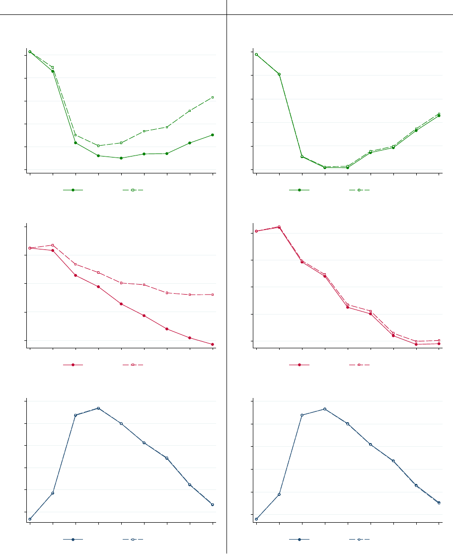
Figure A.1: The Age-Adjusted U.S. Employment Rate Decline

Ages 16+ Ages 25-54

A . Employment Rate D. Employment Rate

58 59 60 61 62 63

Employment rate (%)

2007 2008 2009 2010 2011 2012 2013 2014 2015

Unadjusted Age-adjusted

75 76 77 78 79 80

Employment rate (%)

2007 2008 2009 2010 2011 2012 2013 2014 2015

Unadjusted Age-adjusted

B. Labor Force Participation Rate E. Labor Force Participation Rate

63 64 65 66 67

Labor force participation rate (%)

2007 2008 2009 2010 2011 2012 2013 2014 2015

Unadjusted Age-adjusted

81 81.5 82 82.5 83

Labor force participation rate (%)

2007 2008 2009 2010 2011 2012 2013 2014 2015

Unadjusted Age-adjusted

C. Unemployment Rate F. Unemployment Rate

5 6 7 8 9 10

Unemployment rate (%)

2007 2008 2009 2010 2011 2012 2013 2014 2015

Unadjusted Age-adjusted

4 5 6 7 8 9

Unemployment rate (%)

2007 2008 2009 2010 2011 2012 2013 2014 2015

Unadjusted Age-adjusted

Notes: This ﬁgure uses monthly Current Population Surveys (CPS) to plot unadjusted and non-parametrically

age-adjusted annual U.S. employment rates (employment-population ratios), labor force participation rates,

and unemployment rates 2007-2015 for the civilian non-institutional population. The unadjusted statistics

are essentially equal to the oﬃcial Bureau of Labor Statistics U.S. labor force statistics. The age-adjusted

statistics reweight each age-year’s annual total unemployment, labor force, and population by the age group’s

2007 population share as in DiNardo, Fortin and Lemieux (1996) before summing across ages and computing

the displayed rates. See Online Appendix A for details.

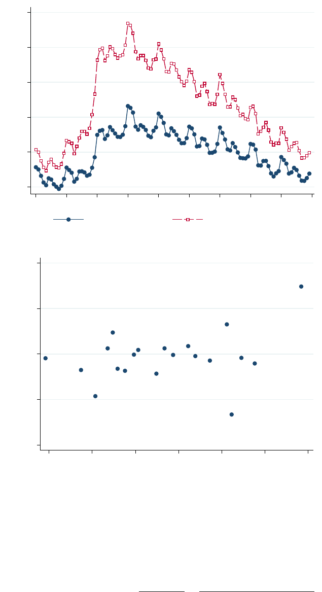
Figure A.2: Evidence against Positively Correlated Independent Shocks

A. Unemployment Rates by Shock Severity 2007-2015

4 6 8 10 12 14

Unemployment Rate (%)

2007 2008 2009 2010 2011 2012 2013 2014 2015 2016

Mildly shocked CZs Severly schocked CZs

B. 2010-2015 Shift-Share Shocks vs. Great Recession Local Shocks

15 16 17 18 19

2010-2015 shift-share shock (%)

2 3 4 5 6 7 8

Great Recession local shock (pp)

Notes: Panel A uses LAUS county-level data, aggregated to the CZ-level, to plot monthly mean unemployment

rates 2007-2015 in severely shocked CZs (those with above median Great Recession local shocks) and mildly

shocked CZs (all other CZs). Data points are weighted by CZ population. The post-2001-recession experience

exhibited incomplete convergence before being interrupted by positively correlated 2007-2009 shocks. Panel

B plots 2010-2015 CZ-level shift-share shocks versus Great Recession local shocks. The shift-share shocks are

constructed analogously to Bartik (1991) using County Business Patterns data as follows. Each CZ’s shift-share

shock equals the projected 2010-2015 percentage change in the CZ’s employment based on leave-one-CZ-out

nationwide changes in employment by three-digit NAICS industry categories. That is, a CZ c’s shift-share

shock equals: SHIF T SHARESHOCK



jc2010

c2010

6=c

2015

−

6=c

2010

6=c

2010



where j denotes a

three-digit industry and E

jct

denotes total employment in industry j in CZ c in year t. The graph bins CZs into

ventiles (ﬁve-percentile-point bins) by their Great Recession local shock and then plots the 2007-population-

weighted mean of the 2010-2015 shift share shock within each bin. If CZs that were severely shocked during

the Great Recession had subsequently experienced additional adverse shift-share shocks 2010-2015 related to

the CZs’ industrial compositions, Panel B would have exhibited a negative relationship instead of the displayed

insigniﬁcant positive relationship.

Figure A.3: Self-Employment vs. Formal Employment Rate Changes

-3.5 -3 -2.5 -2 -1.5 -1 -.5 0 .5

2015 self-employment rate minus

2007 self-employment rate (pp)

-6 -4 -2 0 2 4

2015 formal employment rate minus

2007 formal employment rate (pp)

Notes: This graph uses the 2007 and 2015 monthly Current Population Surveys to plot 2007-2015 self-

employment rate changes versus 2007-2015 formal employment rate changes for the adult (16+) civilian non-

institutionalized population. The formal employment rate equals the number of formally employed individuals

(workers for wages or salary in private or government sector) divided by the population. The self-employment

rate equals the number of self-employed individuals (including independent contractors) divided by the popu-

lation. Individuals are classiﬁed according to the job in which they worked the most hours. Each year’s rate

equals the monthly rate averaged across the year’s twelve months. Overlaid is the unweighted best-ﬁt line.

Figure A.4: State Employment Rate Persistence after 2007-2009 Shocks

A. Employment, Population, and B. Participation, Unemployment, and

Employment Rate after −1% Shock Employment Rates after −1% Shock

-2 -1.5 -1 -.5 0

Deviation from trend and aggregate

2007 2008 2009 2010 2011 2012 2013 2014 2015

Pred. employment (%) Act. employment (%)

Pred. population (%) Act. population (%)

Pred. employment rate (pp) Act. employment rate (pp)

-.5 -.25 0 .25 .5

Deviation from trend and aggregate

2007 2008 2009 2010 2011 2012 2013 2014 2015

Pred. unemployment rate (pp) Act. unemployment rate (pp)

Pred. participation rate (pp) Act. participation rate (pp)

Pred. employment rate (pp) Act. employment rate (pp)

C. Actual 2007-2014 Employment Rate

-.6 -.5 -.4 -.3 -.2 -.1 0

Deviation from trend and aggregate (pp)

2007

2008

2009

2010

2011

2012

2013

2014

2015

2016

2017

2018

2019

2020

2021

2022

2023

2024

Year relative to shock

Pred. based on 1978-1990 Pred. based on 1991-2007

Pred. based on 1978-2015 Actual 2007-2015

Notes: The dotted lines of panels A-B plot benchmark history-based predictions for state-level responses to

a −1% 2007-2009 state-level employment shock, based on estimating Blanchard-Katz’s (1992) autoregressive

system of state labor market outcomes using LAUS data on the original sample range 1978-1990. The solid

lines plot mean actual state-level responses based on reduced-form regressions of 2008-2014 state-level outcomes

on 2007-2009 state-level shocks. Panel C plots the mean actual employment rate response series from panels

A-B alongside predicted employment rate series based on three estimation time ranges: 1978-1990 (as in panels

A-B), 1991-2007, and 1978-2014. See Online Appendix B for more details.

Figure A.5: Great Recession Local Convergence Compared to History: Extended

A. Labor Force Participation Rate B. Unemployment Rate

-2 -1.5 -1 -.5 0 .5

Participation rate difference between severely

shocked and mildly shocked states (pp)

-5 -4 -3 -2 -1 0 1 2 3 4 5 6 7 8 9 10

Year relative to recession

1980-1982 recession

1990-1991 recession

2007-2009 recession

-.5 0 .5 1 1.5 2 2.5

Unemployment rate difference between severely

shocked and mildly shocked states (pp)

-5 -4 -3 -2 -1 0 1 2 3 4 5 6 7 8 9 10

Year relative to recession

1980-1982 recession

1990-1991 recession

2007-2009 recession

C. Employment Growth D. Population Growth

-8 -6 -4 -2 0

Employment growth: severely shocked states

minus mildly shocked states (log pts)

-5 -4 -3 -2 -1 0 1 2 3 4 5 6 7 8 9 10

Year relative to recession

1980-1982 recession

1990-1991 recession

2007-2009 recession

-5 -4 -3 -2 -1 0 1

Population growth: severely shocked states

minus mildly shocked states (log pts)

-5 -4 -3 -2 -1 0 1 2 3 4 5 6 7 8 9 10

Year relative to recession

1980-1982 recession

1990-1991 recession

2007-2009 recession

Notes: Panels A-B replicate Figure 2A for the labor force participation rate and unemployment rate. Panels

C-D display analogous graphs for employment growth and population growth. These latter panels require that

each state’s estimated steady state annual growth rate is subtracted from its actual annual growth, before

constructing the graphs exactly as in Panels A-B. See Online Appendix B and the notes to Figure 2.

Outcome:

Individual-level 2015 relative

employment (from tax data)

CZ-level estimated employment

effect (from tax data)

CZ-level 2015 relative employment

(from BLS LAUS and Census)

(pp) (pp) (pp)

(1) (2) (3)

Great Recession local shock

-0.393 -0.381 -0.490

(0.097) (0.100) (0.115)

Main controls

Main sample (individual-level)

Published sample (CZ-level)

X X

1,357,974 591 591

0.07 0.10 0.09

ONLINE APPENDIX TABLE 1

Approximating the Main Result Using Published Data

Notes – This table shows that the paper's main estimate of the 2015 employment impact of Great Recession local shocks—which uses the main

sample's non-public individual-level data—can be well-approximated in CZ-level data published alongside this paper. Column 1 reprints the main

specification and estimate from Table 2 column 4. Columns 2-3 report coefficients from univariate CZ-level regressions weighted by the CZ's 2007

population as reported in Census's Annual County Resident Population Estimates of the total adult (16+) population, aggregated to the CZ level. The

column 2 outcome equals the estiamated coefficients on a vector of CZ fixed effects from estimating the main specification with Great Recession local

shock variable replaced by a vector of CZ fixed effects. Online Appendix Table 2 lists these estimated coefficients for the hundred largest CZs. The

column 3 outcome variable equals the CZ's 2015 adult employment rate minus the CZ's mean 1999-2007 employment rate, based on Census data and

Bureau of Labor Statistics Local Area Unemployment Statistics data: LAUS county-level 16+ civilian non-institutional employment aggregated to the CZ

level, divided by Census's CZ population estimate. Column 3 is restricted to the CZs available for column 2. Standard errors are clustered in column 1

by the individual's 2007 state and in columns 2-3 by the CZ's state. See the paper's Online Data Codebook and Online Data Tables for additional

details and published variables on the author's website.

Outcome (relative or

absolute):

Employed

Migrated

outside 2000

Employed in

2000 CZ

Employed

outside 2000

Earnings

Earnings in

2000 CZ

Earnings

outside 2000

UI income SSDI income

(pp) (pp) (pp) (pp) ($) ($) ($) ($) ($)

(1) (2) (3) (4) (5) (6) (7) (8) (9)

Effect in 2000

-0.036 0.000 -0.036 0.000 72 72 0 0.6 0.4

(0.083) (0.083) (66) (66) (6.2) (3.9)

Effect in 2001

-0.094 -0.036 -0.093 -0.001 -74 -67 -7 10.6 0.3

(0.045) (0.166) (0.044) (0.003) (46) (42) (6) (9.2) (4.6)

Effect in 2002

-0.068 -0.047 -0.060 -0.008 -56 -47 -9 9.7 0.7

(0.018) (0.280) (0.017) (0.004) (26) (23) (5) (15.4) (5.4)

Effect in 2003

-0.044 -0.005 -0.036 -0.008 -26 -17 -10 10.2 0.6

(0.029) (0.361) (0.031) (0.007) (21) (20) (6) (15.9) (5.8)

Effect in 2004

0.031 0.077 0.030 0.001 1 6 -5 11.0 0.3

(0.039) (0.437) (0.036) (0.009) (36) (30) (12) (11.9) (6.6)

Effect in 2005

0.083 0.151 0.070 0.013 40 42 -1 6.8 -0.1

(0.061) (0.526) (0.053) (0.010) (66) (57) (22) (11.5) (7.3)

Effect in 2006

0.228 0.252 0.189 0.039 -15 1 -16 9.1 0.4

(0.135) (0.612) (0.116) (0.020) (118) (94) (36) (13.1) (9.1)

ONLINE APPENDIX TABLE 2

Adjustment Margins Pre-Trends

Notes – This table replicates Table 5 for years 2000-2006 and where each individual's Great Recession local shock equals the 2007-2009 percentage-point unemployment

rate change in the individual's 2000 CZ. See the notes to Table 5 for details.

Mean Standard Deviation

(1) (2)

Employment rate (%)

1978-2015 62.3 4.6

2007 64.1 3.9

2009 60.7 4.5

2015 60.4 4.4

Unemployment rate (%)

1978-2015 6.1 2.1

2007 4.4 1.0

2009 8.5 2.0

2015 5.0 1.1

Labor force participation rate (%)

1978-2015 66.3 4.1

2007 67.0 3.8

2009 66.3 4.0

2015 63.6 4.1

Number of states

Number of years

Number of observations (state-years)

Notes – This table lists summary statistics of the Bureau of Labor Statistics's Local Area

Unemployment Statistics (LAUS) state-year labor force statistics 1978-2015. The LAUS data cover

the adult (16+) civilian non-institutional population of the fifty states and the District of Columbia.

The employment rate is the ratio of employment to population. The unemployment rate is the ratio

of unemployed to labor force. The labor force participation rate is the ratio of labor force to

population.

ONLINE APPENDIX TABLE 3

Summary Statistics: State-Level Data

1,938

Great

Recession

Employment

Shock Rank

State

Great

Recession

Employment

Shock

Change in

Employment

Rate

2007-2015

Great

Recession

Employment

Shock Rank

State

Great

Recession

Employment

Shock

Change in

Employment

Rate

2007-2015

(pp) (pp) (pp) (pp)

(1) (2) (3) (4) (5) (6) (7) (8)

1 Nevada -6.46 -6.94 27 Washington 1.13 -5.21

2 Alabama -3.42 -5.54 28 New Hampshire 1.13 -2.03

3 Michigan -3.36 -2.74 29 Missouri 1.24 -1.42

4 Georgia -3.19 -7.09 30 Arkansas 1.26 -4.79

5 Delaware -3.14 -4.65 31 Texas 1.30 -2.06

6 Mississippi -3.04 -4.21 32 Virginia 1.56 -4.87

7 Utah -2.53 -4.31 33 Maryland 1.92 -2.79

8 Florida -2.40 -5.45 34 Louisiana 1.99 -2.41

9 South Carolina -2.35 -3.59 35 Massachusetts 2.06 -1.64

10 Arizona -2.24 -4.82 36 Alaska 2.26 -3.67

11 Idaho -2.20 -4.53 37 Minnesota 2.33 -2.24

12 North Carolina -2.15 -4.79 38 New Jersey 2.37 -3.21

13 Tennessee -1.56 -5.18 39 West Virginia 2.58 -4.18

14 Indiana -1.52 -2.45 40 Pennsylvania 2.68 -2.15

15 Hawaii -1.33 -4.27 41 New York 2.79 -2.28

16 Oregon -1.29 -4.33 42 Oklahoma 3.25 -1.90

17 California -0.63 -3.74 43 Connecticut 3.33 -3.33

18 New Mexico -0.57 -6.80 44 South Dakota 3.56 -3.98

19 Illinois -0.33 -4.02 45 Wyoming 3.85 -4.30

20 Ohio 0.05 -4.19 46 Kansas 4.35 -2.98

21 Montana 0.46 -3.45 47 Vermont 4.38 -2.93

22 Colorado 0.73 -5.15 48 Nebraska 4.77 -2.99

23 Wisconsin 0.75 -2.48 49 Iowa 5.00 -2.03

24 Rhode Island 0.81 -3.98 50 District of Columbia 5.44 0.94

25 Kentucky 0.90 -4.60 51 North Dakota 5.75 -2.48

26 Maine 1.09 -3.39

ONLINE APPENDIX TABLE 4

State-Level Great Recession Employment Shocks and 2007-2015 Employment Rate Changes

Notes – This table lists the Great Recession state-level employment shocks and 2007-2015 percentage-point changes in state-level employment

rates that underlie the severe-vs-mild-shock grouping of Figure 1B. See the notes to those figures and Online Appendix B for details. Severely

shocked states are listed on the left; mildly shocked states are listed on the right.

Outcome relative to pre-2007 mean:

(pp) (pp) (pp) (pp) (pp) (pp) (pp) (pp)

(1) (2) (3) (4) (5) (6) (7) (8)

Great Recession local shock -0.393 -0.375 -0.393 -0.393 -0.393 -0.393 -0.369 -0.366

(0.097) (0.107) (0.082) (0.100) (0.092) (0.094) (0.097) (0.097)

Main controls X X X X X X X X

Locally deflating earnings in fixed effects X

CZ has valid Hispanic share 2009-2015 X X

Change in Hispanic share 2009-2015 X

Clustering on 2007 state and 2006 industry X

Clustering on 2007 state and age X

Clustering on 2007 state and 2006 earnings bin X

Clustering on 2007 state and 2006-age- X

earnings-industry

N 1,357,974 1,357,974 1,357,974 1,357,974 1,357,974 1,357,974 1,271,391 1,271,391

0.07 0.08 0.06 0.06 0.06 0.06 0.08 0.08

Notes – Column 1 reprints the paper's main estimate from Table 2 column 4. Column 2 uses locally deflated 2006 earnings when constructing the 2006-age-

earnings-industry fixed effects. Columns 3-4 two-way cluster on the listed variables. Column 7 repeats column 1 for the individuals whose 2007 CZs have a non-

missing Hispanic share in 2009 and 2015 in the American Community Survey. Column 8 controls for the individual's 2007 CZ's 2015 Hispanic share minus that

CZ's 2009 Hispanic share.

Employed in 2015

LETTER TABLE 1

Specifications for Referee Responses

Effect Rank CZ Name

Estimated

Employment

Effect

Effect Rank CZ Name

Estimated

Employment

Effect

(pp) (pp)

(1) (2) (3) (5) (6) (7)

Fayetteville, NC -4.11 51 Cincinnati, OH 0.14

2 Albuquerque, NM -3.95 52 Portland, OR 0.15

3 Deltona, FL -2.97 53 Grand Rapids, MI 0.19

4 Pensacola, FL -2.88 54 Charlotte, NC 0.26

5 Bakersfield, CA -2.46 55 San Jose, CA 0.28

6 Jacksonville, FL -2.45 56 Columbus, OH 0.28

7 Birmingham, AL -2.43 57 Harrisburg, PA 0.28

8 Little Rock, AR -2.30 58 Los Angeles, CA 0.30

9 Toledo, OH -2.26 59 Rockford, IL 0.30

10 Lakeland, FL -2.13 60 Atlanta, GA 0.32

11 Greenville, SC -2.12 61 Allentown, PA 0.34

12 Sarasota, FL -1.92 62 Canton, OH 0.37

13 Las Vegas, NV -1.86 63 Erie, PA 0.40

14 Baton Rouge, LA -1.83 64 Indianapolis, IN 0.41

15 Palm Bay, FL -1.77 65 Albany, NY 0.41

16 Eugene, OR -1.62 66 Louisville, KY 0.45

17 Tampa, FL -1.39 67 Newark, NJ 0.51

18 Knoxville, TN -1.37 68 Toms River, NJ 0.51

19 Columbia, SC -1.26 69 Cleveland, OH 0.52

20 Modesto, CA -1.24 70 Santa Barbara, CA 0.52

21 Tulsa, OK -1.23 71 Raleigh, NC 0.53

22 Fresno, CA -1.23 72 Bridgeport, CT 0.55

23 Tucson, AZ -1.04 73 San Diego, CA 0.58

24 Charleston, SC -1.02 74 Washington, DC 0.58

25 New Orleans, LA -0.98 75 Buffalo, NY 0.59

Sacramento, CA -0.93

Kansas City, MO 0.61

Phoenix, AZ -0.90

San Antonio, TX 0.66

Nashville, TN -0.89

Poughkeepsie, NY 0.67

San Francisco, CA -0.80

South Bend, IN 0.75

Oklahoma City, OK -0.80

Syracuse, NY 0.82

St. Louis, MO -0.80

Scranton, PA 0.83

Virginia Beach, VA -0.78

New York, NY 0.91

Memphis, TN -0.74

Austin, TX 1.12

Dayton, OH -0.67

Fort Worth, TX 1.13

Greensboro, NC -0.64

Chicago, IL 1.28

Detroit, MI -0.59

Milwaukee, WI 1.29

Richmond, VA -0.47

Pittsburgh, PA 1.42

Portland, ME -0.41

Manchester, NH 1.43

Providence, RI -0.26

Madison, WI 1.46

Youngstown, OH -0.22

Houston, TX 1.55

Spokane, WA -0.14

Boston, MA 1.70

Seattle, WA -0.10

Dallas, TX 1.78

Gary, IN 0.02

Des Moines, IA 1.79

Cape Coral, FL 0.02

Reading, PA 1.93

Orlando, FL 0.04

Miami, FL 1.94

Baltimore, MD 0.04

Minneapolis, MN 2.14

Springfield, MA 0.06

El Paso, TX 2.58

Port St. Lucie, FL 0.09

Salt Lake City, UT 2.61

Denver, CO 0.10

Omaha, NE 2.98

Philadelphia, PA 0.13

100

Brownsville, TX 5.47

ONLINE APPENDIX TABLE 2

Estimated Employment Effects for the 100 Largest Commuting Zones

Notes - This table lists estimated effects of living in 2007 in each of the hundred largest CZs on 2015 employment, drawn

from the complete data published online. The paper's main specification (Table 2 column 4) regresses 2015 relative

employment (2015 employment minus mean 1999-2006 employment) on Great Recession local shocks and 2006-age-

earnings-industry fixed effects. To generate this table, I repeat the main specification except that I replace the Great

Recession local shock variable with a vector of CZ fixed effects. I then de-mean the 2007-population-weighted fixed

effects and list the fixed effects of the hundred largest CZ's by 2007 population. 2007 population is drawn from Census's

Annual County Resident Population Estimates of the total 16+ population aggregated to the CZ level. See Online Data

Table 1 on the author's website for the full list of CZ-level effects and other CZ-level statistics. Online Appendix Table 1

column 2 shows that the published CZ-level data can be used to approximate the paper's main individual-level regression

result.