Distributional National Accounts: Methods and Estimates for the United States

NBER WORKING PAPER SERIES

DISTRIBUTIONAL NATIONAL ACCOUNTS:

METHODS AND ESTIMATES FOR THE UNITED STATES

Thomas Piketty

Emmanuel Saez

Gabriel Zucman

Working Paper 22945

http://www.nber.org/papers/w22945

NATIONAL BUREAU OF ECONOMIC RESEARCH

1050 Massachusetts Avenue

Cambridge, MA 02138

December 2016

We thank Tony Atkinson, Oded Galor, David Johnson, Arthur Kennickell, Jean-Laurent

Rosenthal, John Sabelhaus, David Splinter, and numerous seminar and conference participants

for helpful discussions and comments. Antoine Arnoud, Kaveh Danesh, Sam Karlin, Juliana

Londono-Velez, Carl McPherson provided outstanding research assistance. We acknowledge

financial support from the Center for Equitable Growth at UC Berkeley, the Institute for New

Economic Thinking, the Laura and John Arnold foundation, NSF grant SES-1559014, the Russell

Sage foundation, the Sandler foundation, and the European Research Council under the European

Union's Seventh Framework Programme, ERC Grant Agreement No. 340831. The views

expressed herein are those of the authors and do not necessarily reflect the views of the National

Bureau of Economic Research.

NBER working papers are circulated for discussion and comment purposes. They have not been

peer-reviewed or been subject to the review by the NBER Board of Directors that accompanies

official NBER publications.

sections of text, not to exceed two paragraphs, may be quoted without explicit permission

provided that full credit, including © notice, is given to the source.

Distributional National Accounts: Methods and Estimates for the United States

Thomas Piketty, Emmanuel Saez, and Gabriel Zucman

NBER Working Paper No. 22945

December 2016

JEL No. E01,H2,H5,J3

ABSTRACT

This paper combines tax, survey, and national accounts data to estimate the distribution of

national income in the United States since 1913. Our distributional national accounts capture

100% of national income, allowing us to compute growth rates for each quantile of the income

distribution consistent with macroeconomic growth. We estimate the distribution of both pre-tax

and post-tax income, making it possible to provide a comprehensive view of how government

redistribution affects inequality. Average pre-tax national income per adult has increased 60%

since 1980, but we find that it has stagnated for the bottom 50% of the distribution at about

$16,000 a year. The pre-tax income of the middle class—adults between the median and the 90th

percentile—has grown 40% since 1980, faster than what tax and survey data suggest, due in

particular to the rise of tax-exempt fringe benefits. Income has boomed at the top: in 1980, top

1% adults earned on average 27 times more than bottom 50% adults, while they earn 81 times

more today. The upsurge of top incomes was first a labor income phenomenon but has mostly

been a capital income phenomenon since 2000. The government has offset only a small fraction

of the increase in inequality. The reduction of the gender gap in earnings has mitigated the

increase in inequality among adults. The share of women, however, falls steeply as one moves up

the labor income distribution, and is only 11% in the top 0.1% today.

Thomas Piketty

Paris School of Economics

48 Boulevard Jourdan

75014 Paris, France

[email protected]

Emmanuel Saez

Department of Economics

University of California, Berkeley

530 Evans Hall #3880

Berkeley, CA 94720

and NBER

[email protected]

Gabriel Zucman

Department of Economics

University of California, Berkeley

530 Evans Hall, #3880

Berkeley, CA 94720

and NBER

[email protected]

1 Introducti on

Income inequality has i n cr ea sed in many developed countries over the last se veral decades.

This trend has attrac te d considerable interest among academics, polic y- m akers, and the gen er a l

public. In recent years, followin g up on Kuznets’ (1953) pioneering attempt, a number of authors

have used administrative tax records to construct long-run series of top income shares (Alvaredo

et al., 2011-2016). Yet despite this endeavor, we still face three importa nt l i m i t at i o n s when

measuring income inequality. First and most importa nt, there is a larg e gap between nation al

accounts— wh i ch focus on macro totals and growth—and inequality studies—which focus on

distributions using survey and t a x data, usu al l y without trying to be ful l y consistent with

macro totals. This gap makes it hard to address questions such as: What fraction of economic

growth accrues to the bo t t om 50%, the middle 40%, and the top 10% of the distribution? How

much of the rise in income inequality owes to changes in the share of labo r and capital in national

income, and how much to changes in the dispersion of labor earni n gs , capital ownership, and

returns to capital? Second, about a third of U.S. national income is redistributed through taxes,

transfers, and public good spending . Yet we do not have a good measure of how the distribution

of pre-ta x income diﬀers from the distribution of po st -t a x income, mak i n g it hard to assess how

government redi st ri b u t i o n aﬀects inequality. Th i rd , existing income inequality st a t i st i cs use the

tax unit or the household as unit of observation, ad d i n g up t h e i n co m e of men an d women. As a

result, we do not have a clea r vi ew of how long-run trends in income concentration are shaped by

the major changes in women labor force participation—and gender inequality general l y— th a t

have occurred over the last century.

This paper attempts to compute ineq u a l i ty statistics for the United States that overcome the

limits of existing series by creating distributional national accounts. We combine tax, survey,

and n a t i on a l accounts data to bui l d new series on the distribution of national inc om e since

1913. In contrast to previo u s attempts that capture less than 60% of US n at i on a l income—

such as Census bureau estimates (US Census Bureau 2016) and top income shares (Piketty

and Saez, 2003)—our estimates capture 100% of the nati o n al income recorded in the natio n a l

accounts. This enables us to provide decomposit i o n s of growth by income groups consistent

with macroeconomic growth. We co m p u t e the distribution of both pre-tax and post -t ax income.

Post-tax series deduct all tax es and add back all transfers and publi c spending, so that both

pre-tax and post-tax in co m es add up to national incom e. This al l ows us to provide the ﬁrst

comprehensive view of how government redistribution aﬀects inequality. Our benchmark series

uses the adult individual as the unit of obser vation and splits in co me eq u al l y a m o n g spouses.

We also rep o r t series in which each spous e is assigned her or his own labor income, enabling us

to study how long-run changes in gender inequality shape the distribution of i n co m e.

Distributional nation al accounts provide information on the dynamic of income acro ss the

entire spectrum—from the bottom decile to the top 0. 00 1% — th a t , we believe, is more accurate

than existing inequality data. Our estimates capture employee fringe beneﬁts, a growin g source

of income for the middle-class that is overlooked by both Census bureau estimates and tax

data. They capture all capital income, which is large—about 30% of total national income—

and concentrated, yet is very imperfectly covered by surveys—due to small sample and top

coding issues—and by tax data—as a large fraction of capit a l income g oes to pension funds and

is re ta i n ed in corporations. They make it possible to produce long-run inequality statistics that

control for socio-demographic changes—such as the rise in the fraction of retired individuals

and the decline in household size—contrary to the currently available tax-based series.

Methodologically, our contribution is to construct mic ro -ﬁ l e s of pre-tax and post-tax income

consistent with macro aggregates. These micro-ﬁles contain all the variables of the national

accounts and synthetic individ u a l observations that we obtain by statistical l y match i n g tax

and survey data and making explicit assumptions about the distribution of income categories

for whi ch there is no directly available source of i n fo r m at i o n . By construction, the t o t al s in

these micro-ﬁles add up to the national accounts totals, while the distributions are consistent

with those seen in tax and survey d a t a. These ﬁles can be used to compute a wide array

of distributional statistics—labor and capi ta l i n co m e earne d , taxes paid, transfer s rece i ved,

wealth owned, etc. —by age groups, gender, and marital status. Our objective, in the years

ahead, is to c on st r u ct similar micro-ﬁles in as many countries as possible in order to better

compare inequality across countries.

Just like we u se GDP or national income to compare the

macroeconomic performances of countries today, so coul d distributional national accounts be

used to compare ineq u a l i ty across countries tomorrow.

We stress at the outset that there are numerous data issues involved in distributing national

income, discussed in the text and the online appendix.

First, we take the national accou nts

as a given sta rti n g point, although we a r e well aware that the national accounts themsel ves are

imperfect (e. g. , Zucman 2013). They are, however, the most reasona b l e starting point, because

they aggregate all the available information from surveys, tax data, corporate income state-

All updated ﬁles and results will be made available on-line on the World Wealth an d Income Database

(WID.world) website: http://www.wid.world/. All the US results and data are also posted at http:

//gabriel-zucman.eu/usdina/.

The online appendix is available at http://gabriel-zucman.eu/files/PSZ2016DataAppendix.pdf.

ments, and balance sheets, etc., in an standardized, internationally-agr eed -u pon and regularly

improved upon accounting framework. Secon d , impu t i n g all national income, taxes, transfers,

and public goods spending requires making assumptions on a number of complex issues, such as

the economic incidence of taxes and who beneﬁts from government spending. Our goal is not to

provid e deﬁniti ve answers to these questions, but rather to be comprehensive, consist ent, and

explicit about what assumptions we are making and why. We view our paper as attempting to

construct prototyp e distributional national accounts, a pr ot o type that could be improved upon

as more dat a become available, new knowledge emerges on who pays t ax es and beneﬁts from

government spend i n g , an d reﬁned estimat i o n techniques are developed—just as today’s national

accounts are regularly improved.

The analysis of our US distributional national acco u nts yield s a number of striking ﬁndings.

First, our data show a sharp diverge n ce in the growth experienced by the bottom 50% versus

the rest of th e economy. The average pre-tax income of the bottom 50% of adults has stagnated

since 1980 at a bout $16,000 per adult (i n constant 2014 dollars, using the national income

deﬂator), while average national income per adult has grown by 60% to $64,500 in 2014. As a

result, the bottom 50% income share has coll ap se d from about 20% in 1980 to 12% in 2014. In

the meantime, the average pre-tax income of top 1% adu l ts rose from $420,000 to about $1.3

million, and their income share increa sed from about 12% in the early 1980s to 20% in 2014.

The two gr o u p s have essential l y switched their income shares, with 8 points of national income

transferred from the bottom 50 % to the top 1%. The top 1% income shar e is now almost twice

as lar g e as the bottom 50% s h are, a group th a t is by deﬁnition 50 t i m es more numerous. In

1980, top 1% adults earned on average 27 times more than bottom 50% adults before tax while

today they earn 81 times more.

Second, gover n m ent redistribut i on has o ﬀse t only a small fraction of the increase in pre-tax

inequality. Even after taxes and transfe rs , there has been close to zero growth for working-age

adults in the bottom 50% of the distribution since 1980. The aggregate ﬂow of individualized

government transfers ha s increased, but these transfers are largely targeted to the elderly and

the middle-class (individuals above the me d i an and below the 90th percentile). Transfers that

go to the bottom 50% have not been large enough to lift income signiﬁcantly. Given the massive

changes in the pre-tax di st r i b u t i on of natio n a l income si n ce 1980, there are clear limits to what

redistributive policies can achieve. In light of the collapse of bottom 50% primary incomes,

we feel th a t policy discussions should focus on how to equalize the distribution of p r i m a ry

assets, including human capital, ﬁnancial capital, and bargaining power, rather than merely

ex-post redistribution. Poli ci es that could raise bottom 50% pre-tax incomes include improved

education and access to skills, which may r eq u i re major changes in the system of education

ﬁnance and admission; reforms of l a bo r m a rket institutions, in cl u d i n g minimu m wage, corporate

governance, and wo r ker co-determination; and steeply progressive taxation, which can aﬀect pay

determination and pre-tax distr i b u t i on , particularly at the top end (see, e.g., Piketty, Saez and

Stantcheva 2014, and Piketty 2014).

Third, we ﬁnd that the upsurge of top incomes has mostly been a capital- d r i ven phenomenon

since the lat e 1990s. There is a widespread view that rising income inequ al i ty most ly owes to

booming wages at the top end, i.e., a rise of the “wor k i n g rich.” Our results conﬁrm that this

view is correct from the 1970s to the 1990s. But in contra st to earlier decades, the increase in

income concentration over the last ﬁfteen years owes to a boom in the in com e from equity and

bonds at the top. The working rich are either turning into or bei n g replaced by rent i er s. Top

earners became younger in the 1980s and 1990s but have been growing older since then.

Fourth, the r ed u c ti o n in the gender gap has mitigated the increase in inequality among

adults since the la te 1960s, but the United States is still characterized by a spectacular glass

ceiling. When we allocate labor incomes to indivi d u a l earners (instead of splitting it equally

within couples , as we do in our benchmark series), the rise in inequality is less drama tic , than k s

to the rise of female labor market participation. Men aged 20-64 earned on average 3.7 times

more labor income than women aged 20-64 i n the early 1960s, while they earn 1.7 times more

today. Until the early 1980s, the top 10%, top 1%, and top 0.1% of the labor income distribution

were less than 10% women. Since then, this share has increased, but the increase is smaller the

higher one moves up in the distrib u t i on . As of 2014, women make only about 16% of the top

1% lab o r income earners, and 11% of the top 0.1%.

The paper is organized as fol l ows. Section 2 relates our work to the existing literature.

Section 3 lays out our methodology. In Section 4, we present our results on the distribution

of pre-tax and post-tax national income, and we provide decompositions of growth by income

groups consistent with macroeconomic growth. Sectio n 5 analyze s the role of changes in gender

inequality, factor shares, and taxes and transfers for the dynamic of US i n co m e inequality. S ec-

tion 6 compa r es and reconciles our r esu l t s with previous estimates of US income con centration.

We conclude in Secti on 7.

2 Previous Attempts at Introducing Distributional Mea-

sures in the National Accounts

There is a long tradition of research attempting to introdu ce distributional measures in the

national accounts. The ﬁrst national accounts in history—the famou s social tables of King

produced in the late 17th century—were in fact distributional national accounts, showing the

distribution of England’s income, consump t i o n , and saving across 26 social classes—from tem-

poral lords and baronets down to vagrants—in the year 1688 (see Barnet t , 1936). In the Uni t ed

States, Kuz n et s was interested in both national income and i ts distribut i o n and made path-

breaking advances on both fronts (Kuznets 1941, 19 53 ) .

His innovation wa s estimating top

income shares by combining tabulations of federal income tax returns—from wh i ch he derived

the income o f top earners using Pareto extrapolations—and newly constructed national accounts

series—that he used to compute the total incom e denominato r. Kuznets, however, did not fully

integra t e the two approa ches: his inequality series capture taxable income only and mis s all

tax-exempt cap i t al and labor income. The top income shares later computed by Piketty (2001,

2003), Piketty and Saez (2003), Atkinson (2005) and Alvaredo et al. (2011-2016) extended

Kuznets’ methodology to more countries and years but did not address this shortcoming.

Introdu ci n g distri b u t i on a l measures in the national accounts has received ren e wed i nterest

in recent years. In 2009, a report from the Commission on the Measurement of Economic Per-

formance an d Social Progress emphasized the impor t an c e of incl u d i n g distributional measures

such as household income quintiles in the Sy st em of National Account s (Stiglitz, Sen and Fi-

toussi, 2009). In response to th i s report, a number of countries, su ch as Australia, introduced

distributional statistics in their national accounts (Australian Bureau of Statistic, 2013) while

others are i n the process of doing so. Furlong (2014), Fixler and Johnson (2014), McCully

(2014), and Fixler et al. (2015) describe the ongoing U.S. eﬀort, which focuses on scaling u p

income from the Cur re nt Population Survey to match personal income.

There are two main methodological diﬀerences between our paper and the work currently

conducted by statistical agencies. Fi r st , we start with tax data—rather than surveys—that we

supplement with surveys to capture forms of income that are not visible in tax returns, s u ch

as tax-exempt transfers. The use of tax data is critical to capture the to p of the d i st ri b u t i o n ,

Earlier attempts include King (1915, 1927, 1930).

Using tax data, Auten and Splinter (2016) have recently produced US income conc entration stati s t ic s since

1962 that improve upon the Piketty and Saez ( 2003) ﬁscal income series by distributing total personal income

(instead of total pre-tax and post-tax national income as we do here) from the national accounts. We view their

work as complementary to ou rs .

which ca n n ot be studied properly with s u rveys becau s e o f top-coding, insu ﬃ ci e nt over-sampling

of the top, sampling errors, or non-sam p l i n g errors.

Second, we are primarily inte re st ed in

the distribution of total n at i o n al income rather than household or personal income. National

income is in our view a m o r e meaningful starting point, because it is interna t i on a l l y comparable,

it is the aggregate used to comp u t e macroeconom i c growth, and it i s comprehensi ve, including

all forms of in co m e that eventually accrue to in d i v i d u a l s.

While we focus on national income,

our micro-ﬁles can be used to st u d y a wide range of income concepts, i n cl u d i n g the household

or perso n a l income concepts more traditionally analyzed.

Little work has contrasted the distributio n of pre-tax income with that of post -t ax income.

Top income sha r e studies only deal with pre-tax income, as many forms of transfers are tax-

exempt. Oﬃcial income st a ti s ti c s fr om the Census Bureau focus on pre-tax income and include

only some government transfers (US Census Bureau 2016).

Congressional Bu d g et Oﬃce esti-

mates compute both pre-tax and post-tax inequality measures, but they include only Federal

taxes and do not try to incorporate government consumption (US Congressional Budget Oﬃce

2016). By contrast, we at t em pt to allocate all taxes (in cl u d i n g State and local taxes) and all

forms of government spending in order to provide a comprehensive view of how government

redistribution aﬀects inequality.

Last, there is a large and growing theoretical literature jointly analyzing economic growth

and income dist ri b u t i o n . Historically, the Kuznets curve theory of how inequality evolves over

the path of development ( Ku zn e ts , 1955) came out of the seminal empirical work by Kuznets

(1953) on US incom e inequality. We hope that our estimates will similarly be fruitful to stimulate

future theoretical work on the interplay between growth and inequality.

Another possibil i ty would be to use the CPS as the baseline dataset and supplement it with tax data for the

top decile, where the CPS suﬀers from small samples, poorly measured capital income, and top-coding issues.

The advantage of starting from the CPS would b e that it has been the most widely known and used dataset to

analyze US income and wage inequality for many decades. We leave this alternative approach to future work.

Per son al income is a concept that is speciﬁc to the U.S . National Income and Product Accounts (NIPA).

It is an ambiguous concept (neither pre-tax, nor post-tax), as it does not deduct taxes but adds back cash

government transfers. The System of National Accounts (United Nations, 2009) does not us e personal income.

In our v i ew, not deducti n g taxes but counting (some) transfers is not conceptually meaningful, but it parallels

the deﬁnition of personal income in the US national accounts.

In recent decades, a lot of the work on inequality and growth has focused on the role of credit constraints

and wealth inequality (see, e.g., Galor and Zeira, 1992). Our data jointly capture wealth, capital income, and

labor income, making it possible to cast light on this debate and to study changes in the structure of inequality,

e.g., the extent to w hi ch there has truly been a demise of the capitalists-workers class structure (Galor and Moav

2006).

3 Methodolo gy to Distribute US N a ti ona l Income

In this section, we outline the main concepts and methodology we use to distribute US national

income. All the data sou r ce s and computer code we use are described in Online Appendix A;

here we focus on the main conceptual issues.

3.1 The Income Concept We Use: National Income

We are interested in the distribution of total national income. We fo l l ow the oﬃcial deﬁnition of

national income codiﬁed in the latest System of National Accounts (SNA, United Nati on s, 2009),

as we do for all other national accounts concepts used in this paper. National i n co m e is GD P

minus capital dep r eci a t i on plus net income recei ved from abroad. Although macroeconomists,

the press, and the general public often focus on GDP, na t i on a l income is a more meaningful

starting point for two re aso n s. First, capital depreciation is not economic incom e: it does

not allow one to consume or accumulate wealth. Allocating depreciation to individuals woul d

artiﬁcially inﬂate the economic income of capital owners. Second, including foreign income is

important, because for ei gn dividends and interest are sizable f or top earners.

In moving away

from GDP and toward national income, we follow one of the recommendations m ad e by the

Stiglitz, Sen and Fitoussi (2009) commission and also return to the pre-World War II focus on

national income (King 1930, Kuzne ts , 1941).

The national income of the United States is the sum of all the labor i n co m e—t h e ﬂow return

to human capital—and capital income—the ﬂow ret u r n to non-human capital—that accrues

to U.S. resident individuals. Some parts of national income never show up on any person’s

bank account, but it is not a reason to ignore them. Two prominent examples are the imputed

rents of homeowners and taxes. First, there is an economic return to owning a house, whether

the house is rented or not; national income therefore includes bot h monetary rents—for houses

rented out —a n d im p u t ed rents—for owner-o ccu p i e rs . Secon d , some income is immediately pai d

to the government in the form of payroll or corporate ta x es, so that no individual ever feels it

A discussion of the general issues involved in creating distributional national accounts is presented in Al-

varedo et al. (2016). These guidelines are not speciﬁc to the United States but they are based on the lessons

learned from constructing the US distribut i on al national accounts presented here, and from similar on-going

projec t s in other countries.

National income also includes the sizable ﬂow of undistributed proﬁts reinvested in foreign companies that

are more than 10% U.S.-owned (hence are class i ﬁe d as U.S. d ir e ct investments abroad). It does not, however,

include undistributed proﬁts reinvested in foreign companies in which the U.S. owns a share of less than 10%

(classiﬁed as portfolio investments). Symme tr i cal l y, national income deducts all t h e primary income paid by the

U.S. to non-residents, including the undistributed proﬁts reinvested in U.S. companies that are more than 10%

foreign-owned.

earns th a t fractio n of national income. But these taxes are part of the ﬂow return to capital and

labor and as such accrue to the owners of the factors of production. The same is true for sales

and excise taxes. Out of their sales proceeds at market prices (including sales taxes), producers

pay workers labor income and owners cap i t al income but must also pay sales and excise taxes to

the government. Hence, sales and excise taxes are part of national income even if they are not

explicitly part of employee compensation or proﬁts. Who exactly earns the fraction of nationa l

income pai d in the form of corporate, payroll, and sales taxes is a tax in ci d en c e question to

which we return in Secti on 3.3 bel ow. Although national income inclu d es all th e ﬂow retur n

to the factors of production , it does not include the ch a n g e in the price of these factors; i.e., it

excludes the capital gains caused by pure asset price changes.

National in co m e is larger an d has been g r owing faster than the other income concepts tr ad i -

tionally used to study in eq u al i ty. Figure 1 provides a reconciliation betwe en national income—as

recorded in the national accounts—a n d the ﬁscal income reported by ind i v i d u a l taxpayers to the

IRS, for labor and capital income separately.

About 70% of national income is labor income

and 30% is capital income. Although most of national labor income is reported on tax returns

today, the gap between taxable labor income and national labor income has been growing over

the last several decades. Untaxed l a bor income includes tax-exempt fringe beneﬁts, employer

payrol l taxes, the labor income of non ﬁlers (large before the early 1940 s) and unreported labor

income due to tax evasion. The fraction of labor income which is taxable has declined from 80%-

85% in the post-Wor l d War II decades to just under 70% in 2014, due to the rise of employee

fringe beneﬁts. As for capital, on l y a third of total capital income is reported on tax returns.

In addition to the imp u t ed rents of homeowners and various taxes, untaxed capital income in-

cludes the di v i d end s and interest paid to tax-exempt pension accounts, and corporate retained

earnings. The l ow ratio of taxable to t ot a l capital income is not a new p h en o m eno n —t h er e is no

trend in this ratio over time. However, when taking into account both labor and capital incom e,

the fraction of national income that is reported in individual income tax da t a has declined from

70% in the late 1970s to about 60% today. This result implies that tax data un d er -e stimate

In the long-run, a large fraction of capit al gains arises fr om the fact that corporations retain part of their

earning, which leads to share price appreciation. Since retained earnings are part of national income, these

capital gains are in eﬀect included in our series on an accrual basis. In the short run, however, most capital

gains are pure asset price eﬀects. Thes e short-term capital gains are ex cl u de d from national income and from

our series.

A number of studies have tried to reconci l e totals from the national accounts and totals fr om household

surveys or tax data; see, e.g., Fesseau, Wolﬀ and Mattonetti ( 2012) and Fesseau and Mattonetti (2013). Such

comparisons have long bee n conducted at nation al levels (for example, Atkinson and Micklewright, 1983, for

the UK) and th er e have been earlier cross country comparisons (for example in the OECD report by Atkinson,

Rainwater , and Smeeding, 1995, Section 3.6).

both the levels and growth rates of U.S. incomes. They particularly under-estimate growth for

the middle-class, as we shall see.

3.2 Pre-tax Income and and Post -ta x Income

At the individual level, income diﬀers whether it is observed before or after the operation of th e

pension system and government redistribution. We therefor e deﬁne three inco m e concepts that

all add up to national income: pre-tax factor income, pr e-t a x national income, and post-t ax

national income. The key diﬀerence between pre-tax factor income and pre-tax nati on a l income

is the treatment of pensions, which are counted on a contribution basis for pre-tax factor income

and on a distribution basis for pre-tax national income. Post-tax nation a l income deducts all

taxes and adds back all publ i c spend i n g, including publi c goods consu m p t i on . By con st r u ct i on ,

average pre-tax facto r income, pre-tax national income, and post-tax national incom e are all the

same in our benchmark series (and equal to average nati o n al income), which makes comp ar i n g

growth rates straightforward.

Pre-tax factor income Pre-tax factor income (or more simply factor income) is equal to

the sum of all the income ﬂows accruing to the individual owners of the factors of p r oduction,

labor and capital, before taking into accou nt the operation of pensions and the tax and transfer

system. Pension beneﬁts are not included in factor income, nor is any form of private or public

transfer. Fact or income is also gross of all taxes and all contrib u t i o n s, including contri b u t i ons

to private pensions and Soci al Security. One problem with this con ce p t of income is that retired

individuals typically have littl e factor income, so that the inequality of facto r income tends to

rise mechanically with the fraction of old-age individuals in the popu l a ti o n , potentially bi as i n g

comparisons over time a n d across countries. Look i n g at the distribution of factor incomes can

however yield certain i n si ghts, especially if we restrict the analysis to the working-age popula ti o n .

For instance, it al l ows to measure the distribution of labor costs paid by empl oyers.

Pre-tax national income Pre-tax national income (or more sim p l y pre-tax income) is our

benchma rk concept to stu d y the distribution of income before government intervention. Pre-

tax income is equal to th e sum of all income ﬂows going to labor and capital, after taking into

account the operation of private and public pensions, as well as disab i l i ty and unemployment

insurance, but before taking into account other taxes and transfers. That is, the only diﬀerence

with factor income is that we deduct the contributions to private an d public pensions includ i n g

Social Security—old age, survivors and disability—and unemployment insurance from incomes,

and add back the corresponding beneﬁts.

Pre-tax income is broader but co n cep t u a l l y similar

to what the IRS attempts to tax, as pensions, S oci a l Security, and unemployment beneﬁts are

largely taxable, while contributions are largely tax deductible.

Post-tax national income Post-tax nationa l income (or more simply post-tax income)

is equal to pre-tax income after subtracting all ta xes and adding all forms of government

spending—cash transfers, in-kind transfers, and collective con su m p t i on expenditures.

It is

the income that is available for saving and for the consumption of private and p u b l i c goods.

One advantage of allocati n g all forms of government spending to individual s—a n d not just cash

transfers—is that it ensures that post-tax income adds up to national income, just like factor

income and pre-tax income.

It can be useful, however, to focus on post-tax income including

cash transfer s transfers only—for instan ce to study the distribution of private co n su m p t i on .

We therefore deﬁne post-tax dispos abl e income as pre-tax national income minus all taxes plus

monetary transfers only. Post-tax disposable income does not add up t o national income but is

easier to measure than post-tax national income, bec au se it does not require allocatin g in-kind

transfers and collective consumption expenditure across the distribution.

Our objective is to construct the distrib u t i on of factor income, pre-tax income, a n d post-tax

income. To do so, we match tax data to survey data and make explicit assumptions about the

distribution of income categories for which there is no available source of informat i o n . We start

by describing how we move from ﬁscal income to total pre-tax income, before describ i n g how

we deal with taxes and tran s fer s to obtain post-tax income.

3.3 From Fiscal Income to Pre-Tax National Income

The starting point of our distribu t i on a l na t i on a l accou nts is the ﬁscal income reported by tax-

payers to the IRS on individual income tax returns. The main data source, for the post-1962

Cont r ib u t ion s to pensions include the capital income earned and reinvested in tax-exempt pension plans

and accounts. On aggregate, contributions to private pensions largely exceed distributions i n the United States,

while contributions to Social Security have been smaller than Social Security disbursements in re ce nt years

(see Appendix Table I-A10). To match national income, we add back the surplus or deﬁcit to individu als ,

proportionally to wage income for private pensions, and proportionally to taxes paid and beneﬁts received for

Social Security (as we do for the government deﬁcit when computing post-tax income, see below).

Social Security beneﬁts were fully tax exempt before 1984 (as well as unemployment beneﬁts before 1979).

Social S ecu r i ty and unemployment insurance taxes were already subtracted in pre-tax income and the

corresponding beneﬁts added in pre-tax income, so they do not need to be subtracted and added again when

going from pre-tax to post-tax income.

Government spending typically exceeds government revenue. I n order to match national income, we add

back to individuals the government deﬁcit proportionally to taxes paid and beneﬁt s received; see Section 3.4

below.

period, is the set of annual public-use micro-ﬁles created by the Statistics of Income division

of the IRS and available through the NBER that provide i n fo r m at i o n for a lar g e sample of

taxpayers with detailed income categories. We supplem ent this dataset using the internal use

Statistics of Income (SOI) Individual Tax Return Sample ﬁles from 1979 onward.

For the

pre-1962 period, no micro-ﬁles are available so we rely instead on the Piketty and Saez (2003 )

series of top in com es which were const r u ct ed from annual tabulations of income and its com-

position by si ze of income (U.S. Trea su r y Department , Internal Revenue Service, Statistics of

Income, 1916-present). Tax data contain information about most of the components of pre-

tax income, including private pension distrib u t i on s— th e vast majority of which are taxable—,

Social Security beneﬁts (taxable since 1984), and unemployment compensation (taxable since

1979). However, they miss a growing fr act i o n of labor income and about two-thirds of economic

capital income.

Non-ﬁlers To sup p l em ent tax data, we start by adding synthetic observations rep r esenting

non-ﬁling tax un i t s using the Current Population Survey (CPS). We identify non-ﬁlers in the

CPS based on their taxable income , and weight these observations such that the total number

of ad u l t s in our ﬁnal dataset matches the total number of adults living in the United States, for

both the working-age population (aged 20-65) and the elderly.

Tax-exempt labor income To capture total pre-tax labor income i n the economy, we pro-

ceed as follows. First, we compute employer payroll taxes by applying the statutory tax rate

in each year. Second, we allocate non - t ax a b l e health and pension fringe beneﬁts to individual

workers using i n fo r m ati o n reported in the CPS.

Fringe beneﬁts have been r eported to the

SOI maintains high quality individual tax sample data since 1979 and population-wide data s in ce 1996. All

the estimates using internal data presented in this paper are gathered in Saez (2016). Saez (2016) uses intern al

data statisti cs to supplement the public use ﬁles with tabulat ed information on age, gender , earnings split for

joint ﬁlers, and non-ﬁl er s characteristics which are used in this study.

The I RS receives information returns that also allow to estimate the income of non-ﬁlers. Saez (2016)

computes detailed statistics for non-ﬁlers using IRS data for the period 1999-2014. We have used these statistics

to adjust our CPS-based non-ﬁlers. Social security beneﬁts, the major income category for non-ﬁlers, is very

similar in both CPS and IRS data and does not need adjustment. However, there are more wage earners and

more wage income per wage earner in the IRS non-ﬁlers statistics (perhaps due to the facts that very small

wage earners may report zero wage income in CPS). We adjust our CPS non-ﬁlers to match the IRS non-ﬁlers

char act e ri s ti c s; see Appendix Section B.1.

More precisely, we use the CPS to estimate the probability to be covered by a retirement or health plan in

40 wage bins (decile of the wage dist ri b ut i on × marital status × above or below 65 years old), and we impute

coverage at the micr o-l e vel using these es t i mat ed probabilities. For health, we then impute ﬁxed beneﬁts by

bin, as estimated from the CPS and adjusted to match the macroeconomic total of employer-provided health

beneﬁts. For p en si ons , we assume that the contributions of pension plans participants are proportional to wages

winsorized at the 99th percent il e .

IRS on W2 forms in recent years—employee contributions to deﬁned contribution plans since

1999, and health insurance since 2013 . We have che cked that our imputed pension beneﬁts are

consistent with the high quality information reported on W2s.

They are also consistent with

the results of Pierce (2001), who studies non-wage compensat i on using a diﬀerent dataset, the

employm e nt cost i n d ex micro-data. Like Pierce (2001) , we ﬁnd that the changing dist r i b u t i on

of non-wage beneﬁts has slightly reinforced the rise of wage inequ a l i ty.

Tax-exempt capital income To ca p t u r e total pre- t ax capital income in the economy, we ﬁrst

distribute the total amount of household wealth r eco r d ed in the Financial Accounts following

the methodology of Saez and Zucman (2016). That is, we capitalize the interest, d i v i d en d s

and realized capital gains, rents, and business proﬁts reported to the IRS to capture ﬁxed-

income claim s, equ i t i es , tenant-occupied housing, and business assets. For itemizers, we impute

main homes and mortgage debt by capitalizin g property taxes and mo r tg a ge interest paid. We

impute all forms of wealth that do not generate repo rt a b l e income or deductions—currency,

non-mortgage debt, pensions, mun i ci p al bonds before 1986, a n d homes and mortgages for non-

itemizers—using the Survey of Consumer Finances.

Next, for each asset class we compute

a macroeconomic yield by dividing th e total ﬂow of capital income by the total value of the

corresponding a sset . For instance, the yield on corporate equities is the ﬂow of corporate

proﬁts—distributed and retained—accruin g to U.S. reside nts di v i d ed by the market value of

U.S.-own ed equ i t i es. Last, we multiply indi v i d u al wealth components by the correspo n d i n g

yield. By construction, th i s procedure ensu r es that indiv i d u a l capital inc om e adds up to total

capital income in the economy. In eﬀect, it blows up dividends and capital gains observed in

tax data in order to match the macro ﬂow of corporate p r o ﬁ t s including retained earnings—and

similarly for other asset classes.

Is i t reasonable to assume that retained earnings are distributed like dividends and realized

capital gains? The wealt hy might invest in compan i es that do not distribute di v i d en d s to

avoid the dividend tax, and they might never sell their shares to avoid the capital gains tax,

in which case retained earnings would be more concentrated than dividends and capital gains.

Income tax avoidance might also have changed over time as t o p dividend tax rates rose and

The Statistics of Income divis i on of the IRS produces valuable statistics on pension contributions reported

on W2 wage inc ome forms. In the future, our imputations could be reﬁ n ed using individual level information

on pensions (and now health insurance as well) available on W2 wage income tax forms.

In our estimates, the share of total non-wage compensation earned by bottom 50% income earners has

declined from about 25% in 1970 to about 16% today, while the share of taxable wages earn ed by bottom 50%

income earners has fall en from 25% to 17%, see Appendix Table II-B15.

For complet e methodological details, see Sae z and Zucman (2016).

fell, biasi n g th e tren d s in our in eq u a l i ty series. We have investigated this issue careful l y an d

found no evidence that such avoidance behavior is quantitat i vely signiﬁcant—even in periods

when top dividend tax rates were very high. Since 1995, there is comprehensive evidence from

matched estates-income tax returns that taxab l e rates of r et u r n on equity are similar across the

wealth distribution, suggesting tha t equities (hence retained earnings) ar e distributed similarly

to dividends and capital gains (Saez and Zucman 2016, Figure V). This also was true in the

1970s when top divi d en d tax rates were much higher. Exploi t i n g a publicl y available sample of

matched estates-income tax returns for people who died in 1976, Saez and Zucman (2016) ﬁnd

that despi te facing a 70% top marginal inco m e tax rate, individuals in th e top 0.1% and top

0.01% of the wealth distribution had a high dividend yi el d (4.7%), almost as lar ge as the average

dividend yield of 5.1%. Even then , wealthy peop l e were unable or unwilling to disproportionally

invest in non-divid en d paying equities. These results suggest that allocat i n g retained earnings

proportionally to equity wea l t h is a reasonable ben chmark.

Tax incidence assumptions Computing pre-tax income requires making tax incidence as-

sumptions. Should the corporate tax, for instance, be fully added to corporate proﬁt s, hence

allocated to shareholders? As is well known, the burden of a tax is not necessarily borne by

whoever nominally pays i t. Behavioral responses t o taxes can aﬀect the relative price of factors

of production, thereby shifting the tax b u r d en from one factor to t h e other; taxes also genera t e

deadweig ht losse s (see Fullerton and Metcalf, 2002 for a survey). In this paper, we do not

attempt to measure th e complete eﬀects of t axes on econ omi c behavior and the money- m et r i c

welfare of each individual. Rather, and perhaps as a reasonable ﬁrst approximation, we make

the following simple assumptions regarding tax incidence.

First, we assume that taxes neither aﬀect the overall level of national income nor its distri-

bution across labor a n d capital. Of course this is unli kely t o be true. An alternative stra t eg y

would be to make explicit assumptions about the elasticit i es of supply and demand for labor

and capital, so as to estimate what would be the counterfactual level of output and income

if the tax sy st em did not exist (one would also need to model how public infrastructures are

paid for, and how they contribute to the production functi on ) . This is beyond the scope of

the present paper and is left for future work. We prefer to adopt a more modest objective:

we s i m p l y assume that pre-tax and p o st -ta x income both add up to the same national income

total, and that taxes on capital are borne by capital only, while taxes on labor are borne by

For a detailed discussion of ou r tax incidence assumptions, see the Online Appendix Section B.4.

labor o n l y. In a standard tax inci d en ce model, th i s is indeed the case whene ver the elasticity e

of labor supply with r espect to the net-of-tax wage rate and the elastici ty e

of capital supply

with respect to the net-of-tax rate of return are small r el a t i ve t o the elasticity of substitution σ

between capital and labo r .

This implies, for instance, that payr o l l taxes are entirely paid by

workers, irrespective of whether they are nominally paid by employers or employees.

Second, within the capital sector , and consistent with the seminal analysis of Harberger

(1962), we allow for the cor porate tax to be shifted to forms of capital other than equitie s.

We di ﬀer from Harberger ’ s analy si s only in that we treat residential real estate separately.

Because the residential real estate m arket does not seem perfectly integrated with ﬁnan ci a l

markets, it seems more reasonable to assume that corporate taxes are borne by all capital

except residential real estate. We symmetrical l y assume that residential property taxes only fall

on residential real estate. Last, we assume that sales and excise taxes are paid proportionally

to factor income minus saving.

We have also tested a numbe r of alternative tax incidence

assumptions, and found only second-order eﬀects on the level and time pattern of our pre-tax

income series .

Our incid en ce assumptions are broadly similar to the assump t i on s made by

the US Congressional Budget Oﬃce (2016) which produces di st r i b u t i on a l sta ti s ti c s for Fed er a l

taxes only.

Our micro-ﬁles are con st r u ct ed in such a way that users can make alternative

tax incidence assumptions. These assumptions might b e i m p r oved as we learn more abou t the

economic incidence of taxes. It is also worth noting that our tax incidence assumptions only

matter for the d i s tr i b u t i o n of pre-tax income—th ey do not matter for post-tax series, which by

deﬁnition subtract all taxes.

However whenever sup p ly eﬀect s cann ot be neglected, the aggregate level of domestic output and national

income will be aﬀected by the tax system, and all taxes will be partly shifted to both labor and capital.

Harberger (1962) shows t hat un d er reasonable assumptions, cap i t al bears exactly 100 percent of the cor porate

tax but that the tax is shifted t o all forms of capital.

In eﬀect, this assumes that sales taxes are shifted to prices rather than t o the factors of production so

that they are borne by consumers. In practice, assumptions about the incidence of sales taxes make very little

diﬀerence to the level and trend of our income shares, as sales taxes are not very important in the Unite d Stat es

and have been constant to 5%-6% of national income since the 1930s; see Appendix Table I-S.A12b.

For instance, we tried allocating the corporate t ax to all capital assets including housing; allocating residential

property taxes to all capital assets; allocating consumption taxes proportionally to income (instead of income

minus savings). Non e of this made any signiﬁcant diﬀerence.

CBO assumes t h at corporate taxes fall 75% on all forms of capital and 25% on labor income. Because U.S.

mul t i nat i on al ﬁrms can fairly easily avoid US taxe s by shifting proﬁts to oﬀshore tax havens without having to

chan ge t h ei r actual production decisi on s ( e. g. , through the manipulation of transfer prices), it does not seem

plausible to us that a signiﬁcant share of the US corporate tax is borne by labor (see Zucman, 2014). By contrast,

in small countries—where ﬁrms’ l ocation decisions may be more elastic—or in countries that tax capital at the

source but do not allow ﬁrms to easily avoid taxes by artiﬁcially shifting proﬁts oﬀshore, it is likely that a more

sizable fraction of cor porate taxes fall on labor.

3.4 From Pre-Tax Income to Post-Tax Income

To move from pre-tax to post-tax inco m e, we deduct all taxes and add back all government

spending. We incorporate all levels of government (federal, state, and local) in our analysis of

taxes and government spending, which we decompose into monetary transfers, in-kin d transfers,

and collect i ve consumption expenditure. Using our micro-ﬁles, it is p o ssi b l e to separate federal

from state and local taxes and spending.

Monetary social transfers. We impute all monetar y social transfers d i r ectl y to recipients.

The main monetary transfers are the earne d income tax credit, the aid for families with de-

pendent children (which became the t em porary aid to needy famili es in 1996), food stamps,

and supplementary security income. Together, they make about 2.5% of n at i o n al income, see

Appendix Table I-S.A11. (Remember that Social security pensions, unemployment insu r a n ce,

and disability beneﬁts, which together make about 6% of national i n com e , are already included

in pre–tax in co me) . We imp u t e monetary transfers to their beneﬁciaries based on rules and

CPS data.

In-kind social transfers. In-kind social tra n sfe rs are all transfers that are not mon et a r y (or

quasi-monetary) but are individualized, that is, go to speciﬁc beneﬁciaries. In-k i n d transfers

amount to about 8% of nationa l income today. Almost all in-kind t r an sf er s in the United

States correspond to health beneﬁts, primarily Medicare and Medicaid. Beneﬁciaries are again

imputed based on rules (such as all persons aged 65 and above or persons receiving disability

insurance for Medicare) or based on CPS data (for Medicaid). Medicare and Medicaid beneﬁts

are imputed as a ﬁxed amount per beneﬁciary at cost value.

Collective expenditure (public goods consumption). We allocate collective consump-

tion ex penditure proportionall y to post-tax disposa b l e income. Given that we know relatively

little about wh o beneﬁts from spending on defense, police, the justice system , infrastructure,

and the like, this seems like the most reasonable ben chmark t o sta r t wi th . It has the advantage

of being neutral: our post-tax income sha re s are not aﬀected by the allocation of public good s

consumption. There are of course other possi b l e ways of allocating public g ood s . The two polar

cases would be distributing public goods equally (ﬁxed amount p er adult), and proportionally

Food stamps (renamed supplementary nutrition assistance pr ogr ams as of 2008) is not a monetary transfer

strictly speaking as it must be used to buy food but it is almost equivalent to cash in practice as food exp e nd it ur es

exceed beneﬁts for most families (see Currie, 2003 for a survey).

to weal t h (which might be justiﬁabl e for some types o f public goods, such as police and defense

spending). An equal allocation would increase the level of income at the bottom, but wou l d not

increase its growth, because pu b l i c goods spending has been constant around 18% of n a t i on a l

income since the end of World War II. Our tr ea t m ent of public goods could easil y be im p r oved

as we learn more about who beneﬁts from them.

In our benchmark series, we also allocate pub l i c education co n su m p t i o n expenditure pro-

portionally to post-tax disposable income.

This can be justiﬁed from a lifetime per spective

where everybody beneﬁts from education and where higher earners attended better schools and

for longer. In the Online Appendix Sect i on B. 5. 2 , we propose a polar alternative where we con-

sider the current parents’ perspective and attribute education spending as a ﬁx lump sum per

child.

This slightly increases the level of bottom 50% post-tax incomes but without aﬀecting

the trend.

Government deﬁcit Government revenue usually does not add u p to total government ex-

penditure. To match national income, we impute the primary government deﬁcit to individuals.

We alloca t e 50% of the deﬁcit proportionall y to taxes paid, and 50% p r oportionally to bene-

ﬁts received. This eﬀectively assumes that any government deﬁci t will translate into increased

taxes and reduced government spending 50/50. The imputation of the deﬁcit does not aﬀec t

the distribut i on of in c om e much, as taxes and government spending are both p r o gr es si ve, so

that increasing taxes and reducing government spending by the same amount has little net dis-

tributional eﬀect. However, imputin g the deﬁcit aﬀects real growth, especiall y when the deﬁcit

is large. In 2009-2011, the government deﬁcit was aro u n d 10% of national income, abo u t 7

points higher than usual. The growth of post-tax incomes would have been much stronger in

the aftermath of th e Great Recession had we not allocated the deﬁ ci t back to individuals.

That is, we treat government spending on education as government spending on other pu bl i c goods such as

defense and police. Note that in the Sy st em of National Accounts, public education consumption expenditure are

included in individual consumpti on expenditure (together with public health spending) rather than in c ol le ct i ve

consumption expenditure.

For married couples, we attribute each child 50/50 to each parent. Note that children going to college and

supported by parents are typically claimed as dependents so that our lump-sum measure gives more income to

families supporting children thr ou gh college.

See Appendix Figure S.23.

Int er es t income paid on government debt is included in individ ual pre-tax income but is not part of national

income (as it is a transfer from government to debt holders). Hence we also de du ct inter es t income paid by the

government to US residents in proportion to taxes paid and beneﬁts received (50/50).

4 The Distributi on of National Income

We st ar t the analysis with a description of the levels and trends in pre-tax income and post-tax

income across the di st r i b u t i on . The unit of obser vation is the adult, i.e., the U.S. resident age d

20 and over.

We use 20 years old as the age cut-oﬀ—instead of the oﬃcial majority age,

18—as many young adults still depend on their parents. Throughout this section, the income

of marri ed couples is split equ al l y between spouses. We will analyze how assigning each spouse

her or his own l abor in com e aﬀects the results in Section 5.1.

4.1 The Distribution of Pre-Tax and Post-Tax Income in 2014

To get a sense of the distribution of pre-tax and post-tax national in co m e in 2014, consider ﬁrst

in Table 1. Average income per adult in the United States is equal t o $64,600—by deﬁnition, for

the ful l adult population, p r e- t ax and post-tax average nation a l incomes are the same. But this

average masks a great deal of heterogeneity. The bottom 50% adults ( m or e than 117 mi l l i on

individuals) earn on average $16,200 a year before taxes and transfers, i.e., about a fourth of the

average income economy wide. Accordingly, the bottom 50% receives 12.5% (a fourth of 50%)

of total national pre-tax income. The “middle 40% ”—the group of adults with income be tween

the median and the 90th percentile that can be described as the middle class—has roughly the

same average pre-tax income as the economy-wide average. That is, the pre-tax income share

of the mi d d l e 40% is close to 40%. The top 10% earns 47% of total pre-tax income, i.e., 4.7

times the average income. There is thus a ratio of 1 to 20 between average pre-tax income in

the top 10% and in the bottom 50%. For context , this is much more than the ratio of 1 to 8

between average income in the United States and average income in China—about $7,750 per

adult in 2013 using market exchange rates to convert yuans into dollars.

Moving further up

the income distribution, the top 1% earns abou t a ﬁfth of total national income (20 times the

We i n cl ud e the institutionalized population in our base population. This includes prison inmates (about

1% of adult population in the US), population living in old age institutions and mental institutions (about

0.6% of adult populat i on) , and the homeless. The instit u t i onal i ze d population is generally not covered by

surveys. Furlong (2014) and Fixler et al. (2015) remove the income of ins ti t u t ion al i zed households from the

national account aggregates to construct their distributional series. We prefer to take everybody into account

and allocate zero incomes to institutionalized adults when they h ave no inc ome. Such adults ﬁle tax returns

when they earn income.

All our results in this paper use the same national income price index across the US income distribution

to compute real income, disregar di n g any potenti al diﬀerences in prices across groups. Using our micr o-ﬁ le s, it

woul d be straightforward to use diﬀerent price index es for diﬀerent groups. This might be desirable to study the

inequality of consumption or standards of living, which is not the focus of the current paper. Should one deﬂate

income diﬀerently across the distribution, then one should also use PPP-adjusted exchan ge rates to compare

average US and Chinese income, r ed u ci ng the gap between the two countries to a ratio of approximately 1 to 5

(instead of 1 to 8 using market price exchan ge rates).

average income) and the top 0.1% close to 10% (100 times the average income, or 400 times the

average bottom 50% income). The top 0.1% income share is close to the bottom 50% sh ar e.

Post-tax nation a l incom e is more equally distri b u te d than pre-ta x incom e: the t a x and

transfer syst em is progressive overall. Transfers play a key role for the bottom 50%, where

post-tax national income ($25,000) is over 50% higher than pre-tax national income. This

is, however, entirely due to in-ki n d transfers and collective expenditures: post-tax disposable

income—including cash transfers but excluding in-kind transfers or public goods—is onl y slightly

larger than pre-tax nation a l income for the bott om 50%. That is, th e bottom 5 0 % pays roughly

as much in taxes as what it receives in cash transfers; it does not beneﬁt on net from cash

redistribution. While the bottom 50% earns a bo u t 40% of the average post-tax inc om e, the

top 10% earns cl o se to 4 times the average post-tax income (i.e., the top 10% post-tax share

is 39%). After taxes and transfers, ther e i s thus a ratio of 1 to 10 between the average income

of the top 10% and of bottom 50%—still a larger diﬀerence than the ratio of 1 to 8 between

average national income in the United States and in China. Taxes and government spending

reduce top 10% incomes by about 17 % , top 1% incomes by 23%, and top 0.1%, top 0.01%, and

top 0 . 00 1% incomes by abo u t 27%. Taken together, government taxes and transfers are overall

slightl y progressive at the top.

In Appendix Table S.7, we also report the distr i b u t i on of factor in co m e, that is, income

before any tax, transfer, and before the operation of the pension system. Unsurpri s i n gl y, since

most re ti r ee s have close to zero factor income, the bottom 50% factor income share is lower

than the bot t o m 50% pre-tax income sh a re , by abou t two points. Th e average factor in co m e of

bottom 50% earners i s $13,300 in 2014, signiﬁcantly less than their average post-tax dispo sa b l e

income. That is, if one uses facto r income as the benchmark series for the distributio n of

income befor e government intervent i on , then the bottom 50% appear s as a net beneﬁciary of

cash redistri b u ti o n . For the top 10% and above, factor income and pre-tax income are almost

identi ca l as social security and pensions are a very small fract i on of income at the top.

4.2 Long-Run Trends in the Distribution of Income and Growth

There have been considerable lon g-r u n chan ges in income inequality in the United States over

a century. Figure 2 displays the share of pre-tax and post-tax inco m e going to the top 10%

and top 1% adults. Top pre-tax income shar es fell in the ﬁrst half of the twentiet h century

and have been rising rap i d l y since the early 1980s. Pre-tax top income shares are a l m os t at the

same level today as they were at their peak in the late 1920s just before the Great Depress i on .

The U-shaped evolution over the last century is similar to the one seen in ﬁscal income series

(Piketty and Saez, 2003), although there are diﬀerences, as we explain in Section 6 where we

reconcile our ﬁndings with other estimates of US income inequality.

Top post-tax income shares have also followed a U-shaped evol u t i o n over time, but exhibit

a less marked upward swing in recent decades. In particular, they have not return ed to their

level of a century ago. Early in the twentieth century, when the government was sma l l an d

taxes low, post-tax and pre-tax top incomes were similar . Pre-tax and post-tax shares started

divergi n g during the New Deal for the top 1% and World Wa r II for the top 10%—when federal

income taxes increased signiﬁcantly for that group as a whole. And although post-tax inequality

has incr ea sed signiﬁcantly since 1980, it has risen less than pre-tax inequality. Between 1980

and 2014, the top 10% income share rose by about 10 points post-tax and 13 points pre-tax.

As a result of the si g n i ﬁ ca nt 2013 tax increases at the top, post-t a x top income shares have

increased less than pre-tax income shares in very recent years. Overall, redistributive polici es

have p r evented post-tax inequality from returning all the way to pre-New Deal levels.

Table 2 decom po ses growth by income groups since World War II in two 34 year long sub-

periods. From 1946 to 1980, real macroeconomic growth per adult was strong (+95%) and

equally distributed—in fa ct , it was slightly equalizing, as bo t to m 90% grew faster than top

10% incomes.

In the next 34 years period, from 1980 to 2014, aggregat e growth slowed down

(+61%) and became extremely uneven. Looking ﬁrst at income before taxes and trans fer s,

income stagnated for bottom 50% earners: for this group , average pre-tax income was $16, 00 0

in 1980—expressed in 20 1 4 dollars, u si n g the national income deﬂator—and still is $16,200 in

2014. Growth for the mi d d l e 40% was weak, with a pre-tax incr eas e of 42% since 1980 (0.8% a

year). At th e top, by contrast, average income mo r e than doubled for the top 10%; it tripled for

the top 1%. The further one moves up the ladder, the high e r the growth rates, culminating in an

increase of 636% for the top 0.001%—ten times the macroeconomic growth rate. Such sharpl y

divergent growth experiences over decades hi g h l i g ht the need for growth statistics disaggregated

by income groups.

Government redistribution made growth more equitable, but only slightly so. After taxes

and transfers, the bottom 50% only grew +21% since 1 98 0 (0.6% a year). That is, transfers

erased about a third of the gap between macr oeconomic growth (+60%) and growth at th e

bottom (0% before government intervention). Taxes did not hamper the u p s u rg e of income at

the top: after taxes and transfers the top 1% nearly doubled, the top 0.1% nearly tripled, the

Very top incomes, however, grew more in post-tax terms then in pre-t ax terms between 1946 and 1980,

because the tax system was more progressive at the very top in 1946.

top 0.001% grew 617% , almost as much as pre-tax.

4.3 The Stagnation of Bottom 50% Average Income

Perhaps the most striking develo p m ent in the U.S. ec on o my over the last decades is the stagna-

tion of income in the bottom 50%. This evolution therefore deserves a careful analysis.

The

top panel of Fi gu r e 3 shows how the pre-tax and post-tax income shares of the botto m 50%

have evolved since the 1960s. The p r e-t a x share increased in the 19 60s as the wage d i st r i b u t i on

became more equal—the real federal minimum wage rose signiﬁcantly in th e 1960s and reached

its historical ma x i mum in 1969. The pre-tax share th e n declined from about 21% in the 1969

down to 12.5% in 2014. The post - ta x share initially increased more then the pre-tax share

followin g President Johnson’s “war on poverty”—the Food Stamp Act was passed in 1965; aid

to families with dependent children increased in the second half of the 1960s, Medi ca i d was

created in 1965 . It then fell along with th e pre-tax income share. The gap between the pre-

and p ost - ta x share of income ea rn e d by the bottom 50% incr ea sed over time. This is not due

to the growth of Social Security beneﬁts—because pre-tax income includes pension and social

security beneﬁ t s—b u t owes to the rise of transfers other than Social Security, chieﬂy Medicaid

and Medicare. In fact, as shown by the bottom panel of Figure 3, almost all of the meager

growth in real bottom 50% post-tax income since the 1970s comes from Medicare and Medi-

caid. Excluding those two transfers, average bottom 50% post-tax income would have stagnated

around $20,000 since the late 1970s. The bottom half of the adult population has thus been

shut oﬀ from econom i c growth fo r over 40 years, and the paltry increase in their disposable

income has been absorbed by increased health spending.

The growth in Medicare and Medicaid transfers reﬂects an increase in the generosity of the

beneﬁts, but also the rise in the price of health serv i ce s provided by Medicare and Medi cai d —

possibly above what people would be willing to pay on a private market (see, e.g. , Finkel-

stein, Hendren, and Luttmer 20 16 )— an d perh ap s an increase in the econom i c surplus of health

provid er s in the medical a n d pharmaceutical sectors. To put in perspecti ve the average annual

health trans fer of about $5,000 received by bottom 50% individuals, note that it represent s the

equivalent of less than a week of the average pre-tax income of top 10% individuals (about

$300,000) and a bit more than a day of the average pre-tax income of top 1% individual s ($1.3

There is a large literature documenting the stagnation of low-skill wage earnings (see, e.g., Katz and Autor,

1999). The US Census bureau (2016) oﬃcial statistics also show very little growt h of median family income in

recent decades. Our value added is to include all national income accruing to the bottom 50% adults, to contrast

pre-tax and post-tax incomes, and to be able to compare the bottom to the top of the distribu t ion in a single

dataset representative of th e US population.

million). Concretely, the in-kind health redistribu ti o n received by botto m 50% individuals is

equivalent to about one week of attention provided by an average top-decile health provider, or

one day of attention provided by an average top-percentile health provider.

Figure 3 also di sp l ays the average post-tax disposable income of bottom bottom 50 % earners—

including cash transfers but excluding in-kind transfers and collecti ve consumption expen d i -

tures. For the bottom half of the distribution, post-tax disposabl e income has stagnated at

about $15,000–$17,000 since 19 8 0. This is about the same level as average bottom 50% pre-tax

income. In other words, it is solely through in-kind health transfers and collective expenditure

that the bottom half of the distribution s ees it s in co m e ri se a bove i t s pr e-t a x l evel and beco m es

a net beneﬁciary of redistribution. In fact, until 2008 the bottom 50% paid more in taxes than

it received in cash transfers. The post-tax disposable in co m e of bottom 50% adults was lifted

by the large government deﬁcits run during the Great Recession: Post-tax disposable income

fell much less than post-tax income—which imputes the deﬁcit back to individuals as negative

income—in 2007-2010.

From a purely logical standpoint, t h e sta gn a t i on o f bottom 50% income might reﬂect d em o -

graphic cha n g es ra th e r tha n d eeper evolutions in the distribution of li fet i m e in c om es. People’s

incomes tend to ﬁrst rise with age—as workers build human capital and acquire experience—an d

then fall during retirement, so population aging may have pushed the bottom 50% income share

down. It would be interesting to estimate how the bottom 50% lifet i m e in c om e has changed

for diﬀerent cohorts.

Existing estimates suggest that mob i l i ty in earnings did not increase

in the lo n g- ru n (see Kopczuk, Saez, and Song, 2010 for an analysis using Socia l Security wage

income data), so it seems unlikely that the increase in cross-sectional in co m e inequality—an d

the colla p se in the bottom 50% income shar e—co u l d be oﬀset by rising lifetime mobility out of

the bot t o m 50%.

To shed more light on this issue, we have computed the evolution of bottom 50% incomes

within diﬀerent age gro u p s separately.

For the working-age population, as shown by the top

panel of Figure 4, t h e average botto m 50% income rises with age, from $13,000 for adults aged

20-44 to $23,000 for adults aged 45-65 in 2014—st i l l a very low level. But the most striking

ﬁnding is that among worki n g- ag e adults, average bottom 50% pre-tax income has collapsed

since 1980: -20% for adults aged 20-45 and -8% for those between 45 and 65 years o l d . It is only

In our view, both the annual and lifetime perspective are valuable. This paper focuses on the annual

persp e ct i ve. It captures cross-sectional inequality, which is particularly relevant for lower income groups that

have l im i te d ability to smooth ﬂuctuations in income through saving. Constructing life-time inequality series is

left for future re sear ch.

We can do this decomposition by age star t i ng in 1979 when age data become available in internal tax data.

for the elderly that pre-tax income has been rising, because of the increase in Social Security

beneﬁts and private pensions distributions. Americans aged above 65 and in the bott o m 50%

of that age group now have the same average income as all bottom 50% adults—about $16,000

in 2014—whi l e they earned much less in 1980.

After taxes and transfers, as shown by the

bottom panel of Figure 4, the average income of bottom 50% seniors now exceeds t h e average

bottom 50% income in the full population and has grown 70 % since 1980. In fact, all the

growth in post-tax bottom 50% income owes to the increase in income for the elderly.

For the

working -a ge population, post-tax botto m 50% income has hardly increased at all since 1980 .

We reach the same conclusion when we look at the average pos t-t ax disposabl e income of the

bottom 50% adults aged 20 to 45: it has stagnated at very low levels—around 15,000$ .

There are thr ee main lessons. First, since income has coll ap se d for the bottom 50% of all

working -a ge groups—including experienced workers above 45 years old—it is unlikely that the

bottom 50% of lifetime income has grown much since the 1980s. Second, the stagnation of the

bottom 50 % is not due to population aging—quite t h e contrary: it is onl y the income o f the

elderly which is r i si n g at the bo t to m . For the bottom half of the working-age po p u l at i o n , average

income befo r e government intervention has fallen since 19 80 —t h i s is true whether one looks at

pre-tax income (including Social Security beneﬁts) or factor income (excluding Social Secur i ty

beneﬁts).

Third, despite the rise in m ean s -t est ed beneﬁts—includi n g Medicaid and the Earned

Income Tax Credit, created in 1975 and expanded in 1986 and the early 1990s—government

redistribution has not enhanced income growth for low- an d moderate income wor k i n g- ag e

Americans over the last three decades. There are clear limits to what taxes and transfers can

achieve in the face of such massive changes in the pre-tax distribution of income li ke those that

have occurred since 1980. In our view, the main conclusion is that the policy discussion sh o u l d

focus on h ow to equalize the distribution o f primary assets, including human capital, ﬁnancial

capital, and bargaining power, rather than merely ex-post redistribution.

The stagnation of income for th e bottom 50% contrasts sharply with the up su r g e of th e top

The vast majority—about 80% today—of the pre-tax i n come for bottom 50% elderl y Americans is pension

beneﬁts. Howeve r, the income from salaried work has been growing over time and now accounts for about 12%

of the pre-tax income of poor elderly Americans (close to $2,000 on average out of $16,000); the r es t is accounted

for by a small c apit al income residual. See Appendix Table II-B7c.

In turn, most of the growth of the post-tax income of bot t om 50% elderly Americans has been due to

the rise of health beneﬁts. Without Medicare and Medicaid (which covers nursing home costs for poor elderly

Americans), average post-tax income for the bottom 50% seni ors would have stagn at ed at $20,000 since the early

2000s, and would have increased only modestly since the early 1980s when it was around $15,000; see Appendix

Table II-C7c and Appendix Figure S.5.

More broadly, for the working-age p opu l at ion , growth is nearly identical whether one looks at factor income

or pre-tax income. For det ai l ed series on the distribution of factor income, see Appendix Tables II-A1 to II-A14.

1%. As shown by the top p a n el of Figure 5, both groups have basically switched their income

share. The top 1% used to earn 1 1% of national income in the late 1960s and now earns sl i ghtly

over 20% while the bottom 50% used to get slightly over 20% and now gets 12%. Eight points of

national income have been transferred from the bottom 50% to the top 1%. The top 1 % income

share has made gains large enough to more than compensate the fall in the bottom 50% share,

a group demogr a p h i cal l y 50 times larger.

While average pre-tax income has stagnated since

1980 at around $16,000 fo r the bottom 50%, it has been multiplied by three for the top 1% to

about $1, 30 0 , 00 0 in 2014 (bottom panel of Figure 5). As a r esu l t , while top 1% adults earned 27

times m or e income than bottom 50% adults on average in 1980, they earn 81 times more today.

Income is booming at the top for all groups, not only for the elderly. As shown by Appendix

Figure S.11, the top 0.1 % income share rises as much for adults aged 45 to 64 as for the entire

population. Population aging plays no role in the upsurge in US i n co m e concentration.

5 Decompos i ng Inequality: The Role of Gender, Capital,

and Government Redistribution

In this section, we use our distributional national accounts to provide a number of new decom-

positions that shed light on some of the key forces shaping the distribution of US incomes. We

start by studying the eﬀect of changes in gender inequality, befo r e moving to changes in capital

vs. labor factor shares, and government taxes and t r an s fer s.

5.1 Gender Inequality and the Gla s s Ceiling

So far we have split income equally between spouses. In this section we present individualized

series where each spouse is assigned h i s or her own labor income.

By construction, individ-

ualized series assign zero labor in com e to a non-working spouse; comparing individualized and

equal-split series thus makes it possible to assess th e eﬀect o f changes in women labor forc e

participation—and ge n d er inequality generally—on the evolution of income inequality. To sp l i t

earnings, we use infor m at i o n from W2 forms on the labor income earned by each spou se from

The next 40% “mi dd l e class” has also lost about 5.5 points of nat i on al income since 1980 while the upper

middle class, the top 10% exclu di n g the top 1% has gained about 3 points since 1980 (see Appendix Table II-B1).

Equal splitti n g implicitly assumes that all income earned by married couples is shared equally. Individualized

series by cont ras t assume that labor income is not shared at all. There is obviously a lot of variations across

couples in the actual sharing of resour ces and division of monetary power. E mp ir i cal studies ﬁnd that ac t ual

sharing practices are in between full and no sharing (see Chiapp or i and Meghir, 2015, for a recent survey).

Because of the lack of compreh en si ve data (and esp ec i all y his t ori cal d at a) , we restrict ou rs el ves to the two polar

cases of full and no-sharing. Attempti n g to split i nc omes usin g empi r ic al shar in g rul es is left for fut u re re sear ch.

1999 onward. Prior to 1999, we rely on IRS tabulations of how wage income is split among

couples in the top 5% that are available for some years, and on similar tabulations that we

computed annually in the CPS for the bottom 95%.

We always split the capital income of

married couples equally, due to the lack of information on property regimes.

The long-run U-shaped evolution of pre-tax inequality is still present when assigning each

spouse her or his own labor income, but it is less marked. Unsurprisingly, there is always more

inequality when labor i n com e is assign ed to each spou se ind i vi d u a l l y rat h er th a n equa l l y spl i t .

But as shown by the top panel of Figure 6, the diﬀerence has varied a lot over time. When

women labor force pa r ti c i p at i o n was low in the 1950s an d 1960s, t h e top 10% income share

with in d i v i d u a l i zed labor income was su b s ta ntially higher than the top 10% s h ar e with incomes

equally split (+5 points). The gap has declined with the re d u cti o n i n gender inequality, to about

2 points tod ay. Individualized series therefore show a smaller rise in in com e con centration.

Income concentration in the late 1920s was worse than today on an i n d i v i d u al basis because

there was much more inequality within couples than today. The reduction in the gender gap

has played an important role in mitigating the rise of inequa l i ty.

The bottom panel of Figure 6 quantiﬁes the ext ent to which the gender gap in earnings

has shrunk sin c e the 1960s. We take the total average pre-tax labor income of working-age

(20-64) men and divide it by the total average pre-tax labor income of working-ag e women.

This measu r e of the gend e r gap is la rg er than the one traditiona l l y used—the ratio between

men and women’s wage conditional on full-time work; see, e.g., Blau and Kah n (2016)—as it

includes n ot only wage diﬀerences conditional on working, but also diﬀerences in labo r force

participation, hours of work, fringe beneﬁts, a n d self-employment income. This is the relevant

measure to study overall inequali ty among a d u l ts .

We ﬁnd that men earned 3.7 times more

labor income than women in the early 1960s and now earn abou t 1.75 times more. The gender

gap in labor income has halved but has not disappeared—far from it. Additional breakdowns

by age show that the gender gaps incr ea se with age. In recent years, among adults ag ed 20-34,

men earn 1.3 times more than women; the ratio reaches about 2 for adults a ged 55 to 64; see

Appendix Figure S.7.

See Online Appendix Section B.2 for details. Since 1979, internal IRS data also provide the exact breakdown

for self-employment income acr oss spouses (see Saez, 2016).

Wealth acquired during marriage is generally jointly owned. J oi nt ownership means wealth is equally split in

case of divorce in community property states, like Texas and California. I n other states, joint ownership means

weal t h is “equitably distributed” in case of divorce, which might take into account relative contributions and

also give more to the spouse with less earning potential. Beques t s received and pre-marriage assets are generally

not equally split.

There is a wide literature on the US gender gap. See e. g. Blau, Ferber, and Wink le r (2014) for a classical

textbook treatment.

In the workin g -a ge population (including non-workers), at the median, pre-ta x labor income

diﬀerences between men and women have diminished. As shown by the top panel of Figure 7,

two forces are at play. For working-age women, the median pre-tax income has been multi-

plied by more than ﬁve from 1962 to 2014—largely the result of an increase in formal market

labor supply—to about $20,000 today. For working-age men, median pre-tax labor income has

stagnated: it is the same in 2014 as i n 1964, about $35,000. There has been no growth for

the media n male worker over half a century. The median labor i n co m e of men grew relatively

quickl y from 1962 to 1973 and during the 1990s boom, but fell during recessions, eﬀectively

erasing all the ga in s. It collapsed, in particular, during the Great Recession, from $4 0 , 00 0 in

2007 to $33,000 in 2010. The medi an labor income of women has stopped growing since the

late 1990s, halting the convergence across genders. For all working-age individuals, as a result,

median pre-tax labor income is o n l y 10% higher in 20 14 ($27,500) than 25 years earlier in 198 9

($25,000).

Considerable g en d er inequalities persist at the top of the distribution. As the bottom panel

of Figure 7 shows, women are almost as likely to work as men today. The share of women among

the population earning posit i ve labor income—from salaried work or self-employment—was 37%

in the 1 9 60 s and converged to close to 50% d u r i n g the 1970s and 1980s—women have closed

the partici p at i o n gap. But women a r e much less represented in top labor income groups. In the

1960s, women accounted for less tha n 5% of the top 10%, top 1%, and top 0.1% labor income

earners. Nowadays they account for close to 27% of top 10% labor income earners (+22 points),

but the increase is smaller the higher one moves up the distribution, so that the proport i on of

women in top groups falls steeply with income. Wom en make only about 16% of the top 1%

labor income earners (+13 points since the 1960s), and 11% of the top 0.1% (+9 points). The

represent a ti v i ty of women at the very top has only modestly increased since 1999. The glass

ceiling is not yet close to being shattered.

5.2 Decomposing Inequality at the Top: Labor vs. Capital

Pre-tax income Y can be decomposed into a labor income component Y

and a capital in com e

component Y

. By deﬁnition, Y = Y

+ Y

. The share of national i n co m e accruing to capital

A number of studies have analyzed the share of women in top earnings gr oup s. Kopczuk, Saez, and Song

(2010), Figure X, use Social Security data from 1937 to 2004. Because of data limitations, they focus only

on commerce and industry employees leaving out all government workers (where women are over-repr esented

particularly in the education sector) and the self-employed. Guvenen et al. (2014) also use Social Security wage

earnings and obtain similar results. Atkinson et al. (2016) study the share of women i n top income groups in a

sample of 8 c ountries with individual taxation, but do not consider l abor income and capital income separately.

is α = Y

/Y and the labor share is 1 − α = Y

/Y . Our di st r i b u t i on a l national accounts

make it possibl e to compute factor shares for each quantile of t h e distribution consistent with

macroeconomic factor shares.

This comprehensive deﬁnition of capital income is much broader

than capital income reported on tax retu r n s. In particular, it includes the imputed rents of

homeowne rs , property taxes, the returns on pension funds, corporate retained earn i n gs, and

corporate taxes.

For the United States as a whole, the capita l share of national income ﬂuctuates around 20 %

to 30% and has been rising in recent decades, a phenomenon also observed in oth er cou ntries

(Piketty and Zucman 2014; Karabarbounis and Neiman 2014). In 2000, 23% of national income

was derived from capital; this share increased to 30% in 2014. In fact, as shown by Appendix

Table S.2, alm ost all the 2000- 20 14 growth of average income per adult in the United States

(0.6% a year on average over this period of time) owes to the rise of capita l in co m e: labor income

per adult has grown by 0.1% per year, while capital income per adult has grown by 2.2% per

year.

The capital share varies widely across the income distribution. The vast majority of Amer-

icans earn little ca p i t al income. As shown by the top panel of Figur e 8, for th e bottom 90%,

the capital share is always less than 20%. It has signiﬁc antly increased over time, from around

10% from the 1970s to close to 20% today—in large part because of the rise of pension funds,

which account for a growing share of household wealth (36% in 2014). Th e capital sh ar e then

rises steeply as one moves up the incom e di st ri b u t i o n . In 2014, the top 1% derives over half

of t h ei r incomes from capital, the top 0.1% more than two thirds. At the very top, the ﬂuc-

tuations in the capital share are spectacular. Early in the twentieth century, th e top 0.1%

derived 70%-80% of its income from capital; this share collapsed during the Great Depression

when c or porate proﬁts slumped, before rebounding in the 1950s and 1960s to up to 90%. In

other words, in the post-World War II decades, the top of the distribution was dominated by

“rentier s” . The working rich then replaced the rentiers from the 1970s to the late 1990s; this

process culminated in 2000 when t h e c ap i t a l share in the top 0.1% reached a low water-mark

of 48.5%. Since then, it has bounced back. As the 21st century progresses, the working rich of

To decomp os e the mixed income of non-corporate businesses into a labor an d a capital component, we assume

ﬁxed factor shares for simplicity (namely 0.7 for labor income and 0.3 for capital income). This assumption is

irrelevant for our results on trends in income levels, income shares, and growth decompositions. It has very little

impact on the level and time patterns of capital shares. We experimented with other methods to decompose

mixed income. For instance, one can assume the same factor shares in the non-corporate sector as in the corporate

sector; or one can attr ib u te to the human capital—education and experience—of self-employed workers the same

return as the one observed for wage earners; or one can attribute to the non-human assets used by non-corporate

businesses the same rate of return as the one observed on other assets. This makes very little diﬀerence on the

total capital share, see Appendix Table I-S.A3.

the late twentieth century may increasingly live oﬀ their capital income, or be i n the process of

being replaced by their oﬀsprings living oﬀ their inheritance.

One potential concern with th e computation of fa ct or shares is that the frontier between

labor and capital can be fu zzy. In closely held businesses, owner-manager s can choose to p ay

themselves in salaries or in di vi d e n d s. There are tax i n centives to reclassify labor inco m e into

more lightly taxed capital income, particularly capital gains. Is the rise of the capital share—

especially at the top—a real phen o m en on or an illu si o n caused by changes in tax avoidance? To

shed light on this issue, the bo t to m panel of Figure 8 depi ct s the average age o f top earners. The

adult population is steadily growing older since the late 1970s. By cont r ast , average age declined

at the top from 1979 to 2000, consistent with the rise of the labor share of top earners and the

notion that the working rich were r ep l a ci n g rentiers. Since 2000, this trend has reverted: top

earners are growing older. The trend break in 2000 exactly mirrors the reversal of the capital

share—lending support to the view that the “worki n g rich” are ind eed playing a sm a l l er role

than they used to at the top of the pyramid.

Over the last ﬁfteen years, capital income has been the key driver of the rise o f the top

1% income share. Figure 9 decomposes the top 1% income share into labor and capital. The

labor income of top 1% earners boomed in the 1980s and 1990s, but si n ce the late 1990s it has

declined as a fr a ct i on of natio n al inco m e. Instead , all the increase in the top 1% income share in

recent years owes to an upsurge in capital income, in particular proﬁts from corporate equities.

These results conﬁrm the earlier ﬁnding from Piketty and Saez (2003) that the rise in income

concentr at i o n up to the late 1990s was primarily a labor income phenomenon; they are also

consistent with the more recent ﬁ n d i n g by Saez and Zucman (2016) that wealth concentration

has increased sharply since 2000. The rise in wealth inequa l i ty leads to an increase in capital

income concentration, which itself reinforces wealth inequal i ty to the extent that top capital

incomes are saved at a high rate.

5.3 The Role of Taxes and Transfers

About a third of U.S. national income is redistribut ed through taxes, transfers, and public good

spending. How have changes in ta xe s and transfers aﬀected the dynamic of post-tax income?

In Appendix Figure S.10, we present another indi c ati on that the rise in the capit al share of income is a

real economic phenomenon. We compute capital income by assuming a ﬁxed rate of return to capital across

the distribution. This procedure neutralizes pot e ntial changes in how labor income is reclassiﬁed into capital

income. The results also show a clear rising share of capit al income at the top, although the increase starts

earlier—in the late 1980s rather than in the early 2000s.

Taxes. The progressivity of the U.S. tax system has declined signiﬁcantly over the last decades.

The top panel o f Figure 1 0 shows how eﬀective tax rates var y across th e income distribution.

The tax rates we compute take into account all taxes—on individual incomes, payroll, es ta t es,

corporate proﬁts, properties, and sales—whether levied by federal, state, or local governments.

Tax rates are computed as a percentage of pre-tax income. For the Uni t ed States as a whole,

the m acr oeconomic tax rate increased from 8% in 1913 to 30% in t h e late 19 6 0s. Since then, it

has remained at that level. However, eﬀective tax rates have become more compressed across

the in co m e distributio n . In the 1950s, top 1% incom e earners paid 40%-45% of their pre-tax

income in taxes, while bottom 50% earners paid 15-20%. The gap is much smaller t oday: top

earners p ay about 30%-35% of thei r income in taxes, while bottom 50% earners pay around

25%. The eﬀective rat e paid by the top 1% exhibits cyclical variations. During stock market

booms, top 1% income earners realize capital gains; the taxes paid on those gains are included

in the numerator of the eﬀecti ve tax rate but the capital ga i n s themselves are excluded from the

denominator, because pre-tax income (just like national income) excludes capital gains. There

is, however, a downward trend over time. The bulk of the decline owes to the fall of co r porate

and estate taxes. In the 196 0 s, as shown by Appendix Table II-G2, the top 1% paid close t o

20% of its pre-tax income in corporate and estate tax es while it pays only about 10% today.

The 2013 tax reform has partly reverted the long-r u n decline in top tax rates. The 20 1 3 t a x

reform invol ved a sizable increase in top mar gi n a l income tax rates—plus 9.5 points for capital

income and 6.5 points for l abor income, see Saez (2017)—as a result of surtaxes introduced by

the Aﬀordable Care Act and the expirati on of the 2001 Bush tax cuts for top earners. These

increases are the la r ges t hikes in top tax rates since the 19 5 0s, exceeding the 1993 increa ses of

the Clinton administrat i on . Th e eﬀective tax rate paid by top 1% earners has risen about 4

points between 2011 (32%) and 2013 ( 3 6% ) and is now back to its level of t he early 1980s.

Although a signiﬁcant development, i t is worth noting tha t inequality was mu ch lower in the

1980s than today, and that th e long-run decline in corporate and estate tax revenue continues

to exert a downward pressure on eﬀective tax rates at the top.

While tax rates have tended to fa l l for top earners since the 1960s, they have risen for the

bottom 50%. As shown by the bottom panel of Figure 10, this incr eas e essenti a l l y owes to

Comprehensive tax rates including all levels of government have not been computed before. Estimates of

Federal (but not State and local) taxes have been produced by the US Congressional Budget Oﬃce (2016)

starting in 1979 and by Piketty and Saez (2007) startin g in 1962; no estimates of Federal tax rat e s existed for

the pre-1962 period.

The US Congressional Bu dge t Oﬃce (2016) also ﬁnds an increas e by about 4-5 points in the federal tax rate

of the top 1% from 2011 to 2013.

the ri se of payroll taxes. In the 1960s, payroll taxes amounted to 5% of the pre-tax inco m e

of bo t to m 50% earners; today they exceed 10%. In fact, payroll taxes are now much more

important than any other taxes—federal and state—borne by the bottom 50% . In 2014, payrol l

taxes amount to 11.3% of pre-tax income, signiﬁcantly above the next largest items—federal

and state income taxes, 6.6% of pre-tax income, an d sales taxes, 4.7%.

Although payroll

taxes ﬁnance transfers—Social Security and Medicare—that go in part to the bottom 50 % ,

their increase contributes to the stagnation of the post-tax income of working-age bott o m 50%

Americans.

Transfers. One major evolu t i o n in the U.S . economy over the last ﬁfty years is the rise of

individualized transfers—monetary, and more import a ntly in-kind transfers. While public g ood

spending has remained constant around 18% of natio n a l income, tr a ns fers—o t h er than Social

Security, disability, and unemployment insurance already included in pre-tax income—have

increased from about 2 % of national income in 1960 to 11% today, see Appendix Figure S. 1 2

and Appendix Table I-S.A11. The two largest transfers are Medicaid (4% of national income

in 2014) and Medicare (3.2 % of national income in 2014); other i m portant transfers includ e

refundable tax credits (0.8% of national income, risin g to 1.3% d u r in g the Great Rec essi o n ) ,

veterans’ beneﬁts (0.6% of national income, twice the level of the 1990s and early 2000s) and

Food Stamps (0.5% of national income).

Individualized transfers tend overall to be targeted to the middle class. The top panel of

Figure 11 shows the ave ra g e transfers received by post-tax income groups, expr esse d as a percent

of t h e average national income in the full adult population.

Despite Medicaid and other means-

tested programs which entirely go the bottom 50%, the middle 40% receives larger transfers than

the bot t o m 50% Americans. In 2014, the bo t t om 50% receives the equivalent of 10% of per-a d u l t

national income—less th a n the macro average of 11%—, the middle-class receives more—close

to 16%—and th e top 10% receives less—about 8%. As shown by Appendix Figure S.13, there is

a similar inverted U- sh a ped relationship between post-tax income and transfers r ecei ved when

including Social Secur i ty beneﬁts in transfers: the average transfer th en amounts to 16.6% of

average national inc om e, and close to 25% of average national income for mi dd l e-cl a ss adults.

Transfers have p l ayed a key role in enabling middle-class income to grow. As shown by the

In keeping with the national accounts conventions, we treat the non-refundable portion of tax credits and

tax deductions as negative taxes, but the refundable portion of tax credits as a transf er . As a result, nobody

can have negative income taxes.

We choose this representation for transfers because individualized transfer s are fair l y close t o a ﬁxed amount

per individual, in contrast to taxes which are fairly close to being proportional to pre-tax income.

bottom panel of Figure 11, without transfer s average income for the middle 40% would not have

grown at all from 1999 to 2014. In actual fact it grew 10%, thanks to an increase of 37% in

transfers received excludi n g Social Security. Tax credi ts played a particularly important role

during the Great Recessi o n . With ou t transfers the average income of the middle-cl a ss would

have fallen by 10% between 2007 and 2009; thanks to transfers the decline was limited to 4%.

By contrast, given the collapse in their pre-tax i n c om e, transfers have not bee n suﬃcient to

enable bottom 50% incomes to grow signiﬁcantly.

6 Comparison w it h Previous Estimates

6.1 Comparison with top ﬁscal income shares

Our new distribution a l national accounts conﬁrm the rise of income concentration seen in tax

data. Figure 12 compares our top 10% pre-tax income share to the one esti m a t ed by Piketty

and Saez (2003, series updated to 2015) based on ﬁscal income. Th er e is a similar U-shaped

evoluti o n of income concentration over the last century. Rising inequality is not an illusion of

tax data: when taking a comprehensive and consistent view of income over the long run, the

upsurge of income at the top appears to be a real economic phenomenon. Th e re are, however,

diﬀerences between our top pre-tax income shares and Piketty and Saez’s ( 20 0 3) top ﬁscal

income shares.

First, the inequa l i ty of pre-tax inco m e is less volatile than that of ﬁscal income. In ﬁscal

income statistics, corporate taxes ar e excluded and the retained earnings of corporations are

implicitly proxied by realized capital gains, which are volatile d u e to large short-run swings in

equity values. By contrast, pre-tax income statistics fully allocate corporate proﬁts (t h e sum

of retained earnings, dividend payouts, and corporate taxes) each year to the persons to which

they accrue. As a result, while top ﬁscal inc om e shares are erratic around the Tax Reform

Act of 1986—in large pa rt due to the realization of capital gains in 1986 before the increase in

capital gains tax rates in 1987—as well as during stock market booms, our new pre-tax national

income shares do not exhibit large year-t o- year variation.

Second, and more im po r t antly, the similarity between th e share of pre-tax national income

going to the top 10% adults and Piketty and Saez’s (2003) share of ﬁscal income going to the

top 10% tax un i t s masks two discrepancies that go in opposite direction. There is general l y

more inequality in pre-tax income than in ﬁscal income, but less inequality among (equal-split)

adults than among tax units. These two eﬀects oﬀset each other in 1980. But the “national

income vs. ﬁ sc al income” eﬀect dominated before, while the “equal-split adult s vs. tax unit”

eﬀect has dominated since then.

Pre-tax income is generally more conc entrated than ﬁ sca l income because most pre-tax

capital income is n o t taxable—and capital income tends to be concentrated at the top. As the

bottom panel of Figure 12 shows, the un-equal i zi n g eﬀect of ta x- ex em p t capital income was

particularly large in the 1950s and 1960s, when undistributed corporat e proﬁts were hi g h . In

those years, top 10% t ax units earned about 33% of ﬁscal income but as much as 38% of all

pre-tax income. The gap between pre-tax and ﬁscal top i n com e shares has fallen since the 1960s,

for two reasons. First, the type of capit al in com e that is tax- ex emp t ha s changed over time.

Since the 1970s, a large and growing fraction of tax-exempt cap i t al income has been th e ﬂow

of interest and dividends paid to pensi on funds. This form of capital income is mor e equally

distributed than corporate retained earnings, so accounting for it does not increase inequality

as much . Second, a growing fraction of labor income—employee fringe beneﬁts—goes untaxed,

and this i n c om e is more equally distributed tha n taxable income. As a result, the top 10% tax

units earn about 50% of b o t h ﬁscal and pre-tax income today.

The second diﬀerence with the Piketty and Saez (2003) series is the unit of observation. In

our benchmark series, we compute income inequ al i ty across adults with income equally spli t

between married spouses, in contrast to Piketty and Saez (2003) who compute inequality across

tax units. A tax unit is either a single person aged 20 or above or a married couple, in both

cases with children dependents if any. As shown by Appen d i x Figure S.15b, there is always

less inequality across equal-s p l i t adults than across tax units, because the equalizing eﬀect

of split t i n g income 50/50 among ma r ri e d couples dominates the often un-equaliz i n g eﬀect of

moving from tax units to individuals.

In our view, statistics based on equal-split adults, tax units, or individualized adults all

have their merits and shed valuable light on income concentration and its evolution. There

is a long tradition of computing inequality across households, which are conceptually close to

tax unit s.

However, because the size of households changes over time, inequality between

households can rise or fall for pur el y demographic reasons. In the United States, the number

of households has been growing faster than the number of adults over the last deca d es, be cau se

of the decline of marr i a ge and the rise of sin gl e- h ea d ed households. Computing inequality

A r el at ed diﬀerence is that Piketty and Saez (2003) series use the total number of famili e s based on CPS

data which exclude the institutionalized population while our estimates are b ase d on the full adult population.

A household can include several tax units like two adult roommates sharing me al s, or a grandparent liv ing

with her kid and grandkids (see US Cens us Bureau, 2016 for the exact deﬁnition of households).

across equal-split adults neutrali zes this demogra p h i c trend and, as Appendix Figure S.15b

shows, leads to a smaller increase in inequality tha n computing inequality a cr oss tax units. To

compare inequal i ty over time, using the equal-spli t adult as unit of observation is therefore a

meaningful benchmark, as it abstracts from confoun d i n g trends in h o u seh o l d size and gen d er

inequality. There is no silver bullet, however. To measure the inequality of living standard

in the cross-section, one might want to use the h ou s eh ol d unit, maybe with adjustments to

capture economies of scale within the househol d as done for example in the US Congressional

Budget Oﬃce (2016) oﬃcial statistics.

To measure the inequality of monetary power, one

might favor fully individualized series—where each spouse is assigned her own income—such

as those discussed in Section 5.1. None of these approaches alone oﬀers a com p re h en si ve view;

all prov i d e valuable vantage points on the cur re nt evolutions of in co m e i n eq ua l i ty and can be

studied using our distributional national a cco u nts.

6.2 Growth for the bottom 90%

The Piketty and Saez (2003) ﬁscal in com e data have sometimes been used to study the distribu-

tion of economic growth (see e.g., Saez, 2008). As we have seen , however, the top 10% income

share has increased less than estimat ed by Piketty and Saez (2003). The co n seq u en ce is that

there has been more growth for the bot t om 90% since 1980 than what ﬁscal data suggest—

although still not much. The top panel of Figu re 1 3 s h ows the growth performance o f t h e

bottom 90%. It has been meager since 1980: while average income in the United Sta t es h a s

grown 1.4% a year from 1 980 to 2014, bottom 90% pre-tax income has grown 0.8% . Th i s stands

in contrast to the period from 1946 to 1980, when bottom 90% income grew at the sa m e rate

as average income, abou t 2.0% a year.

Modest as it is, bottom 90% pre-tax income growth

is signiﬁcantly greater than that estimated using the Piketty and Saez (2003) data, according

to which average bottom 90 % incomes has declined since 1980, by 0.1% a yea r . The real in-

come ﬁgures from Piketty and Saez (2003) u n d er - est i m at e the growth of bottom 90% incomes

and exaggerate th e share of growth going to top groups. We hop e our new series wil l put the

Equal-split se ri e s under-estimate economies of scale wi t h i n the household. John who earns $10,000 gets the

same income as Felix and Maria who as a couple earn $20,000 in total, while in reality John probably has a lower

living standards due to economies of scale—i t may be harder for him, for instance, to pay his rent. Household

(or tax-unit)-bas ed series, i n contrast, over-estimate economi es of scale, as Felix and Maria count as one unit,

just as Felix. The right equivalence scale probably lies in between the tax unit and the equal-s pl i t adult.

The bot t om 90% has grown slightly faster post-tax, at 1.0% per year since 1980—which is still substantially

less than the 1.4% growth rate for the full population; see Appendix Figure S.16. Redistribution toward the

bottom 90% has in cr eas ed over time: in the post-Wor l d War II decades, bottom 90% incomes were on l y about

3% higher post-tax than pre-tax, while they are 13% higher today. But this redistri b u ti on has only oﬀset about

one third of the growt h gap between the bottom 90% an d the average since 1980.

discussion of the di s tr i b u t i o n of income growth on a stronger footing.

There are three reasons why middle-class growth has been stronger than in the Piketty and

Saez (2003) series. First, the inequality literature—in c l u di n g Piketty and Saez (2003)—deﬂates

incomes by the consumer price index (CPI), while we use the more comprehensive and accurate

national income price index. It is well known that the CPI tends to over-state in ﬂ a t i on , in

particular because it is not chained—contrary to the national income price index—h en ce does

not properly account for the substitution bias (Boskin, 1996).

The CPI has been growing

0.2% a year faster than the national income deﬂator since 1980. Second, as we have seen, the

number of tax un i t s has been gr owing faster than the number of adults; this d i vergence has

accelerated since 1980 (+0.3 % a year). To comp u te growth statistics, it makes little sense to

use households as t h e unit of observation: one does not want growth to be aﬀected by changes

in marriage and divorce rates, in particular because it would make cross-country comparis ons

more diﬃcult.

Last, and most importantl y, the tax-exempt income of bottom 90% ear n er s has g r own sig-

niﬁcantly si nce 1980. The bottom panel of Figure 13 decom poses the average income of bottom

90% adul t s earners into taxable labor income, tax-exempt labor income—fringe beneﬁts and

employer payroll taxes—and capital income. Tax-ex em p t l abor income accounted for 13% of

bottom 90% income in 1962; it now accounts for 23%. Capital income has also been on the rise,

from 11% to 15% of average bottom 90% income—all of this increase owes to the rise of imputed

capital income earned on tax-exempt pensi on plans. In fact, since 1980, only tax-exempt labor

income and capital income have been growing for the botto m 90%. The taxab l e labor income

of bottom 90% ear n er s— wh i ch is t h e only form of income th at can be used for the consumption

of good s and non-health services—has not grown at all.

7 Conclusion

In this paper, we have combined tax, survey, and national accounts data to build distribu-

tional national accounts for the United States since 1913. Our series capture 100% of nationa l

income. They can be used to provide decompositions of growth by income groups consistent

with macroeconomic growth; to contrast pre-tax and post-tax income; to compar e in e qu a l i ty

between equal-split adults, i n d i v i d u a l s, and tax units; to jointly study income and wealth; and

to simulate the g r owth and distributional impacts of tax and transfer reforms, among other

Piketty and Saez (2003) and oﬃcial Census Bureau statis t ic s (US Census Bureau, 2016) use the CPI-U-RS

series which incorporate some of the better current methods to esti mat e the CPI and apply them retrospectively

back to 1978. However the CPI-U-RS is not chained.

things. As inequality has become a key issue in the public debate in the United States, we feel

that such distr i b u t i o n al na t i on a l accou nts are a needed tool to bett er mo n i to r econ om i c growth

and its distribution. We see three main avenues for future research.

First, our dataset should be seen as a prototype to be further developed and improved upon—

just like the national accounts themselves, including the computation of GDP, are regularly

improved. Looking forward, our assumptions and im p u t at i o n s coul d be bettered by drawing on

new knowledge on the incidence of taxes and transfers and by leverag i n g new and better data.

For example, tax d at a after 2013 prov i d e direct in fo rm a t i on at the micro-level on the value

of employee health insura n ce beneﬁts. Li ke the national a cco u nts, we see our distributional

national accounts as work in constant evolution. Our hope is that our prototype distributional

national accounts will ultimately be taken over , r eﬁ n ed, p u b l i sh ed , an d regularly imp r oved upo n

by government statistical agencies.

Second, distributi o n al national accou nts can be used to compare income across co u ntries on

a consistent basis. The same methodology as the one pioneered in this paper is currently being

applied to other co u ntries. Our long-term goal is to create distr i b u t i o n al national accounts

for as many count r i es as possible and to produce global distr i b u t i o n s of income an d wealth

consistent with global income a n d wealth account s.

As an illustration, Fi gu r e 14 compares the

average bottom 50 per cent pre-tax national income in the United States to the average bottom

50 per cent pre-tax income in France estimated by Garbinti, Goupille, and Piketty (2016) using

similar methods. In sharp contrast with the United States, in France the average pre-tax income

of the bottom 50 percent grew by 32 percent from 1980 to 2014 (after adjusting for inﬂ a t i on ) ,

at approximately the same rate as national income per adult. While average income for the

bottom half of the distribution was 11 percent lower in Fran ce than in t h e United States in 1980,

is is now 16 percent higher. The bottom half makes more in France than in the United States

even though average income per adult is 35 percent lower in France (partly due to diﬀerences in

standard wor ki n g ho u r s in the two countries).

The divergin g tren d s in the growth of bot t om

50 percent incom es across France and th e United States—two advanced economies subject to

the same for ces of technological progress and globalization—suggests that domestic policies play

an important role for the dynamic of income inequality. In the United States, the stagnation

of bottom 50 percent incomes and the upsurge in the top 1 percent coincided with reduced

All the results wil l be made available online on the World Wealth and Income Database (WID.world), see

http://www.wid.world/.

Since the welfare state is more generous in France, the gap between the bottom 50 percent of income earners

in France an d the United States would probably be even greater after taxes and transfe r s. Garbinti, Gou p il l e,

and Piketty (2016) have not estimated post-tax income s er ie s yet.

progressive taxation, widespread deregulati on —p a r t i cu l ar l y in the ﬁn a n ci a l sector—, weakened

unions, and an er o si o n of the federal minimum wage.

Third, it would be valuable to produ c e State and local distributional accounts within the

United States. This would be particularly valuab l e at a time where discrepancies across States

in terms of econ omi c growth an d opportunity have come to the forefront of the poli t i ca l debate.

Since 1979, the intern al tax data have precise geographical indicators and are large en o u gh

to study outcomes at the state or regional level. Our approach naturally lends itself to th e

deﬁnition of national income across geographical units by simply con s i d er i n g the individual

national inco m e of residents in each geographical unit.

Starting in 1996, the population-

wide tax data could be leveraged to construct measures of national i n co m e at an even ﬁner

geographical level, such as the county o r the metropolitan statistical area.

US National accounts provide measures of GDP, personal consumption expenditure, and personal income

(but not national income) at the state level (see US Department of Commerce, Bureau of Economic Analysis,

2016).

References

Alvaredo, Facundo , Anthony Atkinson, Thomas Piketty, Emmanuel Saez, and Gabriel

Zucman. 2011-present. The World Wealth and Income Database. online at http://www.wid.

world.

Alvaredo, Facundo, Anthony Atkinson, Lucas Chancel, Thomas Piketty, and Em-

manuel Saez, and Gabriel Zucman. 2016. “Distributional National Accounts (DINA)

Guidelines: Concepts and Methods used in the World Wealth and Income Data b a se. ” World

Wealth and Income Da t ab a se document on l i n e at http://www.wid.world.

Atkinson, Anthony B. 2005. “Top Incomes in the UK over the 20th Century.” Journal of

the Royal Statistical Society: Ser ies A (Statistics in Society), 168(2): 325–3 4 3.

Atkinson, Antho ny B., Alessandra Cesarico and Sara h Voitchovsky. 2016. “Top

Incomes and the Gend er Divide.” LSE International Inequality Institute Worki n g Paper 5.

Atkinson, Anthony B. and John Micklewright. 1983. “On the Reliability of Income Data

in the Fa m i l y Expen d i t u re Survey,” Journal of the Royal Statistical Society, Series A. 146 (1)

33-61.

Atkinson, Anthony B., Lee Rainwater, and Timothy M. Smeeding. 1995. “I n com e

Distribution in OECD Countries,” OECD Soci al Policy Stu d i es , No. 18, Paris.

Atkinson, Anthony, Thomas Piketty, and Emmanuel Saez. 2011. “Top Incomes in the

Long-Run of History”, Journal of Economic Literature, 49(1), 3-71.

Auten, Ger al d and David Splinter. 2016. “Using Tax Data to Measure Income Inequa l -

ity: Eﬀects of Base Broa d en i n g Tax Reform,” U.S. Department of t h e Treasury, Oﬃce of Tax

Analysis, unpublished mimeo.

Barnett, G.E. 1936. Two Tracts by Gregory King. (Baltimore: The Johns Hopkins Press).

Blau, Francinne, Marianne A. Ferber, and Anne E. Winkler. 2014. The Economics of

Women, Men, and Work, Upper Saddle River, NJ: Prentice-Hall, 7th ed.

Blau, Francinne, Lawrence M. Kahn. 2016. The Gender Wage Gap: Extent, Trends, and

Explanations, NBER Working paper No. 21913.

Boskin, Michael. 1996. “Toward A More Accu r at e Measure Of The Cost Of Living”, Report

to the Senate Finance Committee from the Advisory Commission To Study The Consumer Price

Index.

Chiappori, Pierre-Andr´e and Costas Meghir. 2015. “ Intrahousehold Inequality,” Chapter

16, In: Anthony B. Atkinson and Fran¸cois Bourguignon, (Eds.), Handbook of Income Distribu-

tion, Elsevier: Amsterdam, 1369-1418.

Currie, Janet . 2003. “US Food and Nutrition Programs.” In Means-Tested Transfer Programs

in the United States, ed. Robert Moﬃtt. (Chicago: Uni versity of Chicago Press).

Fesseau, Maryse and Mar ia Liviana Mattonetti . 2013. “Distributional Measures Across

Household Groups in a National Accounts Fra m ework: Resul ts fr o m an Experimental Cr oss -

Country Exer ci s e on Hou s eh ol d Income, Consumption and Saving,” OECD Statistics Working

Papers.

Fesseau, Maryse, Flor ence Wolﬀ, and Maria Liviana Mattonetti. 2013. “A cross

country comparison of household incom e , consumption and wealth between micro sources and

national accounts aggregates,” Working Paper No. 52, Paris: OECD.

Finkelstein, Amy, Nathaniel Hendren, and Erzo F.P. Luttmer. 2016. “The Value of

Medicaid: Interpreting Results from th e Oregon Health Insurance Experi m ent”, NBER working

paper No. 21308.

Fixler, D ennis , and David S. Jo hns on. 2014. “Accounting for the Distribution of Income

in the US National Accounts,” in Measuring Economic Stability and Progress, D. Jorgenson, J.

S. Landefeld, and P. Schreyer, eds., (University of Chicago Press: Chicago).

Fixler, Dennis, David Johns o n, Andrew Cra ig , Kevin Furlong. 2015. “A Consistent

Data Series to Evaluate Gr owth and Inequality in the National Accounts,” BEA Working Paper.

Fullerton, Don and Gilbert E. Me tca l f. 2002. “Tax in ci d e n ce,” in: A. J. Auerbach and

M. Feldstein (eds.), Handbook of Public Economics, Volume 4, chapter 26, 1787 -1 87 2 (North-

Holland: Amsterdam).

Furlong, Kevin. 2014. “Distributional Estimates in the US National Ac cou nts: Integrating

Micro an d Macro Data”, Bu re au of Economic Ana l y si s slides online at ftp://ftp.census.

gov/adrm/fesac/2014-06-13_furlong.pdf

Galor, Oded and Joseph Zeira. 1993. “Income Distribution and Macroeconomics,” Review

of Economics Studies, 60( 1 ) , 35-52.

Galor, Oded and Omer Moav. 2006. “Das Human Kapital: A Theory of the Demise of the

Class Structure,” Review of Economic Studies 73, 85–117.

Garbinti, Bertrand, Jonathan Goupille, a nd Thomas Piketty. 2016. “Inequality Dy-

namics in Fr anc e, 1900-2014: Ev i d en c e from Distribut i on a l Nationa l Accounts ( D INA) ” , PSE

Working paper.

Guvenen, Fatih, Greg Kaplan, and Jae Song. 2014. “The Glass Ceiling and The Paper

Floor: Gend er Diﬀerences among Top Earners, 1981-2012,” NBER Worki n g Paper No. 20560.

Harberger, Arnold C. 1962. “The Incidence of the Corporation Incom e Tax,” Journal of

Political Economy, 70(3), 215–240.

Karabarbounis, Loukas and Bre nt Neim a n. 2014. “The Global Decline of the Labor

Share.” Quarter ly Journal of Economics 129(1), 61-103.

Katz, Lawrence, and David Autor. 1999. “Changes in the Wage Structure an d Earnings

Inequality,” in Handbook of Labor Economics, O. As h en fel t er and D. Card, eds. (Amsterdam:

North-Holland), Volume 3A.

King, Willford I. 1915. The Wealth and Income of the People of the United States, ( New

York: Macmi l l i an ) .

King, Willfo rd I. 1927 . “Wealth Distribution in the Continental United States at the Close

of 1921”, Journal of the American Statistical Association, 22, 135–15 3 .

King, Willford I. 1930. The National Income and Its Purchasing Power, (New York: National

Bureau of Economic Res ear ch).

Kopczuk, Wojciech, Emmanuel Saez, and Jae Song. 2010, “Ear n i n gs Ineq u al i ty an d

Mobility in the Unit ed States: Evidence from Social S ecu r i ty Data since 1937,” Quarterly

Journal of Economics 125(1), 91–128.

Kuznets, Simon. 1941. National Income and Its Composition, 1919–1938 (New York: Na-

tional Bureau of Eco n om i c Research).

Kuznets, Simon. 1 95 3. Shares of Upper Income Groups in Income and Savings ( New York:

National Bureau of E con o m i c Research).

Kuznets, Simon. 1955. “Economic Growth and Income Inequality.” American Economic

Review, 45(1), 1–2 8.

McCully, Clinton. 2014. “Integra ti o n of Micro and Mac ro da t a on Consu m er Inco m e and

Expenditure,” in Measuring Economic Stability and Progress, D. Jorgenson, J. S.Landefeld, and

P. Schreyer, editors, University of Chicago Press, 2014.

Pierce, Brooks . 2001. “Compensat i on Inequality, 1913-1998,” Quarterly Journal of Eco-

nomics 116(4), 1493–1525.

Piketty, Thomas. 2001. Les hauts revenus en France au XXe si`ecle: Inegalit´es et redistribu-

tions 1901–1998. (Paris: Grasset).

Piketty, Thomas. 2003. “Income In e qu a l i ty in France, 1901–1998.” Journal of Political

Economy, 111(5): 1004–1042.

Piketty, Thomas. 2014. Capital in the 21st Century. Ca mbridge: Harvard University Press.

Piketty, Thomas, and Emmanuel Saez. 2003. “Income Inequality in th e United States,

1913-1998,” Quarterly Journal of Economics 118( 1 ) , 1-39.

Piketty, Thomas and Emmanuel Saez. 2007. “How Progressive is the US Federal Tax

System? A Historical and International Perspective,” Journal of Economic Perspectives 21(1),

3-24.

Piketty, Thomas, Emmanuel Sa ez, and Stefanie Stantcheva. 2 0 14 . “Optimal Tax at i o n

of Top Labor Incomes: A Tale of Three Elasticities,” American E conomic J ournal: Economic

Policy 6(1), 230–271.

Piketty, Thomas, and Gabriel Zucman. 2014. “Capital i s Back: Wealth-In co m e Ratios in

Rich Countries, 1700-2 0 10 , ” Quarterly Journal of Economics 129(3), 1255-1310.

Saez, Em ma nuel. 200 8. “Striking It Richer: The Evol u t i o n of Top Incomes in the United

States,” Pathways Magazine, Stanford Center for the Study of Poverty and Inequality, 6-7.

Saez, Emmanuel. 20 16 . “Statistics of Income Tabulations: High Inco mes, Gender, Age,

Earnings Split, and Non-ﬁlers.” SOI Working Paper.

Saez, Emmanuel. 2017. “Taxing the Rich More: Preliminary Evidence from the 2013 Tax

Increase,” Tax Polic y and the Economy, ed. Robert Moﬃtt, (Cambridge: MIT Press), Volume

31.

Saez, Emmanuel and Gabriel Z ucma n. 2016 . “Wea l t h I n eq u al i ty in the Uni te d St a te s si n ce

1913: Evidence from Capitalized Income Tax D a t a, ” Quarterly Journal of Economics 131(2),

519-578.

Stiglitz Joseph, Amartya Sen, and Jean-Paul Fitoussi. 2009. Report by the Commission

on the Measurement of Economic Performance and Social Progress, INSEE France, online at

www.stiglitz-sen-fitoussi.fr.

United Nations. 2009. “System of National Accounts 2008,” European Communities, Inter-

national Monetary Fun d , Organisation for Economic Co-operation and Development, United

Nations and World Bank . online at http://unstats.un.org/unsd/nationalaccount/docs/

SNA2008.pdf

US Board of Governors of the Federal Reserve System. 2014. “Z.1 Financial Accounts

of the United States , Fourth Quarter 2013.” downloaded, March 6, 2014.

US C ens us Bureau. 2016. “Income and Poverty in the United States: 2015 Current Popula-

tion Reports”, Publication P60-252, US Census Bureau, Washington DC.

US Congressional Budget Oﬃce. 2016 . “The Distribution of Household Income and Fed er al

Taxes, 2013”, US Congr es si on a l Budget Oﬃce report, Washin g t on DC.

US Department of Commerce, Bureau of Economic Analysis. 2016. National Income

and Product Accounts of the United States, 1929-2015, (Washington, DC).

US Treasury Department, Internal Revenue Service. 1916-present . Statistics of Income:

Individual Income Tax Returns, annual since 1916, Wash i n gt o n , D.C.

Zucman, G abr ie l. 2013. “The Missing Wealth of Natio n s: Are Europe and the US net

Debtors or net Credi t or s? ” Quarterly Journal of Economics, 128(3), 1321-1364.

Zucman, Gabriel. 2014. “Tax Evasion on Oﬀshore Proﬁts and Wealth”, Journal of Economic

Perspectives, 28(4), 121-148.

Table 1: The Distribution of National Income in the United States in 2014

Income group

Number of

adults

Average

income

Income share

Average

income

Income share

Average

income

Income share

Full Population 234,400,000 $64,600 100% $48,900 100% $64,600 100%

Bottom 50% 117,200,000 $16,200 12.5% $17,700 18.1% $25,000 19.4%

Middle 40% 93,760,000 $65,400 40.5% $50,300 41.1% $67,200 41.6%

Top 10%

23,440,000 $304,000 47.0% $200,000 40.9% $252,000 39.0%

Top 1%

2,344,000 $1,300,000 20.2% $830,000 17.0% $1,010,000 15.6%

Top 0.1%

234,400 $6,000,000 9.3% $3,800,000 7.8% $4,400,000 6.8%

Top 0.01%

23,440 $28,100,000 4.4% $17,200,000 3.5% $20,300,000 3.1%

Top 0.001% 2,344 $122,000,000 1.9% $75,000,000 1.5% $88,700,000 1.4%

Pre-tax national income

Post-tax national income

Post-tax disposable income

Notes: This table reports statistics on the income distribution in the United States i n 2014 for three income concepts: (1) pre-tax national income, ( 2)

post-tax disposable income, and (3) post-tax national income. Pre-tax and post-tax national income match national income. Post-tax disposable income

excludes in-kind government transfers (medicare, medicaid, etc.), publ i c goods consumption (defense, education, etc.), and the government deﬁcit. The

unit is the adult individual (aged 20 or above). Income is split equally among spouses. Fract il e s are d eﬁ ne d relative t o the total number of adults in th e

population. Pre-tax national incom e fractiles are ranked by pre-tax national income, post-tax disposable income f r act i l es are ranked by post-tax disposable

income, and post-tax national income fractiles are ranked by post-tax nation al income. Hence, the three s et s of fractiles do not represe nt exactly the same

groups of individuals due to re-ranking when switching from one income deﬁnition to another.

Table 2: The Growt h of National Income in the United States since World War II

Income group 1980-2014 1946-1980 1980-2014 1946-1980

Full Population 61% 95% 61% 95%

Bottom 50% 1% 102% 21% 130%

Middle 40% 42% 105% 49% 98%

Top 10% 121% 79% 113% 69%

Top 1% 205% 47% 194% 58%

Top 0.1% 321% 54% 299% 104%

Top 0.01% 454% 75% 424% 201%

Top 0.001% 636% 57% 617% 163%

Pre-tax income growth Post-tax income growth

Notes: The table displays the cumulative real growth rates of pre-tax and post-tax national income per adult over two 34 years period: 1980 to 2014 and

1946 to 1980. Pre-tax and post-tax national in come match national incom e. The unit is the adult individual (aged 20 or above). Fractiles are deﬁned

relative to t h e total number of adults in the populati on. Income is split equally among spouses. Pr e-t ax national income fractiles are ranked by pre-tax

national income while p ost -t ax national income fractiles are ranked by post-tax nati onal income.

Figure 1: From Taxable Income to National In co m e

10%

20%

30%

40%

50%

60%

70%

80%

1916

1920

1924

1928

1932

1936

1940

1944

1948

1952

1956

1960

1964

1968

1972

1976

1980

1984

1988

1992

1996

2000

2004

2008

2012

% of national income

From taxable to total labor income

Wages and self-employment income

on tax returns

Employer fringe benefits &

payroll taxes

Non-filers

Tax evasion & other

Source: Appendix Table I-S.A8b.

10%

15%

20%

25%

30%

1916

1920

1924

1928

1932

1936

1940

1944

1948

1952

1956

1960

1964

1968

1972

1976

1980

1984

1988

1992

1996

2000

2004

2008

2012

% of national income

From taxable to total capital income

Didivends, interest, rents & profits reported on tax returns

Imputed rents + property tax

Retained earnings

Income paid to pensions &

insurance

Non-filers &

other

Corporate income tax

Source: Appendix Table I-S.A8.

Notes: The top panel decomposes total labor income into (i) taxable labor income reported on individual income tax returns

(taxable wages and the labor share—assumed to be 70%—of reported non-corporate business income); (ii) ta x- ex emp t employee

fringe beneﬁts (health and pension contributions) and the employer share of payroll taxes; (iii) wages and labor share of non-

corporate business income earned by non-ﬁlers; (iv) tax evasion (the labor share of n on-c orporate business incomes that evade

taxes) and other discrepancies. The bottom panel decomposes total capital income into (i) capital income reported on tax returns

(dividends, interest, rents, royalties, and the capital share of reported non-corporate business income); (ii) imputed rents net of

mortgage inte rest payments plus residential property taxes; (iii) capital income paid to pensions and insurance funds; (iv) corporate

income tax; (v) corporate retained earnings; (vi) tax evasion, non-ﬁlers, non-mortgage interest and other discrepancies. Business

taxes are allocated proportionally to ea ch category of capital income. In both panels, sales taxes are a llocated proportionally t o

each category of income, and the denominator is personal factor income as deﬁned in Appendix Table I-A4, which is very close to

national income.

Figure 2: Top Income Shares

25%

30%

35%

40%

45%

50%

1917

1922

1927

1932

1937

1942

1947

1952

1957

1962

1967

1972

1977

1982

1987

1992

1997

2002

2007

2012

2017

% of national income

Top 10% national income share: pre-tax vs. post-tax

Pre-tax

Post-tax

Source: Appendix Tables II-B1 and II-C1

10%

15%

20%

1913

1918

1923

1928

1933

1938

1943

1948

1953

1958

1963

1968

1973

1978

1983

1988

1993

1998

2003

2008

2013

% of national income

Top 1% national income share: pre-tax vs. post-tax

Pre-tax

Post-tax

Source: Appendix Tables II-B1 and II-C1

Notes: The ﬁgure displays the share of national income pre-tax and post-tax going to the top 10% adults from

1917 to 2014 (top panel) and to the t op 1% adults from 1913 to 2014 (bottom panel). Adults are all US residents

aged 20 and above. Incomes withi n married couples are equally split. Pre-tax national income is factor income

after the operation of the public and private pension systems and unemployment insurance system. Post-tax

national income is deﬁned as pre-tax income minus all taxes plus all government transfers and spending (federal,

state, and local). Both p re -t ax and post-tax national income aggregate to national i nc ome.

Figure 3: Pre-tax vs. Post-tax Bottom 50% Incomes and Shares

10%

15%

20%

25%

1962

1966

1970

1974

1978

1982

1986

1990

1994

1998

2002

2006

2010

2014

% of national income

Bottom 50% national income share: pre-tax vs. post-tax

Pre-tax

Post-tax

Source: Appendix Tables II-B1 and II-C1

5,000

10,000

15,000

20,000

25,000

1962

1966

1970

1974

1978

1982

1986

1990

1994

1998

2002

2006

2010

2014

Average income in constant 2014 $

Real income of bottom 50%:

pre-tax vs. post-tax

Source: Appendix Tables II-B7, II-C7 and II-C3c.

Post-tax

Post-tax,

excl. health transfers

Pre-tax

Post-tax disposable

Notes: The top panel ﬁgure depicts the bottom 50% adult income shares pre-tax and post-tax since 1962. The

unit is the individual ad ul t and incomes within married coupl es are split equally. The bottom panel depicts

the bott om 50% average real income per adult for four income deﬁnitions: (a) pre-tax national income, (b)

post-tax disposable income (subtracting taxes, adding cash transfers but not in-kind transfers and collecti ve

public expenditures), (c) post-tax national income (adding all transfer s and collective public expenditu r es minus

the government deﬁcit), (d) post-tax national income but excluding Medicare and Medicaid beneﬁts.

Figure 4: Bottom 50% Real Incomes by Age Groups

5,000

10,000

15,000

20,000

25,000

1979

1983

1987

1991

1995

1999

2003

2007

2011

2015

Average income in constant 2014 $

Real pre-tax income of bottom 50%, by age group

Source: Appendix Tables II-B7 and II-B7b.

All age

20-45 years old

45-65 years old

>65 years old

5,000

10,000

15,000

20,000

25,000

30,000

35,000

1979

1983

1987

1991

1995

1999

2003

2007

2011

2015

Average income in constant 2014 $

Real post-tax income of bottom 50%, by age group

Source: Appendix Tables II-C7, II-C7b and II-C7d.

All

20-45 years old

45-65 years old

65+ years old

20-45 years old,

disposable

Notes: This ﬁgure depicts the bottom 50% real incomes per adult by age groups. The bottom 50% is deﬁned

within each of the th r ee age groups, 20-44, 45-64, and 65+. The top panel ﬁgure d ep ic t s real incomes on a

pre-tax basis while the bottom panel ﬁgure depicts real incomes on a post-tax basis. Pre-tax national income is

after the operation of pension and unemployment insurance systems. Post-tax national income is after all taxes

and transfer. Post-tax disposable income excludes in-kind transfers, collective consumption expenditure, and

the government deﬁcit. The unit is the individual adult and incomes wit hi n married couples are split equal ly.

Figure 5: Bottom 50% vs. Top 1%

10%

12%

14%

16%

18%

20%

22%

1962

1966

1970

1974

1978

1982

1986

1990

1994

1998

2002

2006

2010

2014

% of national income

Pre-tax national income share: top 1% vs. bottom 50%

Bottom 50%

Top 1%

Source: Appendix Table II-B1

7,500

15,000

22,500

30,000

37,500

45,000

52,500

200,000

400,000

600,000

800,000

1,000,000

1,200,000

1,400,000

1962

1966

1970

1974

1978

1982

1986

1990

1994

1998

2002

2006

2010

2014

Bottom 50% real average pre-tax income (2014$)

Top 1% real average pre-tax income (2014$)

Real average pre-tax income of bottom 50% and top 1% adults

Source: Appendix Tables II-B7 and II-B10

1980: Top 1%

= $428,000

1980: Bottom 50%

= $16,000

2014:Top 1% = $1,305,000

2014: Bottom 50%

= $16,200

Notes: The ﬁgure contrasts the evolution of the top 1% vs. the bottom 50%. The top panel plots the top 1%

pre-tax national income share and the bottom 50% pre-tax national income share since 1962. The bottom panel

plots t h e top 1% real average pre-tax national income (on the left y-axi s) and the bottom 50% r eal average

pre-tax national income (on the right x-axis). The unit is the individual adult and incomes within married

couples are split eq ual l y.

Figure 6: The Role of Within Couple Inequali ty and the Decline of the Gender Gap

30%

35%

40%

45%

50%

55%

1917

1922

1927

1932

1937

1942

1947

1952

1957

1962

1967

1972

1977

1982

1987

1992

1997

2002

2007

2012

2017

% of national income

Top 10% pre-tax income share: equal-split vs. individuals

Pre-tax income per adult

(individuals)

Source: Appendix Table II-B9.

Pre-tax income per adult

(equal split)

100%

150%

200%

250%

300%

350%

400%

1962

1966

1970

1974

1978

1982

1986

1990

1994

1998

2002

2006

2010

2014

Average pre-tax labor income of

men aged 20-64 / women aged 20-64

Source: Appendix Table II-F1.

Notes: The top panel depicts the top 10% adults pre-tax national inc ome share with two deﬁnitions of income:

(a) e qu al split of income within married couples (our benchmark series), (b) split of factor labor income on an

individual basis within c oupl e s (capital income, pension beneﬁts and other beneﬁts remai n split equally). The

bottom panel depicts the average pre-tax labor income of working-age men (aged 20 to 64, including men earning

zero pre-tax labor income) divided by the average pre-t ax labor income of working-age women (aged 20 to 64,

including women earn in g zero pre -t ax labor income). Pre-tax labor income is factor labor income plus pensions,

Social Security, and unemployment insurance beneﬁts, minus the cor r esponding contributions. Pensions and

Social Security beneﬁts are spli t 50/50 between spouses.

Figure 7: Gender Gaps Across the Distribution

5,000

10,000

15,000

20,000

25,000

30,000

35,000

40,000

45,000

1962

1966

1970

1974

1978

1982

1986

1990

1994

1998

2002

2006

2010

2014

Real median pre-tax income ($2014)

Median pre-tax labor income:

working-age men vs. working-age women

Source: Appendix Table II-B13.

Working-age men

Working-age women

Working age adults

10%

15%

20%

25%

30%

35%

40%

45%

50%

1962

1966

1970

1974

1978

1982

1986

1990

1994

1998

2002

2006

2010

2014

Share of women in the employed population,

by fractile of labor income

Source: Appendix Table II-F1.

Top 10%

Top 0.1%

Top 1%

All

Notes: The top panel shows the median pre-tax labor income among all working-age adults (20 to 64), m en ,

and women. Pre-t ax labor income includes pensions, Social Se cu r ity, and unemployment insurance beneﬁts and

exclude the corresponding contributions. The bottom panel depicts t h e share of women in various groups of the

distribution of factor labor income. Factor labor in com e excludes pensions, Social Security, and unemployment

insurance beneﬁts and is gross of the corresponding contributions. The groups are deﬁned relative to the full

population of adults with positive factor labor income (either from salaried or non-salar i ed work).

Figure 8: Capital Share and Age in Top Income Groups

10%

20%

30%

40%

50%

60%

70%

80%

90%

100%

1913

1923

1933

1943

1953

1963

1973

1983

1993

2003

2013

The share of capital in pre-tax income

Top 0.1%

Top 1%

Top 10%

All

Bottom 90%

Source: Appendix Table II-B2d.

1979

1982

1985

1988

1991

1994

1997

2000

2003

2006

2009

2012

2015

Age

Average age by pre-tax income group

Top 0.1%

Top 1%

Top 10%

Average age in the adult population

Source: Appendix Table II-F2.

Notes: The top panel depicts the share of capital income in the pr e-t ax national income of various income groups:

(i) full adult population, (ii) top 10% incomes, (iii) top 1% incomes, (iv) top .1% incomes. Total pre-tax income

is the sum of capital income and labor income so the chart can also be read symmetrically from the top x-axis

line as the fraction of labor income in top groups. The bottom panel depicts the average age in various income

groups: (i) full adult population, (ii) top 10% incomes, (iii) top 1% incomes, (iv) top .1% incomes.

Figure 9: Labor and Capital Income of Top 1% Earners

10%

12%

1913

1918

1923

1928

1933

1938

1943

1948

1953

1958

1963

1968

1973

1978

1983

1988

1993

1998

2003

2008

2013

% of national income

Pre-tax labor income of top 1% adult income earners

Compensation of

employees

Labor component of mixed income

Source: Appendix Table II-B2b.

10%

12%

14%

1913

1918

1923

1928

1933

1938

1943

1948

1953

1958

1963

1968

1973

1978

1983

1988

1993

1998

2003

2008

2013

% of national income

Pre-tax capital income of top 1% adult income earners

Housing rents

Noncorporate profits

Interest

Income from equity

Interest and dividends paid to

pension plans

Source: Appendix Table II-B2b

Notes: The ﬁgure depicts labor income of the top 1% of pre-tax national income earners as a share of aggregate

national income (t op panel) and capital income of t he top 1% as a share of aggregate national income (bottom

panel). The sum of these two series is the top 1% income share depicted in Figure 2 (bottom-panel). Labor

income is also decomposed into employee compensation and labor income fr om non corporate business proﬁts.

Capital income is decomposed into housing rents (net of mortgages), non-corporate proﬁts, corporate proﬁts,

net interest, and proﬁt s and interests paid to pension and insurance fund s.

Figure 10: Average Tax Rates Across the Distribution

10%

15%

20%

25%

30%

35%

40%

45%

1913

1918

1923

1928

1933

1938

1943

1948

1953

1958

1963

1968

1973

1978

1983

1988

1993

1998

2003

2008

2013

% of pre-tax income

Average tax rates by pre-tax income group

Source: Appendix Table II-G1.

All

Bottom 50%

Top 1%

10%

15%

20%

25%

30%

1913

1918

1923

1928

1933

1938

1943

1948

1953

1958

1963

1968

1973

1978

1983

1988

1993

1998

2003

2008

2013

% of bottom 50% pre-tax income

Taxes paid by the bottom 50%

Capital taxes

Sales taxes

Individual income taxes

Payroll taxes

Source: Appendix Table II-G2

Notes: The top panel depicts the macroeconomic tax rate (total taxes to national income), and the average tax

rate of the top 1% and bottom 50% pre-tax national income earners, with i nc ome equally split among spouses.

Taxes include all forms of taxes at the federal , state, and local level. Tax rates are expresse d as a fraction of

pre-tax income. The bottom panel decomposes the taxes paid by the bottom 50%. Capi t al taxes include the

fraction of corporate taxes, property taxes, and estate tax e s that fall on the bottom 50%.

Figure 11: Individualize d Transfers Excluding Social Security

10%

12%

14%

16%

1960

1965

1970

1975

1980

1985

1990

1995

2000

2005

2010

2015

% of average national income

Average individualized transfer by post-tax income group

(excluding Social Security)

Source: Appendix Table II-G4.

Middle 40%

(P50-P90)

Bot 50%

Top 10%

All

10,000

20,000

30,000

40,000

50,000

60,000

70,000

1962

1966

1970

1974

1978

1982

1986

1990

1994

1998

2002

2006

2010

2014

Average income in constant 2014 dollars

Real income of the middle 40%:

the role of transfers

Source: Appendix Table II-C3b.

Post-tax income excluding transfers

Post-tax income

Transfers

Notes: The top panel depic t s average individualized transfers received by post-tax national income groups,

expressed as a percent of the average national income in the full adult population. The bottom panel depicts the

average post-tax income of the middle 40% (top 50% excluding the top 10%), including and excluding transfers.

Figure 12: Comparison with top ﬁscal income shares

30%

35%

40%

45%

50%

1917

1922

1927

1932

1937

1942

1947

1952

1957

1962

1967

1972

1977

1982

1987

1992

1997

2002

2007

2012

Top 10% income share: comparison of estimates

Fiscal income per tax unit (Piketty-Saez)

Pre-tax income per adult

Source: Appendix Table II-B1 and Piketty and Saez (2003, updated to 2014).

30%

35%

40%

45%

50%

1917

1922

1927

1932

1937

1942

1947

1952

1957

1962

1967

1972

1977

1982

1987

1992

1997

2002

2007

2012

Top 10% income share: fiscal income vs. pre-tax income

Pre-tax income per tax unit

Source: Appendix Tables II-B9 and Piketty and Saez (2003, updated to 2014)

Missing

income

Fiscal income per tax unit (Piketty-Saez)

Notes: The top panel compares our benchmar k estimates of the share of pre-tax national income earned by top

10% adults (with income equally split betwe en spouses) to the share of ﬁscal income earned by top 10% tax

units estimated by Piketty and Saez (2003, updated t o 2014). The bottom panel compares the share of pr e- tax

national income earned by top 10% tax units to the share of ﬁscal income earned by top 10% tax units estimated

by Piketty and Saez (2003, updated to 2014). The sec ond panel uses the same tax units for both ser i es and

hence captures the eﬀ ect of missing income in ﬁscal income on the top 10% income sh ar e.

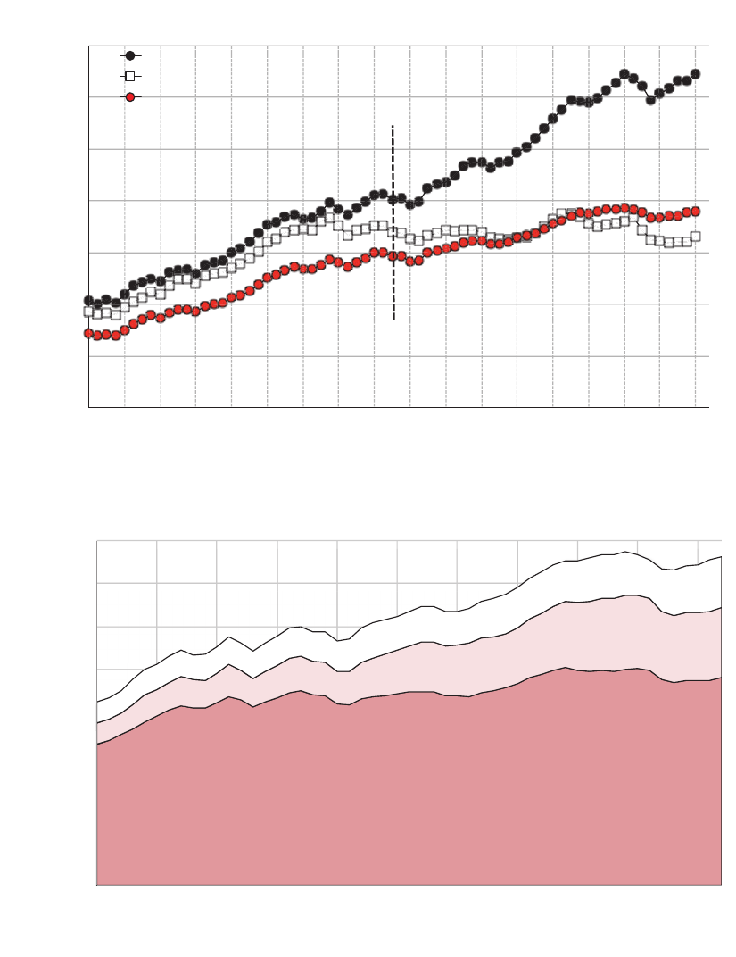
Figure 13: Growth for the bottom 90%

10,000

20,000

30,000

40,000

50,000

60,000

70,000

1946

1950

1954

1958

1962

1966

1970

1974

1978

1982

1986

1990

1994

1998

2002

2006

2010

2014

Average income in constant 2014 dollars

Bottom 90% income growth: Pre-tax income vs. fiscal income

National income per adult

Bottom 90% fiscal income per tax unit (Piketty-Saez)

Bottom 90% pre-tax income per adult

Source: Appendix Table II-B3 and Piketty and Saez (2003, updated to 2014)

+2.0%

+1.8%

+1.4%

+0.8%

+2.1%

-0.1%

5,000

10,000

15,000

20,000

25,000

30,000

35,000

40,000

1962

1967

1972

1977

1982

1987

1992

1997

2002

2007

2012

Average income in constant 2014$

Average pre-tax income of the bottom 90%

Taxable labor income

Capital income

Tax-exempt labor income

Source: Appendix Table II-B2e

Notes: The top panel compares (i) the average real pre-tax national income of bottom 90% adults (with income

equally split between spouses), (ii) the average ﬁscal income of bottom 90% tax un it s as e st i mat ed by Piketty

and Saez (2003, updated to 2014), and (iii) average national income per adult. Bottom 90% pre-tax income

per adult and national income per adult ar e deﬂated by the nat i on al income deﬂator, while bottom 90% ﬁscal

income per tax unit is deﬂated by the CPI used by Piketty and Saez. The numbers report the real annualized

income growth rate over 1946-1980 and 1980-2014. The bottom panel decomposes the pre-tax national income

of bottom 90% adults (wit h income eq u all y spl i t between spouses) into taxable labor income, tax-exempt labor

income (employee fringe beneﬁts and employer payroll taxes), and capital income.

Figure 14: Bottom 50% Incomes in the US vs. Fran c e

2,000

4,000

6,000

8,000

10,000

12,000

14,000

16,000

18,000

20,000

1962

1966

1970

1974

1978

1982

1986

1990

1994

1998

2002

2006

2010

2014

Average income in constant 2014 dollars

Average pre-tax income of bottom 50%

adults: United States

Average pre-tax income of bottom 50%

adults: France

Notes: The ﬁgure depicts the average pre-tax national income of the bottom 50% adults from 1962 to 2014 in

the United States and France. The unit is the individual adult and incomes within married couples are split

equally. Series for France are expressed in 2014 US dollars using a Purchasing Power Parity exchange rate of

.819 Euros per US dollar as estimated by the OECD. Estimates for France are from Garbinti, Goupille, and

Piketty (2016).