COPYRIGHT
FOUNTAINHEAD PRESS
Reaction Kinetics--Spectrophotometric
Determination of a Rate Law
Objective: Investigate the effect of reactant concentrations on the rate of reaction; to use
kinetics data to derive a rate law for the decomposition of crystal violet; to
calculate the rate constant for the reaction
Materials: Stock solutions of crystal violet (1.0 x 10
-4
M) and sodium hydroxide (0.10 M
NaOH)
Equipment: Two 10.0 mL graduated cylinders; one 50-mL beaker; two 100-mL beakers; one
250-mL beaker (waste); one 100-mL volumetric flask; three 10.00-mL pipettes;
spectrophotometer and cuvettes; stopwatch or timepiece with a second hand
Safety: Sodium hydroxide solutions are caustic; wash thoroughly if contact is made
with skin. Safety goggles should be worn at all times in the lab.
Waste
Disposal:
Excess reagents/reaction solutions may be flushed down the sink with water.
INTRODUCTION
Chemical kinetics is the study of reaction rate, or how fast a reaction proceeds. Knowing the
factors that control the rate of reactions has tremendous implications in both industry and the
environment. Manipulating these factors to increase the rate of a reaction can increase the yield
of desirable products of industrial processes, or decrease the rate of undesirable reactions to
minimize negative environmental impacts.
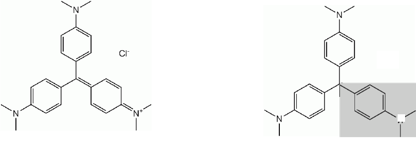
A reaction that readily lends itself to kinetic investigations is the reaction between crystal violet
and hydroxide ion. Crystal violet (CV), also known as Gentian violet or aniline violet, has many
applications, including use as a textile dye, as a histological stain for classifying bacteria, and as
a DNA stain in gel electrophoresis. In alkaline solutions, crystal violet reacts with hydroxide
according to reaction (1).
(1)
+ OH
-
(aq)
OH
N
(purple-blue)
(colorless)

COPYRIGHT
FOUNTAINHEAD PRESS
We can write a generic rate law relating the reaction rate to the concentration of reactants:
[ ]
[ ]
CV
Rate = C
V OH
time
z
x
k
−
∆
=
∆
(2)
The rate of the reaction is defined as the change in concentration of CV as a function of time,
and x and z represent the order of the reaction with respect to the reactants. The values of x and
z cannot be determined simply by examination of the balanced equation, but must be determined
experimentally. To simplify the experiment, the concentration of one reactant is typically held
constant while the other reactant concentration is varied. Any changes in the rate of the reaction
must be due to the change in the concentration of the varying reactant. By varying the
concentrations of reactants in Reaction (1), and observing the effect of the change in
concentration on the rate of the reaction, we can mathematically determine the values of x and z
in the rate law. Once the rate law is known, we can use the rate law and experimental data
(rates, concentrations) to calculate the value of the rate constant, k, at a given temperature.
We can modify the rate law in equation (2) by taking the log of both sides to yield:
[ ]
( )
( )
[ ]
x -z -
Δ CV
ln(rate) = = ln k[CV] [OH ] = ln k + xln CV + zln OH
Δtime
(3)
This equation takes the form of a straight line: y = mx + b. In one set of experiments, we hold
the concentration of crystal violet constant while varying the concentration of OH
-
. Plotting the
ln(rate) vs the ln[OH
-
], we obtain a straight line with a slope m = z and an intercept b = (ln(k) +
x ln[CV]). Similarly, we can hold the concentration of hydroxide constant while varying the
concentration of CV. A plot of ln(rate) vs the ln[CV] produces a straight line with a slope m = x
and an intercept b = (ln(k) + z ln[OH
-
]). Alternatively, we can take advantage of the integrated
forms of the rate law in which the rate law expression is integrated with respect to time:
1st Order: rate = k[A] ln [A]
t
= -kt + ln[A]
o
(4)
2nd Order: rate = k[A]
2
1/[A]
t
= kt + 1/[A]
o
(5)
Both equations (4) and (5) take the form of a straight line: y = mx + b. If the reaction is 1st
order in A, a plot of ln[A] vs. time should yield a straight line with a slope m = k. If the reaction
is 2nd order in A, a plot of 1/[A] vs. time should yield a straight line with a slope m = k.
But how can we measure the rate of this reaction? Crystal violet is a highly colored compound
and absorbs light in the visible region of the electromagnetic spectrum. Therefore, we can
monitor the rate of the reaction by monitoring the change in the concentration of CV over time
using spectrophotometric analysis.

COPYRIGHT
FOUNTAINHEAD PRESS
Spectrophotometric Analysis
Molecules will absorb light of a given wavelength if the energy of the light matches an electronic
transition within the molecule. The amount of light absorbed is defined by Beer’s Law, shown in
Equation 6:
= (6)
where A is the amount of light absorbed, and c is the concentration of the absorbing species. The
amount of light absorbed will also depend on the efficiency of the absorption process,
represented by the molar absorptivity coefficient (ε), and the path length of light traveling
through the solution (b).
A spectrophotometer is an instrument consisting of a light source, a sample cell, and a
photodetector. Light from the source is directed through the sample cell to the detector. A
spectrophotometer can display data using two different scales. Transmittance is defined as the
ratio of light reaching the detector when an absorbing species is in the sample cell compared to
the amount of light reaching the detector when a “blank” or non-absorbing solution is in the
sample cell. Transmittance is reported as %T,
% =
(
)
(
)
100 (7)
where (I)
a,
(I)
o
represent the intensity of light reaching the detector for the sample and blank
solutions, respectively. The other scale is absorbance, related to %T as shown in Equation 7.
A = 2.000 – log(%T) (8)
Absorbance is the preferred scale because it is linearly related to concentration, as shown in Eq.
8. The concentrations of unknown solutions can be determined using absorbance data and a
calibration plot known as a Beer’s Law plot, as shown in Figure 1. In this lab we will use
spectrophotometry to determine the rate law for the reaction shown in Reaction 1. Since the
absorbance of the reaction solution is directly related to the concentration of CV, the change in
absorbance over time is directly related to the change in CV concentration:
[ ]
[ ]
CV Abs
Rate =
time time
∆∆
=
∆∆
(9)

COPYRIGHT
FOUNTAINHEAD PRESS
Figure 1. A typical Beer’s Law plot.
0
0.1
0.2
0.3
0.4
0.5
0.6
0.7
0 10 20 30 40
Absorbance (A)
Concentration (M x 10
8
)
A = 0.46, Conc. = 2.3 x 10
-7
M
COPYRIGHT
FOUNTAINHEAD PRESS
Pre-Lab Questions
1. Why is the concentration of crystal violet held constant in these experiments, while the
concentration of sodium hydroxide is held varied?
2. Consider the following balanced chemical reaction:
2 MnO
4
-
(aq) + 5 H
2
O
2
(aq) + 6 H
+
(aq) 2 Mn
2+
(aq) + 5 O
2
(g) + 8 H
2
O(l)
a) A student wrote the following rate law for this reaction:
Rate = k [MnO
4
-
]
2
[H
2
O
2
]
5
[H
+
]
6
Is this correct? Explain.
b) Briefly describe what must be done to obtain the correct rate law.
3. Define the following terms:
a) Rate :
b) Rate law :
c) Rate constant, k :
COPYRIGHT
FOUNTAINHEAD PRESS
4. What would you expect to happen to the rate of the reaction between crystal violet and
hydroxide as temperature increases? Explain your answer in terms of kinetic theory. (refer
to the appropriate chapter/section of textbook).

COPYRIGHT
FOUNTAINHEAD PRESS
PROCEDURE
Part A. Beer’s Law Plot.
1. A typical spectrophotometer is illustrated in Figure 2. Note the knobs in the figure for
wavelength control, zero adjust, and 100% adjust. Using the wavelength control, adjust the
wavelength on your spectrophotometer to 590 nm. With no sample in the sample holder,
adjust the %T reading on the meter to zero using the zero adjust knob.
Figure 2. A typical spectrophotometer.
2. Obtain a cuvette and fill it with DI water. Carefully clean the surface of the cuvette as
illustrated in Figure 3. Insert the cuvette into the sample holder as shown in Figure 4 so the
reference line on the cuvette is aligned with the mark on the sample cell. Close the holder
cover and adjust the %T reading to 100% with the 100% adjust knob. Repeat steps 1 and 2
until you obtain stable 0% and 100% readings.
Figure 3. Handling/cleaning of a cuvette. Figure 4. Inserting cuvette into sample holder.

COPYRIGHT
FOUNTAINHEAD PRESS
3. Prepare a standard solution by pipetting 30.0 mL of the stock crystal violet solution to a
100.0-mL volumetric flask and adding DI water to the mark and mixing well. Pipette 10.0
mL of this standard solution and 10.0 mL of DI water into a 50-mL beaker. When the
solution is well mixed, fill a spectrophotometer cuvette with the solution. Clean the surface
of the cuvette and place it in the spectrophotometer as illustrated in Figures 3 and 4.
4. Calculate the concentration of the solution prepared in step 3 and record this concentration
as S1 in Table 1 on the Data Sheet. With the spectrophotometer wavelength set to λ
max
=
590 nm, record the absorbance of this solution. Discard the solution in the cuvette to the
waste container. Transfer 10.0 mL of the solution prepared in the 50-mL beaker in step 3 to
another clean 50-mL beaker, and add an additional 10.0 mL of water and mix well.
Calculate the concentration of this new solution and record it as S2 in Table 1 on your Data
Sheet. Rinse the cuvette with a few mL of this solution and discard the rinse in the waste
container. Fill the cuvette with the new solution, insert it into the spectrophotometer and
record the absorbance on your Data Sheet.
5. Repeat the dilution procedure in step 4 (serial dilution) until you have obtained absorbance
readings for 5 separate solutions. Be sure to calculate and record the concentrations of
solutions S3--S5 on you Data Sheet, and to record the absorbance of each solution.
Part B. Preparation of Reaction Solutions and Reaction Kinetics
I. Determination of Reaction Order for Hydroxide.
6. Fill one of the 100-mL beakers with about 50–60 mL of the stock solution of 0.10 M
NaOH. Obtain a 250-mL beaker and label it “Waste.”
7. Obtain two clean, dry 10-mL graduated cylinders, and label them “A” and “B.” Obtain a
clean, dry 50-mL beaker. Using a pipette, transfer 10.0 mL of the crystal violet solution
prepared in part A from the 100.0-mL volumetric flask to graduated cylinder A. Using a
different pipette, transfer 10.0 mL of the stock NaOH solution obtained in step 6 to
graduated cylinder B. These solutions will be used to prepare reaction mixture E1, as
indicated in Table 1.
Table 1. Solution Volumes for Reaction Mixture E1--E5
Reaction Mixture
Volume of Crystal
Violet (3.0 x 10
-5
M)
Volume of DI Water
Volume of NaOH
(0.10 M)
E1
10.0 mL
0.0 mL
10.0 mL
E2
10.0 mL
2.0 mL
8.0 mL
E3
10.0 mL
4.0 mL
6.0 mL
E4
10.0 mL
6.0 mL
4.0 mL
E5
10.0 mL
8.0 mL
2.0 mL
COPYRIGHT
FOUNTAINHEAD PRESS
8. Transfer the 10.0 mL of crystal violet solution to the 50-mL beaker. While Student 1 adds
the contents of graduated cylinder B to the beaker and mixes well, Student 2 should start
the stopwatch. After mixing well, Student 1 will transfer some of solution E1 to a clean,
dry cuvette and insert the cuvette into the spectrophotometer, following the procedures
illustrated in Figures 3 and 4.
9. At t = 10 seconds, Student 1 will read the % transmittance of the solution, and Student 3
will record this reading on the Data Sheet in Data Table 2 in the column labeled E1. While
Student 2 continues to mark the time in 10 second intervals, Student 1 should read out the
% transmittance measurement at each time and Student 3 should record the corresponding
reading in Data Table 2 in the column for E1. Continue recording % transmittance
measurements as a function of time for a total of 250 seconds.
10. Discard the cuvette sample and reaction solution from the 50-mL beaker in the waste
beaker.
11. Clean and dry both 10.0-mL graduated cylinders, the 50-mL beaker, and the cuvette.
12. Repeat steps 7–11 using the solution volumes indicated in the table for reaction mixture E2.
The NaOH and DI water will both be placed in graduated cylinder B.
13. Repeat until % transmittance vs time data have been obtained for all solutions E2--E5.
CALCULATIONS
Part A. Beer’s Law
1. Plot the absorbance measurement obtained for each of the standard solutions in Data Table1
vs. the calculated [CV]. You may use either the graph paper provided or you may plot the
data using a spreadsheet (e.g., Excel). If you use a spreadsheet program, be sure to select
the “scatter plot” option when plotting the data. Based on Beer’s Law, this plot should
produce a straight line. Calculate the slope of this line, and record your result on the Data
Sheet as ε. The accepted literature value of λ
max
= 87,000 M
-1
cm
-1
. Compare your calculated
value with the accepted value, and calculate the percent error as:
Percent error = [(accepted value – experimental value)/(accepted value)] x 100
Record your % error on the Data Sheet.
Part B. Rate Law
In order to determine the rate law we will need to determine the rate (in units of M/sec), the
order of the reaction with respect to the reactants (m and n), and the value of the rate constant, k.
To determine the rate, we will need to know the original concentration of the reactants and how
long it took them to react.
COPYRIGHT
FOUNTAINHEAD PRESS
1. Reaction Rates. For each of the reactions E1 through E5, calculate the absorbance the
absorbance from % transmittance using Eq. 8 and plot the absorbance of the solution vs.
time. You may either plot the data on the graph paper provided, or you can enter the data
into a spreadsheet (e.g., Excel).
The rate of a given reaction is calculated as the initial slope of the plot of absorbance vs
time. If you view the plot, the slope may decrease over time, so it is important to calculate
the slope in the initial portion of the graph (i.e., first 100 to 200 seconds) in a region where
the plot appears to be linear. If you are using a spreadsheet program, you can take advantage
of the “add trend line” option to calculate the best-fit straight line, which will include a
calculation of the slope.
Record the reaction rates for each reaction mixture on the Calculation Sheet.
2. Reaction order. Since the CV concentration was monitored spectrophotometrically, the
absorbance of the reaction solution was directly related to the [CV] by Beer’s Law.
Therefore, we can take advantage of the integrated rate laws to determine the order of the
reaction with respect to CV. Using the absorbance data vs. time for reaction E1, calculate
ln[Abs] and 1/[Abs] for each data point and record these data in Data Table 3.
Using experimental data for reaction mixture E1, prepare two graphs. For the first order
graph, plot ln[Abs] vs. time; for the second order graph, plot 1/[Abs] vs. time. You can plot
the data using the graph paper provided or you can use a spreadsheet program (e.g., Excel).
Based on the graph that produces a straight line, record the value of x on the Data Sheet.
To determine the value of z we take advantage of the fact that only one reactant
concentration was changed during the experiment. Note that the [CV] was the same for
Reactions E1--E5, while the [OH
-
] varied. The generic rate law can be written as
Rate = k [CV]
x
[OH
-
]
z
Taking the natural log of both sides of the equation yields:
ln rate = lnk + xln[CV] + z ln[OH
-
] (3)
Since x and [CV] are both constants for E1--E5, we can combine them with ln k to make a
new constant ln k’, which yields:
ln rate = lnk’ + z ln[OH
-
] (10)
This new equation resembles the equation for a straight line, y = mx + b. Plotting ln rate vs.
ln [OH
-
] for experiments E1--E5 yields a straight line with a slope = z.
Using the volumes and concentrations for CV and NaOH solutions, calculate the initial
concentration of CV and OH
-
in each of the reactions E1--E5, and record these
concentrations under Part B3 in Calculations. Using the rates for E1--E5, plot ln rate vs. ln
[OH
-
]. Calculate the slope of this plot and record it as z on your Calculations Sheet. You
should round your results to the nearest integer.

COPYRIGHT
FOUNTAINHEAD PRESS
3. Rate Constant. We now know the exact form of the rate law from Part B1 and B2. We can
rearrange the rate law expression to solve for the rate constant, k.
x-
Rate
k =
[CV] OH
z
(11)
Using Eq. (11), calculate the value of k for each of the reaction mixture E1--E5. For the
calculation of reaction orders, we calculated reaction rate as a change in absorbance vs.
time. In order to obtain appropriate units for k, we must first calculate the rate in appropriate
units, or as a change in concentration of CV vs time. On the Calculations Sheet, record the
initial concentration of CV for each reaction mixture E1--E5. Using the measured
absorbance at t = 100 seconds and the Beer’s Law plot from Part A, determine the [CV] at t
= 100 sec. Record this concentration for each reaction mixture E1--E5 in Part 3 on the
Calculations Sheet. The rate of the reaction for each mixture can now be calculated as
Rate (M/s) = ([CV]
o
– [CV]
t=100
) /100 sec. (12)
Record these calculate rates in Part 3 on the Calculations sheet. The value of k for each
reaction mixture can now be calculated using Equation (11). Record the calculated values
of k for reactions E1--E5, and use these values to calculate and record an average value of k.

COPYRIGHT
FOUNTAINHEAD PRESS
Data Sheet: Reaction Kinetics
Part A. Beer’s Law Plot
λ
max
= _______________ nm
Data Table 1.
Standard Solution [Crystal Violet] (M) Absorbance
S1. ________________ __________
S2. ________________ __________
S3. ________________ __________
S4. ________________ __________
S5. ________________ __________
Calculated ε: _______________
Percent error in ε: _____________
Calculations:
COPYRIGHT
FOUNTAINHEAD PRESS
Data Sheet: Reaction Kinetics (cont.)
Part B. Reaction Solutions and Reaction Kinetics
Data Table 2. % Transmittance Readings vs. Time for Reaction Solutions E1--E5
Time
E1
E2
E3
E4
E5
10 __________ __________ __________ __________ __________
20 __________ __________ __________ __________ __________
30 __________ __________ __________ __________ __________
40 __________ __________ __________ __________ __________
50 __________ __________ __________ __________ __________
60 __________ __________ __________ __________ __________
70 __________ __________ __________ __________ __________
80 __________ __________ __________ __________ __________
90 __________ __________ __________ __________ __________
100 __________ __________ __________ __________ __________
110 __________ __________ __________ __________ __________
120 __________ __________ __________ __________ __________
130 __________ __________ __________ __________ __________
140 __________ __________ __________ __________ __________
150 __________ __________ __________ __________ __________
160 __________ __________ __________ __________ __________
170 __________ __________ __________ __________ __________
180 __________ __________ __________ __________ __________
190 __________ __________ __________ __________ __________
200 __________ __________ __________ __________ __________
210 __________ __________ __________ __________ __________
220 __________ __________ __________ __________ __________
230 __________ __________ __________ __________ __________
240 __________ __________ __________ __________ __________
250 __________ __________ __________ __________ __________

COPYRIGHT
FOUNTAINHEAD PRESS
Calculations
Data Table 3. Absorbance Readings vs. Time for Reaction Solution E1
Time ____Absorbance ln (Abs) 1/(Abs)
10 ____________ ____________ ____________
20 ____________ ____________ ____________
30 ____________ ____________ ____________
40 ____________ ____________ ____________
50 ____________ ____________ ____________
60 ____________ ____________ ____________
70 ____________ ____________ ____________
80 ____________ ____________ ____________
90 ____________ ____________ ____________
100 ____________ ____________ ____________
110 ____________ ____________ ____________
120 ____________ ____________ ____________
130 ____________ ____________ ____________
140 ____________ ____________ ____________
150 ____________ ____________ ____________
160 ____________ ____________ ____________
170 ____________ ____________ ____________
180 ____________ ____________ ____________
190 ____________ ____________ ____________
200 ____________ ____________ ____________
210 ____________ ____________ ____________
220 ____________ ____________ ____________
230 ____________ ____________ ____________
240 ____________ ____________ ____________
250 ____________ ____________ ____________
COPYRIGHT
FOUNTAINHEAD PRESS
Calculations (con’t.)
Part B. Reaction Rates
1. Reaction Mixture Reaction Rate ( ∆[Abs] / ∆time) [CV]
o
[OH
-
]
o
E1 ________________________ ___________ ___________
E2 ________________________ ___________ ___________
E3 ________________________ ___________ ___________
E4 ________________________ ___________ ___________
E5 ________________________ ___________ ___________
2. Reaction Orders: [CV], x = ______________ [OH
-
], z = ______________
3. Reaction Mixture [CV]
o
[CV]
t=100
Rate [OH
-
]
o
k
E1 __________ __________ __________ __________ __________
E2 __________ __________ __________ __________ __________
E3 __________ __________ __________ __________ __________
E4 __________ __________ __________ __________ __________
E5 __________ __________ __________ __________ __________
Average k (with units!) = ______________

COPYRIGHT
FOUNTAINHEAD PRESS

COPYRIGHT
FOUNTAINHEAD PRESS

COPYRIGHT
FOUNTAINHEAD PRESS

COPYRIGHT
FOUNTAINHEAD PRESS
COPYRIGHT
FOUNTAINHEAD PRESS
Post-Lab Questions
1. Based on your results, what is the order of the reaction with respect to CV? What is the order
of the reaction with respect to hydroxide ion? What is the overall order of the reaction?
2. A student inadvertently added hydroxide solution instead of DI water to the CV solution in
graduated cylinder A in Part B(II) of the Procedure. How would this affect the data collected
by the student, and how would it affect the reaction rate calculated from the plot of
absorbance vs. time?
3. Students in lab section #1 performed this experiment when the room temperature was 20 °C,
while students in lab section #2 performed this experiment when the room temperature was
28 °C. How would the reaction rates compare for lab sections #1 and #2? How would the
values of k compare?
4. Using procedures similar to this lab exercise, a student used the reaction rates based on
Absorbance measurements from Part B1 of the Calculations, rather than the rates calculated
from concentrations in Part B3. How would this affect the calculated value of k, and what
would be the units associated with this value?
