Can't Be Late: Optimizing Spot Instance Savings under Deadlines

This paper is included in the

Proceedings of the 21st USENIX Symposium on

Networked Systems Design and Implementation.

April 16–18, 2024 • Santa Clara, CA, USA

978-1-939133-39-7

Open access to the Proceedings of the

21st USENIX Symposium on Networked

Systems Design and Implementation

is sponsored by

Can’t Be Late: Optimizing Spot Instance Savings

under Deadlines

Zhanghao Wu, Wei-Lin Chiang, Ziming Mao, and Zongheng Yang, University of

California, Berkeley; Eric Friedman and Scott Shenker, University of California, Berkeley,

and ICSI; Ion Stoica, University of California, Berkeley

https://www.usenix.org/conference/nsdi24/presentation/ wu-zhanghao

Can’t Be Late: Optimizing Spot Instance Savings under Deadlines

Zhanghao Wu, Wei-Lin Chiang, Ziming Mao,

Zongheng Yang, Eric Friedman

†

, Scott Shenker

†

, Ion Stoica

University of California, Berkeley

†

UC Berkeley and ICSI

Abstract

Cloud providers offer spot instances alongside on-demand

instances to optimize resource utilization. While economically

appealing, spot instances’ preemptible nature causes them

ill-suited for deadline-sensitive jobs. To allow jobs to meet

deadlines while leveraging spot instances, we propose a

simple idea: use on-demand instances judiciously as a backup

resource. However, due to the unpredictable spot instance

availability, determining when to switch between spot and

on-demand to minimize cost requires careful policy design. In

this paper, we ﬁrst provide an in-depth characterization of spot

instances (e.g., availability, pricing, duration), and develop a

basic theoretical model to examine the worst and average-case

behaviors of baseline policies (e.g., greedy). The model serves

as a foundation to motivate our design of a simple and effective

policy, Uniform Progress, which is parameter-free and requires

no assumptions on spot availability. Our empirical study, based

on three-month-long real spot availability traces on AWS,

demonstrates that it can (1) outperform the greedy policy by

closing the gap to the optimal policy by 2

in both average

and bad cases, and (2) further reduce the gap when limited

future knowledge is given. These results hold in a variety of

conditions ranging from loose to tight deadlines, low to high

spot availability, and on single or multiple instances. By im-

plementing this policy on top of SkyPilot, an intercloud broker

system, we achieve 27%-84% cost savings across a variety of

representative real-world workloads and deadlines. The spot

availability traces are open-sourced for future research.

1 Introduction

As organizations continue to migrate their workloads to

clouds, the need to minimize operational costs has become

a critical concern [41]. One of the top contributors to cloud

spending is the cost of compute instances [8], which are

typically offered in two pricing models: on-demand and spot.

On-demand instances are available but come at a premium

See spot traces:

https://github.com/skypilot-org/spot- traces

In this paper, we do not consider “reserved” instances, whose economics

involves volume contracts and is more complex.

V100 GPU 64-core CPU

AWS 3× 2–6×

Azure 3–6× 3–10×

GCP 3× 4–11×

Table 1: Cost savings of spot vs. on-demand instances.

cost. In contrast, spot instances are typically 3–10

cheaper

(Table 1), but are less available and they can be preempted unex-

pectedly. As a result, more applications such as analytics [13],

AI [28, 37, 40], HPC [29], and CI/CD workloads [1], are lever-

aging spot instances to reduce costs. To handle preemptions,

these jobs either checkpoint periodically and recover from the

last checkpoint on restart [25,46], or re-execute the entire job.

However, while many applications can tolerate uncertainties

introduced by spot instance preemptions, others cannot. One

such category is delay-sensitive applications where a job needs

to ﬁnish by a certain deadline [24]. Examples include process-

ing new user data to keep an AI model up-to-date in a recom-

mendation system, or analyzing the latest information to make

timely decisions in a trading application. Therefore, most of

deadline-sensitive applications eschew spot instances in favor

of on-demand instances, thus trading off cost for predictability.

In this paper, we resolve this tradeoff by enabling an applica-

tion to leverage spot instances while still meeting its deadline.

For simplicity, we focus on recoverable jobs running on a sin-

gle instance, and assume the running time of the job is known,

as well as its deadline. A job can be in one of three states:

(1) running on a spot instance, (2) running on an on-demand

instance, or (3) idle, i.e., waiting for a spot instance to become

available. We design scheduling policies that periodically

decide whether a job should remain in the same state or switch

to another state. When a job switches to a non-idle state we as-

sume there is a delay, e.g., the overhead of provisioning/setting

up a new instance, and re-starting from a previous checkpoint.

Due to the high unpredictability in spot instance availability

(§2.2), the key challenge lies in striking a balance between cost

optimization and deadline adherence to effectively leverage

the low cost of spot instances without missing the deadline.

A simple solution to this problem would be for a job to

USENIX Association 21st USENIX Symposium on Networked Systems Design and Implementation 185

use a spot instance up to the point at which the remaining

computation time equals the remaining time to deadline, and

then switch to an on-demand instance until it ﬁnishes. While

this “greedy” policy (§3.4) guarantees that the job will meet

its deadline, we show that it is sub-optimal. We do so by

developing a theoretical framework to study the worst-case

behavior (e.g., competitive ratio) of the policy (§4).

To address the limitations of “greedy” policy, we propose

a simple and effective policy, called Uniform Progress, which

aims to make uniform progress towards deadline, by distribut-

ing the job computation uniformly across the time. Uniform

Progress requires no assumption about spot instances’ avail-

ability and is parameter-free. Using simulations on real-world

traces we show that Uniform Progress outperforms greedy pol-

icy and approaches an optimal policy with limited knowledge

of the future (knowing how long the next spot instance is going

to last) in a variety of scenarios—from loose to tight deadlines,

and from low to high spot availability. We build a prototype

of Uniform Progress and evaluate it in a cloud setting on three

real-world workloads: ML training, scientiﬁc batch jobs, and

data analytics. Results show that Uniform Progress achieves

27–84% cost savings while meeting deadlines.

This paper is organized as follows. First, we provide an

in-depth characterization of spot instances across various

cloud regions, examining their availability patterns, pricing,

and lifetime to inform our policy design (§2). Next, we develop

a theoretical model that captures the essential dynamics of

spot instances, which enables us to examine the worst-case

behavior of a given policy (§3, §4). We then present our

policies for jobs with both single and multiple instances (§5)

and conduct a comprehensive empirical study on months-long

real-world traces of spot instances (§6). We build a prototype

implementation that supports the proposed policies in a

cloud setting, and evaluate these policies on three real-world

workloads (§7). Finally, we review related work in §8.

In summary, this paper makes the following contributions:

We introduce a problem of using spot instances to min-

imize the cost of running a job with deadline adherence.

We develop a theoretical framework to study the worst

and average-case behavior of baseline policies, providing

insights on the tradeoff between cost and deadline.

We propose Uniform Progress, a simple but effective pol-

icy which is parameter-free and requires no assumptions

on spot availability. Empirically, we show the signiﬁcant

improvement of the policy in a wide variety of scenarios.

We implement a prototype system with Uniform Progress,

and evaluate it on real-world workloads.

Finally, we open source our three-month traces of spot instance

availability to encourage future research in this area.

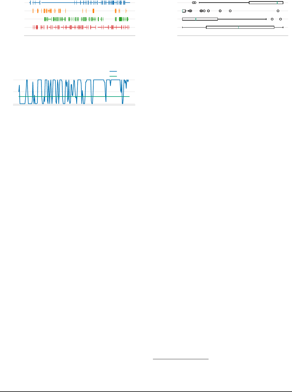
2 Characterization of Spot Instances

In this section, we characterize spot instance availability and

pricing over time and across availability zones. We observe

high volatility in availability but a smooth pricing pattern. We

04/22 04/24 04/25 04/27 04/28 04/30

Availability

Preemption

Figure 1: Real spot preemptions and availability are highly

correlated. Trace is in AWS us-west-2b. Upper: preemptions.

Horizontal lines represent a running spot instance. Vertical

bars are preemptions. Lower: availability. Horizontal lines are

spot instance available periods. Vertical bars are changes from

availability to unavailability. Grey gaps are unavailability pe-

riods. Note that although some vertical bars look immediately

followed by a horizontal line, there are still gaps in between.

use these insights to drive the design of our scheduling policy.

2.1 Methodology of Spot Trace Collection

We collect spot availability traces from public clouds. A

trace is a time series showing whether a particular spot instance

type is available at a given time in a zone. We collect these

traces over a three-month period and in nine AWS availability

zones (three in us-west-2, four in us-east-1, two in us-east-2).

A key challenge of trace collection is that it can be pro-

hibitively expensive. For example, a spot V100 instance costs

about $1/hour. If we collect a real preemption trace where an in-

stance is kept live as much as possible modulo preemptions, col-

lecting three-month long traces in all nine zones could cost over

$10,000. Instead, we propose an approximation: we collect

availability traces, where we try to launch a spot instance every

10 minutes to probe if it is available and then immediately termi-

nate it. To validate this approach, Figure 1 shows a high correla-

tion between the real preemption and availability signals over

a week-long period. This approach reduces the cost of trace

collection by about

100×

. For completeness, we also include

real preemption traces in our evaluation of policy performance

on multi-instance jobs (§6.6) and real-world workloads (§7.2).

In this work, we focus on a few scarce instance types, i.e.,

Nvidia V100 and K80 GPU instances, which are now in high

demand [4] due to the rise of Generative AI and large language

models (LLMs). Focusing on these scarce instance types is thus

both useful and interesting, as they are frequently preempted,

providing a good testing ground for scheduling policies.

2.2 High Variance in Spot Availability

Our analysis reveals that spot availability varies signiﬁcantly

across zones and over time. Figure 2 (left) shows the avail-

ability traces of 9 AWS zones over 2 weeks (4 example zones

are in Figure 2 and the rest 5 zones are in §A.1). We observe

a large difference across zones (e.g., us-west-2a vs us-east-1a).

The periods of unavailability can last for hours or even days.

To understand spot availability distributions, we overlay

6-hour windows on a 2-week period (thus,

14 × 24/6 = 56

windows per zone) and count the fraction of availability

probes that succeeded in each window. Figure 2 (right)

plots the distributions of spot availability fractions in the 56

windows per zone, which approximate the fraction of time

spot instances are available in each zone. We observe that each

186 21st USENIX Symposium on Networked Systems Design and Implementation USENIX Association

02/17 02/19 02/22 02/24 02/27 03/01

us-east-2b

us-east-1d

us-east-1a

us-west-2a

0% 20% 40% 60% 80% 100%

us-east-2b

us-east-1d

us-east-1a

us-west-2a

Figure 2: Spot Availability is highly unpredictable and volatile. Traces are across four of nine AWS zones collected. Left: Availability.

Horizontal lines are available periods. Vertical bars are changes from available to unavailable, followed by grey gaps indicating un-

available period. Right: Boxplots of spot availability fraction, i.e., percentage of the time an instance is available in 6-hour windows.

02/17 02/20 02/23 02/26 03/01

50%

100%

us-east-2a

Availability

Price ratio

Figure 3: High volatility of spot availability fraction. Avail-

ability can jump from 100% to 0% within hours. Price ratio:

spot price divided by on-demand price.

zone can go from being highly available to mostly unavailable

across time (e.g., in us-east-2b, the difference between p25

and p75 is about 70%) and there is little correlation across

zones. In addition, Figure 3 shows changes in spot availability

fractions over time. We observe a highly volatile pattern:

availability can change from 100% to 0% within hours.

The results above suggest that scheduling policies should

be robust to highly unpredictable availability patterns. For

generality, in this paper, we make no assumptions on spot

availability patterns. We discuss existing prediction-based

approaches in §8 and leave this direction to future work.

2.3 Relative Stability in Spot Pricing

In contrast, we observe that spot pricing is much more stable

than availability. Figure 3 shows the price ratio of spot to

on-demand for AWS stays almost constant despite signiﬁcant

changes in availability. In the three-month-long trace, we ob-

serve only a 5% price variation on average over any one-week

period, validating the recently introduced smooth pricing

model on AWS [5]. GCP’s spot instance prices are even more

stable as it is guaranteed to only change once every 30 days [3].

2.4 Correlation of Multi-Instance Availability

To understand the behavior of multiple spot instances, we

analyze 2-week preemption traces and 2-week availability

traces for clusters of 4 and 16 instances, respectively (see §6.1

for details). Notably, over 94% of the time, either all or none of

the instances are available in each cluster. This suggests avail-

ability tends to change simultaneously for multiple instances

(bulk preemption is also observed in [16]), up to a count of 16.

3 Using Spot for Deadline-Sensitive Jobs

In this section, we present a simple model to formulate the

problem, discuss when a policy matters, and then give three

rules for policy design followed by a basic greedy policy.

3.1 Problem Setup

We consider two types of instances with the same hardware:

an on-demand instance, which is always available,

and a spot

instance, whose availability is unpredictable. We assume that

spot availability is non-adversarial, meaning that it is indepen-

dent of the job’s choices and observable factors, except for §4.1,

where we adopt competitive analysis for the worst case study.

We focus on long-running (hours to days) jobs where

preemptions are likely. We ﬁrstly assume each job uses one

instance. We will extend it to multiple instances in §5.5 and

evaluate it in §6.6.

For a deadline-sensitive job, we denote remaining compu-

tation time at time

C(t)

and remaining time-to-deadline as

R(t)

. This implies that the job’s total computation time is

C(0)

and deadline is

R(0)

. Based on the deﬁnition, we can derive that

R(t) =R(0)−t and when a job is progressing, ∂C(t)/∂t =−1.

We assume that both

C(0)

and

R(0)

are given and the

job is fault-tolerant to interruptions. For example, ML

training typically has a consistent per-epoch time, indicating

a predictable total runtime, and the model weights can be

checkpointed and resumed for fault tolerance. Additionally,

computation times for many recurring jobs (e.g., data analytics,

scientiﬁc HPC, CI/CD) can be derived from past executions.

To account for overheads of starting the job on a new

instance, we introduce changeover delay,

, which includes the

time required to launch an instance, set up dependencies, and

recover any potential progress loss caused by gaps between

checkpoints or restarting the most recent unsaved execution.

Whenever a job switches to a new spot or on-demand instance,

a changeover delay occurs, meaning that

C(t)

does not

decrease for a duration of

while

R(t)

continues to decrement.

A delay

is charged at the new instance type’s price. Switching

from an instance to idle (i.e., termination) does not incur a

delay. We will extend the model to consider variety with

C(0)

and d in §5.6, and evaluate it in §6.7.

The goal is to minimize the cost for completing job’s

computation time

C(0)

before deadline

R(0)

, i.e.,

C(R(0)) ≤0

using spot and on-demand instances. For simplicity, we deﬁne

the price for an on-demand instance to be

k > 1

, and a spot

instance to be 1. We assume that cloud providers charge every

second when an instance is alive.

Based on the observation

This is a simplifying assumption. In practice, some on-demand instance

types can hit unavailability.

Cloud providers have different billing practices, e.g., AWS does not

USENIX Association 21st USENIX Symposium on Networked Systems Design and Implementation 187

IDLE

SPOT

Spot Availability

0 10 20 30 40 50 60

Elapsed Time (hours)

IDLE

SPOT

C(t) = R(t)

Optimal for d = 0 ($381.85)

(a) Without changeover delay.

0 10 20 30 40 50 60

Elapsed Time (hours)

IDLE

SPOT

C(t) = R(t) + 2d

Greedy for d > 0 ($658.13)

(b) With changeover delay.

Figure 4: Example decision traces of policies on real spot

availability on AWS.

in §2.3, we assume both the on-demand and spot price are

ﬁxed throughout the time before deadline R(0).

3.2 Scheduling Policy

At any time

, a job can be in one of the following three

states: idle, running on a spot instance, or running on an

on-demand instance. While we assume that on-demand

instances are always available, spot instances can be in one

of two states: available or unavailable. The job’s state space is

the combination of any of the instance state and the spot state,

except for an impossible case where the instance state is spot

with spot state unavailable (Table 2). A scheduling policy is

invoked to decide how a job moves across instance states.

Spot State \ Instance State Idle Spot On-Demand

Spot Available ① ③ ④

Spot Unavailable ② - ⑤

Table 2: State space for a job.

In the ideal case where changeover delay

d =0

, the problem

is simple. An optimal policy is to use a spot instance whenever

it is available, i.e., transition between state

②

and

③

, until

C(t) = R(t)

. After that, the job cannot stay idle, as it needs to

utilize all the remaining time before deadline to make progress.

Since there is no changeover delay, the policy can use spot

whenever it is available and switch to on-demand when it is

not, i.e., transition between

③

and

⑤

. This policy is optimal

because it utilizes all available spot instance lifetimes before

the deadline, without additional cost. Figure 4a shows an ex-

ample decision trace of how this policy performs for a job with

C(0) = 48

hours and

R(0)=60

hours on a real spot availability

trace, where the policy utilizes every spot lifetime, and runs

the remaining computation with on-demand instances.

However, when changeover delay

d >0

, which is the practi-

cal case, the problem becomes non-trivial. The policy now has

to decide whether it is worth switching to a different instance at

the expense of losing time

without making progress, which

increases the risk of missing the deadline. For example, apply-

ing the optimal policy above for

d >0

would result in missing

charge for spot instances preempted within the ﬁrst hour, while GCP does.

the deadline, since every switch costs an additional time d.

In the remainder of this paper, we focus on designing

policies for the more practical d > 0 scenario.

3.3 Rules for Policy Design

Based on the problem setting, we propose three basic rules

that all policies without future knowledge should follow to

avoid unnecessary cost or missing the deadline.

Thrifty Rule. The job should remain idle after C(t) = 0.

Safety Net Rule. When a job is idle and

R(t) < C(t) + 2d

switch to on-demand and stay on it until the end.

The policy is required to guarantee the job ﬁnished by

the deadline. After

R(t) < C(t) + 2d

becomes true, it is no

longer safe to move from idle to spot. Otherwise, when the

changeover delay of the spot ﬁnishes, the remaining time will

become

R(t) <C(t)+d

, which means any preemption to the

spot instance will result in missing deadline. Note that one

could wait until

R(t) =C(t)+d

then move to on-demand, but

there is no gain for waiting an additional d if the job is idle.

Exploitation Rule. Once start using a spot instance, stay on

it until it is preempted.

If the job is on a spot instance, any progress made will

always cost the minimum price any policy could get, i.e.,

the spot price. Voluntarily switching from spot to idle or

on-demand will have no beneﬁt, but less progress or more cost.

This rule will not violate the deadline because the Safety

Net Rule guarantees that

R(t) ≥ C(t) + 2d

holds at the

time

when the job is moved to the current spot instance.

After the changeover delay is incurred and the job starts

progressing,

R(t)−C(t)

will not change, i.e.,

R(t) ≥C(t)+d

holds, meaning the remaining time is enough for at least one

changeover even if the current spot is preempted. The job will

be able to switch to on-demand when Safety Net Rule kicks in.

3.4 Greedy Policy

Based on the three rules, we propose a straightforward

greedy policy. The greedy policy behaves as follows:

Stay on any available spot instance until it is preempted

(Exploitation Rule), and keep waiting if no spot instance

is available, i.e., transition between ② and ③ in Table 2.

(Safety Net Rule) When

R(t) <C(t)+2d

holds and the

job is idle, move to on-demand and stay there until the end.

In Figure 4b, we show the decision trace of the greedy policy

on the same spot availability trace as before (Figure 4a). The

greedy policy acts much more conservatively than the previous

optimal policy without changeover delay. That is because

greedy can no longer afford frequent switches between

on-demand and spot instances as before without missing the

deadline. Thus, we now turn our attention to: can we do better

than greedy while not assuming future knowledge?

4 Theoretical Analysis

In this section, we delve into theoretical aspects of the

problem and prove the existence of a policy that is better than

greedy in both worst and average cases.

188 21st USENIX Symposium on Networked Systems Design and Implementation USENIX Association

n-sliced greedy

6420

Shifted (n-1)-sliced greedy

Look for Spot Go to On-Demand

Figure 5: Example slicing for randomized shifted greedy (RSF)

policy, where deadline

R(0) = 6

, computation time

C(0) = 3

and slices n = 3. Dashed lines indicate boundaries of slices.

4.1 Worst Case with Competitive Analysis

We ﬁrst look into the worst case by investigating the

competitive ratio

of a policy without knowledge of future

spot availability, which is the ratio of the cost of the policy to

the best omniscient policy with full knowledge of future spot

availability. By “worst” case, we assume that spot instances

are chosen by an oblivious adversary, who can base their

decisions on complete knowledge of the job’s policy but not

on random coin ﬂips used by the policy. Our goal is to prove

that there is a policy with lower competitive ratio

than greedy,

i.e., performs better in the worst case.

To simplify the presentation, we assume changeover delay

is small and ignore the term

O(d)

. Also, we use

R(t) =C(t)+d

as Safety Net Rule’s condition, instead of

R(t) = C(t) + 2d

which will not affect the conclusion, due to negligible O(d).

A natural bound for

1 ≤ c ≤ k

, where

can be reached

when the oblivious adversary choose a case that a given policy

have to use all on-demand, and the omniscient policy could use

all spot instances. We can prove that for any

R(0)

C(0)

, a deter-

ministic policy cannot perform better than greedy (see §A.2.1).

Theorem 1. For any deterministic policy P, c ≥k−O(d).

With Theorem 1, we can conclude that a policy has to be ran-

domized to beat greedy, whose competitive ratio

c=k

, as an ad-

versary can simply make spot available from

′

, where

R(t

′

C(t

′

)+d

. We now construct a better policy on top of greedy.

We ﬁrst extend greedy to an

-sliced greedy policy, in which

we divide the time into

even slices with length

R(0)

and apply

greedy in each of these slices with

C(0)

progress to make. The

upper ﬁgure in Figure 5 is an example of

-sliced greedy, with a

deadline

R(0)=6

and 3 slices. In each slice, the policy enforces

the job to make ≥

C(0)

=1 units of progress within

R(0)

=2.

We then shift the

-sliced greedy policy by

C(0)

to get shifted

(n−1)

-sliced greedy policy, which uses on-demand for time

C(0)

from start (1 in the example Figure 5) and then applies

(n−1)-sliced greedy from t =

C(0)

until t =R(0)−

R(0)−C(0)

Although both policies have

c = k

, we can deﬁne a

randomized shifted greedy (RSF) policy by using either

the

-sliced or the shifted

(n − 1)

-sliced greedy with equal

probability at any time

. We can prove that the competitive

ratio for RSF is bounded and lower than greedy (see §A.2.1).

Theorem 2. If

R(0) ≥ 2C(0)

, then for RSF policy has

c≤

k+1

k−1

+O(d)<k.

When deadline

R(0)

is more than

2×

longer than computa-

50 100 150

Actual Greedy Cost

100

150

Theoretical Cost

pearsonr=0.97

(a) Theoretical vs actual greedy

cost with delay d =0.01h.

0 50

#Slices

0.1

0.2

Variance

us-east-1a

us-east-1f

us-east-2b

us-west-2c

(b) Variance vs number of slices

with an 80-hour deadline.

Figure 6: Numerical results for validating the theoretical

greedy cost and the assumption for increasing variance in the

stochastic model. Both analysis are conducted on sampling

sub-traces from 2-month AWS spot availability traces.

tion time

C(0)

, the worst case (the largest gap to omniscient pol-

icy) for RSF policy is bounded, i.e., provably better than greedy.

For

R(0) ≤ 2C(0)

, we can simply use on-demand until

R(t) = 2C(t)

then start using RSF policy. We denote this

modiﬁed RSF (MRSF) policy.

Corollary 1. Let

R(0)

C(0)

−1

for

0<a ≤1

. MRSF policy has:

c≤ k−ak+a(

k+1

k−1

)+O(d) =k−

a(k−1)(n−1)

+O(d) <k

With MRSF policy, we shown that there exists a policy that

performs better than greedy for any

R(0)

C(0)

in worst cases

by randomization and distributing job progress.

4.2 Average Case with Stochastic Model

Since spot availability is a complex stochastic process, we

propose a simpler model that is analytically tractable for the de-

velopment of practical policies. With that model, we will show

that n-sliced greedy is better than greedy in the average case.

In order to model the spot process, we consider a smoothed

version where we assume that a fractional spot is always

available, with a ratio

r <1

, i.e., a job running on the fractional

spot makes

amount of progress per unit of time. For example,

if spots have 4-hour average lifetimes and 1-hour average wait

times after preemption. Then, the fractional spot has a ratio,

r = 4/(4 + 1) = 0.8

, and a job using it makes

0.8

amount of

progress per unit of time.

Similar as §4.1, for simplicity, we assume that

is relatively

small and ignore terms of

O(d)

. We ﬁrst consider greedy policy.

It will use the fractional spot until

R(t

′

) = C(t

′

) + O(d)

and

then switch to on-demand. At time

′

, the job progress on the

fractional spot would be

C(0)−C(t

′

)=rt

′

−O(d)

, i.e.,

C(t

′

C(0) − rt

′

+ O(d)

, and the remaining time would be

R(t

′

) =

R(0)−t

′

. We can derive

′

and expected payment (total cost)

R(t

′

)=C(t

′

) =⇒ R(0)−t

′

=C(0)−rt

′

+O(d) (1)

′

R(0)−C(0)+O(d)

1−r

(2)

p= rt

′

+(R(0)−t

′

)k+O(d)= (r−k)t

′

+kR(0)+O(d) (3)

We can observe that the payment depends on the fractional

spot ratio

. For simplicity, we will drop

O(d)

in following

formulas. Since

r −k < 0

, payment

reduces when the time

USENIX Association 21st USENIX Symposium on Networked Systems Design and Implementation 189

′

spent on the fractional spot increases.

In Figure 6a, we calculate both actual and theoretical costs,

, for greedy policy on real availability traces for a 48-hour job

with various deadlines (52 to 92 hours) and small changeover

delays. It illustrates that theoretical costs with the signiﬁcant

simpliﬁed stochastic modeling matches well with actual costs.

We now consider the

-sliced greedy policy from §4.1. For

a ﬁxed

, the

-sliced greedy has the same expected payment

as original greedy. However, when we started considering

the expected payment across difference traces, variance for

fractional spot involves. We show that

-sliced greedy works

better than original greedy in average.

Consider spot fraction

as a random variable with mean

and variance

. We can prove that the expected time on the

fractional spot

E[t

′

]

increases with the variance

(see A.2.2).

With the formula in §A.2.2, we calculate the difference of

-sliced (with variance

ˆv

) to original greedy (with variance

∆ =

R(0)−C(0)

(1−r)

( ˆv−v)

where

ˆv

is the variance over slices with length

R(0)

and

the variance for traces with length

R(0)

. Since

is averaged

over time, we expect

ˆv > v

(shown in Figure 6b), i.e.,

∆ > 0

We can conclude that n-sliced greedy has larger E[t

′

], leading

to a lower expected cost

than original greedy in average case.

Also, as

increases with

-sliced policy can achieve better

performance with more slices, when d is relatively small.

5 Methodology

Building on our theoretical analysis, we now propose poli-

cies for real-world cloud settings. In this section, we will exam-

ine the performance of a Time Sliced policy derived from the

theoretical analysis, and extend it to a parameter-free Uniform

Progress policy. Additionally, we present a upper bound of cost

savings through the Omniscient policy, which has the knowl-

edge of future spot availability, and a Partial Lookahead Omni-

scient policy that only has a shorter lookahead of the future (e.g.,

6 hours). Then, we will discuss an interesting scenario when

the next spot lifetime is given, and propose an extension that

combines Uniform Progress with a Next Spot Lifetime Oracle.

Lastly, we extend the policies to multiple instances, and relaxed

job computation times and changeover delays for generality.

5.1 Time Sliced

Based on the

-sliced greedy policy in §4.1, we propose the

Time Sliced policy. We divide the time before deadline,

R(0)

into slices, and assign each slice a proportionate computation

time

C(0)/n

and deadline

R(0)/n

, denoted as

and

for

slice

. In each time slice, we apply greedy policy – switching

to on-demand instances when

(t) <C

(t)+2d

. We make two

changes compared to the

-sliced greedy policy: (1) jobs can

continue on spot instances whenever available after

(t) ≤0

and (2) if a slice makes more progress than required, we reduce

the required computation in the succeeding slice,

i+1

. We do

not apply randomness as in the competitive analysis for sim-

plicity based on the assumption that clouds are non-adversarial.

IDLE

SPOT

Spot Availability

IDLE

SPOT

Greedy ($666.32)

0 10 20 30 40 50 60

Elapsed Time (hours)

IDLE

SPOT

Time Sliced (7) ($467.60)

Figure 7: Example decision traces comparing Time Sliced

and greedy policy. Time Sliced policy cuts costs by better

utilization of available spot near deadline.

0.80 0.92

Job fraction

Cost savings (%)

us-west-2a

n=8

n=10

33%

35%

0.80 0.92

Job fraction

us-west-2b

n=10

n=3

60%

62%

Greedy Time Sliced (Best #slices)

Figure 8: Cost savings (higher is better) vs. on-demand with

Greedy and Time Sliced policies. Job fraction is

C(0)

R(0)

, and

is the best number of slices chosen for the Time Sliced policy.

Figure 7 presents example decision traces for both greedy

and Time Sliced. The spot availability trace shows when spot is

available on cloud. The greedy policy utilizes all available spot

until

R(t) < C(t) + 2d

. At this point, the job cannot tolerate

another changeover delay and must stay on on-demand until

the end, rendering available spots close to deadline unusable.

In contrast, Time Sliced policy’s decision is divided into seven

slices (with alternating colors), with greedy applied in each

slice. Due to the progress made in earlier slices, Time Sliced

allows more slacks to switch between spot and on-demand

instances when the deadline is close. This enables better

utilization of spot instances, reducing total cost. In this speciﬁc

example, Time Sliced reduces 30% cost compared to greedy.

In Figure 8, we evaluate Time Sliced by comparing it to

greedy in terms of average cost savings across 600 random

p3.2xlarge availability traces on AWS. Picking the optimal

number of slices enables Time Sliced to achieve 33-62% addi-

tional cost savings for relatively tight deadlines. These results

suggest that ensuring uniform progress throughout a job’s life-

time leads to better utilization of spot availability in expectation.

We apply this idea in the design of Uniform Progress below.

5.2 Uniform Progress

Although Time Sliced policy with the best slice number

outperforms greedy, selecting the optimal

for different cases

is not practical. We take the uniform progress idea from Time

Sliced policy and design a parameter-free policy, denoted as

Uniform Progress.

5.2.1 Pushing the Slices to the Extreme

Time Sliced policy guarantees uniform progress by

enforcing it in discrete slices. While progress can be left

behind within a slice, it is ensured by the end of each slice.

190 21st USENIX Symposium on Networked Systems Design and Implementation USENIX Association

IDLE

SPOT

Spot Availability

IDLE

SPOT

Greedy ($563.51)

IDLE

SPOT

Uniform Progress (plain) ($531.08)

0 10 20 30 40 50 60

Elapsed Time (hours)

IDLE

SPOT

Uniform Progress ($469.88)

Figure 9: An example decision trace for Uniform Progress.

At the end of a slice

= i

R(0)

, i.e.,

i = t

R(0)

. The current

progress,

cp(t

) = C(0) − C(t

)

, is guaranteed to meet the

expected progress, ep(t

cp(t

)≥ ep(t

)= i

C(0)

R(0)

(4)

Note that when the slice number

n = 1

, there is only one

i.e.,

= R(0)

, and Time Sliced becomes greedy policy and

only enforces progress

C(0)

at deadline

R(0)

. When more

slices involve, with larger

(4)

applies to more time steps

t ∈ {

R(0)

2R(0)

,...,

nR(0)

}

. According to the stochastic model

in §4.2,

-sliced greedy will perform better when

increases,

given small changeover delays. Intuitively, this is due to a more

aggressive enforcement of progress. For instance, increasing

from 2 to 10 within a 50-hour deadline ensures expected

progress made every 5 hours instead of every 25 hours.

We adapt this idea into Time Sliced by pushing

n → ∞

making each slice inﬁnitesimal. That enforces

(4)

at any

t ≤ R(0), i.e., fully distributing progress within the deadline:

cp(t)≥ ep(t)=t

C(0)

R(0)

,∀t ≤R(0) (5)

5.2.2 Uniform Progress Policy

We propose a parameter-free policy, called Uniform

Progress (plain), that switches among three instance states:

idle, spot, and on-demand. The policy, based on

(5)

and the

rules in §3, has the following rules:

Uniform Progress: When the job is idle and

cp(t)< ep(t)

switch to on-demand and stay on it to catch up progress.

Taking Risks: Switch to spot whenever it is available

(even when

cp(t) < ep(t)

). Stay on the spot until it is

preempted (Exploitation Rule).

To avoid missing deadline, we also apply Safety Net Rule on

top. The ﬁrst rule asks the policy to maintain steady progress,

while Taking Risks rule allows the policy to utilize any available

spot instances by taking the risk of changeover delays.

In Figure 9, we show an example decision trace. Similar to

Time Sliced, Uniform Progress (plain) can achieve better cost

savings compared to the greedy policy by evenly distributing

progress within the deadline. However, during periods when

spot life/wait time are relatively short, the policy suffers from

frequent switches between spot and on-demand instances.

When the job is on on-demand, and a spot becomes available,

, spot

slice ends, spot

spot

Idle

Spot

On-

Demand

slice ends, spot

(a) Time Sliced

spot

Idle

Spot

On-

Demand

, spot

(b) Uniform Progress

Figure 10: State machine diagram for Time Sliced and Uniform

Progress. spot means spot unavailable and spot means spot

available. The Safety Net Rule is left out for simplicity.

our policy will immediately switch to spot. If the spot is

preempted by the cloud shortly, the job may make little

progress. When that happens,

cp(t) < ep(t)

can still hold and

the job will be scheduled to on-demand again, wasting two

changeover delays, 2d (one for spot and one for on-demand).

To address that, we propose adding hysteresis to the policy.

Although the policy does not know or control the lifetime

of a spot instance, it can ensure that the progress made on

on-demand instances is sufﬁcient to compensate for potential

losses in the worst-case scenario. We thus add another rule:

Hysteresis: When the job is on on-demand, stay on it

until cp(t) ≥ ep(t +2d).

We call the resulting policy Uniform Progress. Figure 9 shows

that the hysteresis mitigates frequent switching by enforcing

more progress on on-demand, and improves cost savings.

Figure 10 compares the state transitions of Uniform

Progress and Time Sliced. Both policies share the uniform

progress idea, but Time Sliced is discretized, relying on Safety

Net Rule within each slice and slice boundaries to jump off

an on-demand instance. In comparison, Uniform Progress

replaces slice parameters with a global uniform progress

checker, cp(t)≥ep(t), and a hysteresis, cp(t) ≥ ep(t +2d).

We will evaluate the policies above in §6. In order to

properly assess a policy’s performance relative to the best cost

savings, we next discuss several policies, which have access to

future knowledge, and use them as cost saving upper bounds.

5.3 Omniscient

First, we propose the Omniscient policy, which assumes full

future knowledge and generates the theoretically optimal plan.

5.3.1 Omniscient Policy

The Omniscient policy minimizes cost for a given availabil-

ity trace and deadline R(0). We deﬁne some binary variables:

• a(t) whether a spot instance is available at time t.

• s(t), v(t)

indicate the policy choose to use a spot/on-

demand instance at time t.

• x(t), y(t)

represent changeover delays happen to a

spot/on-demand instance at time t.

By discretizing time, we can represent the policy as a cost

USENIX Association 21st USENIX Symposium on Networked Systems Design and Implementation 191

minimization problem:

min

s(t),v(t)

R(0)

∑

t=0

[s(t)+v(t)k] (6)

∀t, s(t)+v(t) ≤1, s(t)≤a(t) (7)

R(0)

∑

t=0

[s(t)+v(t)] ≥d

R(0)

∑

t=1

(x(t)+y(t))+C(0) (8)

∀t, x(t) ≤s(t), x(t)≤1−s(t −1), x(t)≥ s(t)−s(t−1) (9)

∀t, y(t)≤v(t), y(t) ≤1−v(t −1), y(t)≥ v(t)−v(t−1) (10)

(7)

ensures the policy to choose only one instance at a time

and only use spot when it is available;

(8)

requires the total

time on spot and on-demand instances to be larger than sum of

the time spent on changeover delays and the job runtime;

(9)

and

(10)

set variables

x(t)

and

y(t)

to 1 when a changeover

occurs for spot and on-demand instances, respectively. The

resulting formula is an integer linear programming (ILP)

problem and can be solved using ILP solvers [14, 31].

5.3.2 Partial Lookahead Omniscient Policy

Omniscient, with complete knowledge of future spot

availability, produces an unachievable bound. To better

understand the impact of partial knowledge, we propose

Partial Lookahead Omniscient, which has limited foresight

into future spot availability. By partitioning the deadline into

slices, it can only see complete availability within each

slice. To incorporate that knowledge, we modify Omniscient

formula to minimize the average cost of progress made in a

slice

while ensuring the job progress at the end to be at least

iC(0)/n. Further details can be found in §A.3.

5.4 Next Spot Lifetime Oracle

Both Omniscient and Partial Lookahead Omniscient

policies assume complete knowledge of future availability

with different lookahead windows. We propose a more

realistic scenario where cloud providers offer an oracle

o(t)

that returns the lifetime of the next spot instance a job can

acquire at the current time

. This assumption is reasonable

as providers can determine when to reclaim a spot instance.

Uniform Progress can be extended to leverage this oracle.

We introduce two new conditions to replace the hysteresis:

If the job is idle, we only switch to spot when the average

cost per unit of progress is lower than on-demand cost

o(t)

o(t)−d

<k, i.e., o(t) >

k−1

If the job is on on-demand instance, we switch to spot only

when the average cost per unit of progress, considering

switching to spot and back to on-demand, is less than stay-

ing on the current on-demand:

o(t)+kd

o(t)−d

, i.e.,

o(t) >

2kd

k−1

5.5 Extending to Multiple Instances

All the discussions above are based on single-instance

scenario. We now extend the policies to multiple instances. We

assume gang-scheduling is required, i.e., all instances must

be running for a job to progress. This is typical in distributed

ML training [22, 23, 36] and HPC workloads [11]. A cluster

may consist solely of spot instances, on-demand instances,

or a mix of both. We call clusters with an identical resource

type homogeneous and those with a mix heterogeneous.

Changeover delays are incurred when a cluster is reconﬁgured,

i.e., the number of spot/on-demand instances in it changes,

unless it has no instance after reconﬁguration.

We introduce a new rule for all multi-instance policies:

Polarization Rule. For a job requiring

N > 1

instances, a

policy should either use no instance or

instances at any time.

Since gang-scheduling is required, a cluster with fewer than

instances incurs unnecessary costs without job progress.

Thus, once any instance is preempted, a policy should

immediately reconﬁgure the cluster to either 0 or N instances.

We now extend previous policies to multiple instances.

Extending Greedy and Uniform Progress. First, observing

that spot availability tends to change simultaneously for

multiple instances (§2.4), we propose each policy should

produce homogeneous clusters. We will show that this

assumption does not harm performance on reasonably large

clusters (§6.6). Combining this with Polarization Rule, the

action space for a policy is simpliﬁed to either:

spot,

on-demand, or no instances at any time t.

The problem for multiple instances is now equivalent to the

single instance, with the one-to-one mapping of states (§3.2):

•

Cluster state:

spot,

on-demand, or no instances map

to spot, on-demand or idle states for single-instance jobs.

•

Spot state: If available spot instances

a(t) <N

, it is equiv-

alent to a spot being unavailable in the single-instance

scenario, and a(t)=N maps to a spot being available.

Thus, for multi-instance jobs, we directly execute greedy

and Uniform Progress using the mappings above.

Extending Omniscient. For Omniscient, we can also restrict

it to produce homogeneous clusters and get Omniscient (Ho-

mogeneous). The detailed formulation is in §A.7.2. To obtain

a better theoretical upper bound for cost savings, however, we

further adapt Omniscient to support heterogeneous clusters,

denoted as Omniscient (Heterogeneous), by modifying the

ILP (6) to factor in a mixed cluster conﬁguration (§A.7.3).

5.6

Relaxing Computation Time and Changeover Delay

In real-world scenarios, exact computation times and

changeover delays may be uncertain. We generalize our model

to accommodate such variability.

Computation time. To account for the inaccuracies of a user-

provided job computation time

C(0)

, we denote the difference

to the actual job computation time as

δ =C(0)−

C(0)

. Given

that no policy can predict

C(0)

precisely beforehand, we

adjust the deadline guarantee of the policies to be best effort,

ensuring a ﬁnish time within the original deadline plus the

difference,

R(0)+δ

. This is guaranteed by having all policies

stay on the current instance and switch to on-demand,

after

the job does not ﬁnish but has already made

C(0)

progress,

i.e.,

C(t)≤ 0

. When a user overestimates a job’s computation

time

C(0) >C(0)

, it should ﬁnish before the original deadline.

If the job was on a spot instance, it should switch to on-demand after the

spot instance is preempted (Exploitation Rule).

192 21st USENIX Symposium on Networked Systems Design and Implementation USENIX Association

Otherwise, if the job computation time is underestimated

C(0) <C(0)

, the job should ﬁnish within the original deadline

plus the difference. Note that there is no additional

, as Safety

Net Rule guarantees that when

C(t)→ 0

, the job should either

be on on-demand already or

R(t) ≥

C(t) + d

, i.e., there is a

spare d for the job to switch to on-demand.

Changeover delay. We now adjust the model to factor in sys-

tem stragglers and variations in changeover delay. We assume

that no policies can foresee the exact changeover delay until its

occurrence, though the average changeover delay is given. If

the maximum possible changeover delay,

, is also given (e.g.,

the most signiﬁcant possible progress loss is triggered), we can

prove that policies should be able to ensure a deadline of

R(0)+

d−d)

. The proof can be found in §A.4. If a user would like to

ensure the original deadline with a given maximum changeover

delay, they can specify a new deadline R(0)−2(

d−d).

With the new model, policies can account for the variety, by

guaranteeing a bounded relaxed deadline

R(0)+δ+2(

d−d)

6 Evaluation

In this section, we conduct experiments to assess the

performance of the proposed policies using real spot instance

traces collected from the cloud.

6.1 Datasets and Setup

We collected spot availability traces on AWS (§2.1). These

traces include a 2-week availability trace started on 10/26/2022,

with four instance types: p3.2xlarge/p3.16xlarge (1/8 V100),

p2.2xlarge/p2.16xlarge (1/8 K80), and two availability zones:

us-west-2a and us-west-2b. Moreover, we collect a 2-month

long availability trace started on 02/15/2023 for p3.2xlarge

instances across nine zones from regions, us-east-1, us-east-2,

and us-west-2. For multiple instances, we collect 2-week

preemption traces for 4 p3.2xlarge in 3 AWS zones (us-east-1f,

us-east-2a, us-west-2c), and 2-week availability traces for 16

p3.2xlarge in 3 zones (us-east-2a, us-west-2b, us-west-2c). All

the availability traces were collected with a 10-minute probe

interval. As demonstrated in §2.1, availability and preemption

traces are highly correlated, indicating that the performance of

the policies on availability traces should reﬂect their real-world

performance. We will use preemption traces in §6.6 for mul-

tiple instances benchmark and §7.2 for real system evaluation.

We evaluate the policies on both 2-week traces, and 2-month

traces. For all experiments, we randomly sample 300 starting

points for each trace, considering each pair of instance type

and zone. We consider cases where the job fraction

C(0)

R(0)

>0.6

i.e., the deadline is relatively tight, as the problem becomes

less interesting when deadlines are loose and available spot

instances within deadline are sufﬁcient to complete the job.

For loose deadlines, jobs can utilize spot instances whenever

they are available until the remaining time-to-deadline

R(t)

is relatively tight compared to the remaining computation

time

C(t)

, and then start applying policies (details in §A.8).

The computation time is set to 48 hours for consistent

comparison across different settings (experiments for different

Policy On-Demand (hours) Spot (hours) Spot Util.

On-Demand 48.0 ± 0.0 0.0 ± 0.0 0%

Greedy 30.8±17.7 17.2 ± 17.7 63%

Uniform Progress 25.1±15.3 22.9 ± 15.4 84%

Omniscient 20.7±15.5 27.4 ± 15.5 100%

Table 3: Compute time spent on on-demand and spot instances,

averaged across 8 scenarios for a job fraction of 0.8. “Spot

Util.” indicates the fraction of compute time on spot leveraged

by a policy vs. the Omniscient policy.

Cost savings (%)

1xK80 (0.95) 1xV100 (0.68) 1xV100 (0.60) 8xK80 (0.59)

0.6 0.8

Job Fraction

Cost savings (%)

8xK80 (0.55)

0.6 0.8

Job Fraction

8xV100 (0.34)

0.6 0.8

Job Fraction

8xV100 (0.33)

0.6 0.8

Job Fraction

1xK80 (0.25)

Greedy Omniscient Uniform Progress (Ours)

Omniscient (8 slices) Uniform Progress (w. next spot oracle)

Figure 11: Cost savings (higher is better) against on-demand

instances on real spot availability traces. Omniscient (8 slices)

is Partial Lookahead Omniscient. Larger job fraction means

tighter deadline. Each sub-plot is on a (instance type, zone)

trace. Values in ‘(x)’ are average spot fractions (percentages of

time a spot instance is available) across all samples in the trace.

computation times can be found in §A.9). Unless noted,

changeover delays

are set to 0.2 hours and costs are

normalized by on-demand costs in all experiments.

Baselines. To our knowledge, existing methods in literature

(§8) do not consider switching between spot and on-demand

in a cost optimization and deadline adherence setting for batch

jobs. Thus, we compare our results against policies with future

knowledge, which serve as strong upper bounds.

6.2 Time Spent on On-demand and Spot Instances

We ﬁrst show different policies’ overall compute times

on on-demand vs. spot instances, which exclude changeover

delays. Such breakdowns examine how well spot instances

are utilized. Table 3 shows the results with a ﬁxed job fraction

C(0)

R(0)

= 0.8

on the 2-week traces, averaging across eight (in-

stance type, availability zone) pairs, each with 300 randomly

sampled traces. We observe that our Uniform Progress runs

on spot instances 21% longer than greedy policy on average,

reducing the gap to Omniscient’s spot usage by 57%.

6.3 Various Deadlines

Figure 11 evaluates the cost savings achieved by the

policies across various deadlines (represented as job fractions)

USENIX Association 21st USENIX Symposium on Networked Systems Design and Implementation 193

Spot: Low

Deadline: Loose

Cost difference to Omniscient (%)

Spot: Low

Deadline: Tight

Spot: High

Deadline: Loose

Spot: High

Deadline: Tight

Greedy

Time Sliced (Best #slices)

Uniform Progress (Ours)

Uniform Progress (w. next spot oracle)

Figure 12: Cost difference compared to Omniscient policy

(normalized by on-demand cost, lower is better), measuring

a policy’s proximity to Omniscient. Error bars range from

p25 to p75. “Spot” represents spot fraction. It is on 2-week

availability traces, aggregated on 300

8=2400 sampled traces.

on the 2-week availability traces. Our Uniform Progress

consistently surpasses the greedy in cost savings in all cases,

while approaching savings of Omniscient policy.

While Uniform Progress excels, there is still a gap to Omni-

scient. We compare Uniform Progress with Partial Lookahead

Omniscient policy with 8 slices, which assumes strong knowl-

edge of the future (around 6 hours of lookahead): Uniform

Progress achieves similar performance in most cases, despite

lacking future knowledge. This suggests any other policy

without future knowledge may not yield much higher savings.

We also investigate the potential improvement of Uniform

Progress policy by assuming cloud providers offering an

oracle for the lifetime of the next spot instance (§5.4). With

such knowledge, cost savings improve signiﬁcantly, nearing

the theoretical optimum when deadlines are tighter.

The conclusions also hold on the 2-month traces (§A.5).

6.4 Impact of Spot Fraction and Deadline

To better understand the inﬂuence of spot fractions (the per-

centage of time a spot instance is available) and deadlines on

policy performance, we categorize them into two dimensions:

low or high spot fraction, and loose or tight deadline. Tight

deadline represents job fraction

C(0)

R(0)

> 75%

, while high spot

fractions are deﬁned as those exceeding

50%

. Our 2-week

traces have an even distribution between high and low spot

fractions, while the 2-month traces show a dominance of high

spot fractions, which forms 72% of all cases. This aligns with

our earlier observation of the volatile nature of spot instance

availability (§2.2). Figure 12 presents the performance of the

policies compared to Omniscient policy (theoretical upper

bounds for cost savings) in the four categories. Results based

on the 2-month traces are covered in §A.5.

For tight deadlines, the number of feasible instance switches

is limited to at most

R(0)−C(0)

, demanding strategic planning of

each changeover. When spot availability is high and deadline

tight (the rightmost group of bars), all policies lacking future

knowledge exhibit a relatively large gap to the optimal.

Cost savings (%)

1xK80 (0.95) 1xV100 (0.68) 1xV100 (0.60) 8xK80 (0.59)

0.02 0.2 0.4

Delay (hours)

Cost savings (%)

8xK80 (0.55)

0.02 0.2 0.4

Delay (hours)

8xV100 (0.34)

0.02 0.2 0.4

Delay (hours)

8xV100 (0.33)

0.02 0.2 0.4

Delay (hours)

1xK80 (0.25)

Greedy Omniscient Uniform Progress (Ours)

Omniscient (8 slices) Uniform Progress (w. next spot oracle)

Figure 13: Impact of changeover delays (

). Values in ‘(x)’

are average spot fractions over all samples in the trace.

Nevertheless, Uniform Progress still reduces the gap by

∼

compared to the greedy policy. This efﬁciency arises from its

uniform progress guarantee and hysteresis, which optimize

spot utilization within the deadline while avoiding frequent

changeovers. The small gap between Uniform Progress with

the next spot lifetime oracle and Omniscient policy conﬁrms

that the ability to skip short spot lifetimes and strategically

switching from on-demand to spot with the opportunity cost

in mind is crucial to achieve close to optimal performance.

As deadlines loosen and spot availability increases, all

policies perform closer to Omniscient policy, as jobs have

greater ﬂexibility to wait for spot instances and switch between

resource types, i.e., judicious planning becomes less important.

Additionally, we show the performance of Time Sliced

policy with the best number of slices (within 50 slices).

Time Sliced policy outperforms Greedy because of uniform

progress it guarantees, but worse than Uniform Progress,

potentially due to a higher overhead between slice switches.

Regardless of the different categories, our Uniform Progress

policy reduces the gap to optimal by nearly 2

compared to

greedy policy for both average and tail (p75) cases.

6.5 Different Changeover Delays

In Figure 13, we evaluate the performance of policies across

various changeover delays. Our Uniform Progress performs

consistently similar to the Partial Lookahead Omniscient

policy. As changeover delays increase, cost savings compared

to on-demand instances are reduced. This is because for each

spot instance being used, a larger changeover delay means we

pay the same price for less actual progress, so that switching

to spot instances becomes less economical. Both Uniform

Progress and Partial Lookahead Omniscient approach the

greedy policy as

increases. However, Uniform Progress

combined with the next spot lifetime oracle consistently

remains close to the upper bound, due to its ability to skip

short spot lifetimes and judiciously calculate the opportunity

194 21st USENIX Symposium on Networked Systems Design and Implementation USENIX Association

Spot: Low

Deadline: Loose

Cost difference to Omniscient (%)

Spot: Low

Deadline: Tight

Spot: High

Deadline: Loose

Spot: High

Deadline: Tight

Greedy

Uniform Progress (Ours)

Uniform Progress (w. next spot oracle)

Omniscient (Homogenous)

Figure 14: Cost savings for jobs on 4 instances, compared to

Omniscient with heterogeneous clusters.

cost of switching from an on-demand to a spot instance.

6.6 Multiple Instances

We now evaluate the policies on multi-instance jobs.

Figure 14 shows the cost savings on 4-instance clusters for

various policies compared to the theoretical upper bound set by

our Omniscient (Heterogeneous) policy (§5.5). The difference

between Omniscient (Homogeneous) and Omniscient

(Heterogeneous) is negligible (at most 1%), which validates

the use of homogeneous clusters in our policy formulation.

Our Uniform Progress consistently outperforms the greedy

policy, especially in high-spot-availability, tight-deadline con-

ditions, which agrees with the conclusion on single-instance

jobs (§6.4). We observe a similar win for clusters with 16

instances (§A.7.4). Due to monetary budget limits, we leave

the extension to larger clusters (N >16) to future work.

6.7 Relaxed Computation Time and Changeover Delay

We show that the variations for computation time and

changeover delays introduced in §5.6, marginally inﬂuence

the cost savings. In Figure 15, we apply a uniformly distributed

variance to the computation time and changeover delays, and

compare all policies with Omniscient policy, which possesses

exact knowledge of the job and delays. The experiments

are conducted in the same settings as §6.4, with a single

instance, high spot fraction, and tight deadline. All policies

can guarantee deadlines in the new model. The performance of

Omniscient with only spot availability information degrades

when the variance of computation time increases. When

a user-provided job computation time is larger than the

actual one

C(0) >C(0)

(overestimate), it cannot fully utilize

spot instances close to the deadline, while, for

C(0) < C(0)

(underestimate), it has to use on-demand after exceeding the

original deadline

R(0)

. Similarly, it performs worse when the

variance of changeover delay increases, due to sub-optimal

decisions made with partial information. However, in all cases,

we observe Uniform Progress outperforms greedy with a

relatively stable gap, indicating its robustness.

7 Practical Usage

In this section, we discuss our implementation of the

prototype and evaluate it with three real-workload: machine

Original

Cost difference to Omniscient (%)

Job Var.

1 hours

Job Var.

5 hours

Delay Var.

0.02 hours

Delay Var.

0.1 hours

Greedy

Uniform Progress (Ours)

Uniform Progress (w. next spot oracle)

Omniscient (Only Spot Avail.)

Figure 15: Cost savings with relaxed job computation time

or changeover delays. All policies are compared against

Omniscient knowing exact spot availability, computation time,

and changeover delays in advance. Omniscient (Only Spot

Avail.) only has the information of spot availability.

learning training, bioinformatics (HPC), and data analytics.

7.1 Implementation

We implemented the policies on top of a real multi-cloud

system, SkyPilot [44], that supports launching instances on

the public cloud providers. Given an availability zone and

an instance type to use, our policies drive a job’s resource

provisioning and switching decisions.

In the system, a controller is in charge of monitoring spot

availability and managing the job with heartbeats. All policies

are invoked by the controller behind a simple interface as fol-

lows. Periodically, the policy observes current_instance_state

(in {idle, spot, on-demand}) and a boolean is_spot_available

through the controller, and then uses them to compute a

decision (in the same state set). If the decided state differs

from the current instance state, the decision is executed by the

system’s provisioner module (e.g., switch from on-demand to

spot). To obtain the boolean is_spot_available, the controller

invokes cloud-speciﬁc capacity reservation APIs (e.g., AWS

EC2 offers a create_capacity_reservation API) which return

whether a zone has capacity for a spot instance type.

7.2 Real Workloads

We validate our policy across AWS and GCP platforms using

real-world preemption traces with spot availabilities ranging

from 70% to 90%. Metrics like changeover delays and other

system lags are measured directly from the implementation and

included in the evaluation. We summarize the settings of the

three workloads, Machine Learning (ML) Training, Bioinfor-

matics, Data Analytics, in Table 4 and explain details in §A.6.

We consider two different deadlines (job fractions 90%

and 75%) for each workload. We ﬁrst present detailed cost

breakdowns for the ML workload with loose deadlines in

Figure 16. Uniform Progress achieves 48% cost savings

compared to only using on-demand. It outperforms Greedy

(15%) and approaches the optimal (55%). Similar patterns are

observed in the other two workloads. We show the cost savings

in Table 5. For Bioinfo’s c3-highcpu-88, the spot price is 91%

USENIX Association 21st USENIX Symposium on Networked Systems Design and Implementation 195

Workload Location Instance Type Spot Price (Discount) Computation Deadlines Changeover Delay

ML Training AWS (us-west-2b) p3.2xlarge $0.92/hr (-67%) 72 hrs 84/100 hrs 4+5+9 mins ≈0.3 hrs

Bioinformatics GCP (us-east1-b) c3-highcpu-88 $0.34/hr (-91%) 22.5 hrs 24/28 hrs 2+1+8 mins ≈0.2 hrs

Data Analytics AWS (us-east-1c) r5.16xlarge $1.85/hr (-55%) 27 hrs 30/36 hrs 4+1+7 mins ≈0.2 hrs

Table 4: Detailed characteristics of real workloads. Deadlines are derived from job fractions 90% and 75%, and changeover delays

are the sum of VM provisioning, environment setup, and job recovery progress loss time.

Uniform Progress

Workload On-demand Tight DDL (0.9) Loose DDL (0.75)

ML $233.5 $138.2 (-41%) $122.0 (-48%)

Bioinfo $140.5 $51.9 (-63%) $22.8 (-84%)

Analytics $109.6 $80.0 (-27%) $74.1 (-32%)

Table 5: Cost savings for real workloads. Results of two

deadlines are shown (job fractions 0.9 and 0.75).

cheaper than on-demand. This allows Uniform Progress to

achieve 63% cost savings even when the deadline is tight and

84% savings when the deadline is loose. For the analytics

workload, the spot price discount is much smaller (55%). In

this case, Uniform Progress achieved 27% and 32% savings

for tight and loose deadlines, respectively. Note, however,

these savings still approach those achieved by the Omniscient

(32% and 46%, for tight and loose deadlines).

8 Related Work

Spot pricing and availability modeling. AWS pioneered spot

instances in 2009, using a bidding mechanism to monetize

unused cloud capacity [5]. The pricing model has evolved

to offer more stability, diminishing bidding, with other cloud

providers adopting similar strategies, such as GCP’s constant

30-day spot price [2], Oracle Cloud’s ﬁxed 50% discount

for preemptible instances [6], and Azure’s stable regional

pricing [21]. While spot pricing is relatively stable, modeling

spot availability remains challenging due to its black box

nature. While prior work attempted to model preemption pat-

terns [20] and employed ML prediction methods [16, 42, 43],

we design our policy to be robust against potential changes

in spot eviction strategies of the cloud providers.

Applications using spot instances. The cost-effective nature

of spot instances has driven their adoption for savings. Frame-

works like Bamboo [38], Spotnik [40], and Srifty [28], was

developed for machine learning on spot instances. Narayanan

et al. [33] showed signiﬁcant reductions in machine learning

training costs using spot instances across multiple clouds.

CompuCache [47] leverages spot instances for in-memory

data caching. However, preemptions can negatively impact

application performance [10, 43], and deadline-constrained

applications may struggle to effectively utilize spot instances.

Job scheduling with preemptions. Running jobs on preemp-

tive devices is investigated on intermittent systems, where

jobs can be interrupted due to sporadic harvestable energy.

Many studies [12, 15, 18] focus on scheduling multiple real-

time IoT tasks, due to the limited computation resources on

these devices. Spot instances introduce preemption to resource-

0 50 100 150 200

Cost ($)

Omniscient

Uniform Progress (Ours)

Greedy

On-Demand

103

122

199

233

48%

Spot Delay On-Demand Delay Spot On-Demand

Figure 16: Cost breakdown of each policy for ML workload.

demanding batch jobs on clouds. From the cloud providers’ per-

spective, existing work [9,17,19] investigates how to maximize

revenue, or enhance runtime guarantees. For end-users, earlier

studies explored bidding-based policies for bag of tasks with

deadlines [30, 35, 39, 45], but these approaches are less appli-

cable to current spot markets due to changes in pricing model.

Recently, Snape [43] investigates using a mix of spot and on-

demand instances for long-running services. It optimizes for

SLO which require the number of instances available to be

close to the target one at any time. It is different from deadline-

sensitive batch jobs studied in this paper, where the job can

stay idle for long periods, as long as it can meet the deadline.

9 Conclusion

Spot instances are economically appealing, but unreliable

due to the preemptions. In this paper, we resolve a critical

challenge of minimizing the cost for delay-sensitive jobs by

utilizing a mix of spot and on-demand instances. Our work fea-

tures a comprehensive analysis of spot instances and presents

a theoretical framework to assess policies in both worst and

average cases. This inspires the development of our proposed

policy, Uniform Progress, which is simple, parameter-free, and

effective without relying on assumptions of spot availability.

Our empirical study using 3-month real-world traces demon-

strates a signiﬁcant improvement in cost savings compared to

the greedy policy, closing gaps with the optimal policy by ap-

proximately 2

on both single or multiple instances. We also

ﬁnd that if cloud providers were willing to offer an oracle for the

next spot instance’s lifetime, it could further improve applica-

tions’ cost efﬁciency, by enabling our Uniform Progress to ap-

proach the upper bound of cost savings. We implemented a pro-

totype on top of SkyPilot, and showcased the effectiveness of

Uniform Progress on three real workloads, reducing the cost by

27%-84%. We open source the spot traces for future research.

Acknowledgements. We thank the NSDI reviewers for their

valuable feedback. This work is in part supported by gifts from

Accenture, AMD, Anyscale, Google, IBM, Intel, Microsoft,

Mohamed Bin Zayed University of Artiﬁcial Intelligence,

Samsung SDS, Uber, and VMware.

196 21st USENIX Symposium on Networked Systems Design and Implementation USENIX Association

References

[1]

Amazon EC2 Spot customers.

https://aws.amazon.

com/ec2/spot/customers/.

[2]

GCP Spot VMs Pricing.

https://cloud.google.

com/compute/docs/instances/spot#pricing.

[3]

Google Cloud Spot VM Pricing.

https:

//cloud.google.com/compute/docs/instances/

spot#pricing.

[4]

Navigating the High Cost of AI Compute.

https://a16z.com/2023/04/27/navigating-

the-high-cost-of-ai-compute/.

[5]

New Amazon EC2 Spot pricing model: Simpli-

ﬁed purchasing without bidding and fewer interrup-

tions.

https://aws.amazon.com/blogs/compute/

new-amazon-ec2-spot-pricing/.

[6]

Oracle Computing Pricing.

https://www.oracle.

com/cloud/compute/pricing/.

[7]

Pretraining RoBERTa using your own data.

https://github.com/facebookresearch/

fairseq/blob/main/examples/roberta/README.

pretraining.md.

[8] Vantage Cloud Cost Breakdown Report. https://www.

vantage.sh/cloud-cost-report/2023-q1.

[9] F. Alzhouri, A. Agarwal, and Y. Liu. Maximizing cloud

revenue using dynamic pricing of multiple class virtual

machines. IEEE Transactions on Cloud Computing,

9(2):682–695, 2018.

[10]

P. Ambati, I. Goiri, F. Frujeri, A. Gun, K. Wang, B. Dolan,

B. Corell, S. Pasupuleti, T. Moscibroda, S. Elnikety,

M. Fontoura, and R. Bianchini. Providing SLOs for

Resource-Harvesting VMs in cloud platforms. In 14th

USENIX Symposium on Operating Systems Design and

Implementation (OSDI 20), pages 735–751. USENIX

Association, Nov. 2020.

[11]

I. Buch, M. J. Harvey, T. Giorgino, D. P. Anderson, and

G. De Fabritiis. High-throughput all-atom molecular

dynamics simulations using distributed computing.

Journal of Chemical Information and Modeling,

50(3):397–403, 2010.

[12]

M. Chetto. Optimal scheduling for real-time jobs in en-

ergy harvesting computing systems. IEEE Transactions

on Emerging Topics in Computing, 2(2):122–133, 2014.

[13]

N. Chohan, C. Castillo, M. Spreitzer, M. Steinder, A. N.

Tantawi, and C. Krintz. See spot run: using spot instances

for mapreduce workﬂows. HotCloud, 10:7–7, 2010.

[14]

J. Forrest, T. Ralphs, H. G. Santos, S. Vigerske, J. Forrest,

L. Hafer, B. Kristjansson, jpfasano, EdwinStraver,

M. Lubin, Jan-Willem, rlougee, jpgoncal1, S. Brito, h-i

gassmann, Cristina, M. Saltzman, tosttost, B. Pitrus,

F. MATSUSHIMA, and to st. coin-or/cbc: Release

releases/2.10.10, Apr. 2023.

[15]

H. E. Ghor, M. Chetto, and R. H. Chehade. A real-time

scheduling framework for embedded systems with

environmental energy harvesting. Computers &

Electrical Engineering, 37(4):498–510, 2011.

[16]

A. Harlap, A. Chung, A. Tumanov, G. R. Ganger, and

P. B. Gibbons. Tributary: spot-dancing for elastic

services with latency SLOs. In 2018 USENIX Annual

Technical Conference (USENIX ATC 18), pages 1–14,

Boston, MA, July 2018. USENIX Association.

[17]

S. M. Iqbal, H. Li, S. Bergsma, I. Beschastnikh, and A. J.

Hu. Cospot: A cooperative vm allocation framework for

increased revenue from spot instances. In Proceedings

of the 13th Symposium on Cloud Computing, SoCC ’22,

page 540–556, New York, NY, USA, 2022. Association

for Computing Machinery.

[18]

B. Islam and S. Nirjon. Scheduling computational and

energy harvesting tasks in deadline-aware intermittent

systems. In 2020 IEEE Real-Time and Embedded

Technology and Applications Symposium (RTAS), pages

95–109. IEEE, 2020.

[19]

N. Jain, I. Menache, J. Naor, and J. Yaniv. Near-optimal

scheduling mechanisms for deadline-sensitive jobs in

large computing clusters. ACM Transactions on Parallel

Computing (TOPC), 2(1):1–29, 2015.

[20]

J. Kadupitige, V. Jadhao, and P. Sharma. Modeling the

temporally constrained preemptions of transient cloud

vms. In Proceedings of the 29th International Sympo-

sium on High-Performance Parallel and Distributed

Computing, HPDC ’20, page 41–52, New York, NY,

USA, 2020. Association for Computing Machinery.

[21]

S. Lee, J. Hwang, and K. Lee. Spotlake: Diverse

spot instance dataset archive service. In 2022 IEEE

International Symposium on Workload Characterization

(IISWC), pages 242–255, 2022.

[22]

M. Li, D. G. Andersen, J. W. Park, A. J. Smola, A. Ahmed,

V. Josifovski, J. Long, E. J. Shekita, and B.-Y. Su. Scaling

distributed machine learning with the parameter server.

In 11th USENIX Symposium on Operating Systems

Design and Implementation (OSDI 14), pages 583–598,

Broomﬁeld, CO, Oct. 2014. USENIX Association.

[23]

S. Li, Y. Zhao, R. Varma, O. Salpekar, P. Noordhuis,

T. Li, A. Paszke, J. Smith, B. Vaughan, P. Damania, et al.

USENIX Association 21st USENIX Symposium on Networked Systems Design and Implementation 197

Pytorch distributed: Experiences on accelerating data

parallel training. Proceedings of the VLDB Endowment,

13(12), 2019.

[24]

R. Liaw, R. Bhardwaj, L. Dunlap, Y. Zou, J. E. Gonzalez,

I. Stoica, and A. Tumanov. Hypersched: Dynamic

resource reallocation for model development on a

deadline. In Proceedings of the ACM Symposium on

Cloud Computing, pages 61–73, 2019.

[25]

R. Liaw, E. Liang, R. Nishihara, P. Moritz, J. E. Gon-

zalez, and I. Stoica. Tune: A research platform for

distributed model selection and training. arXiv preprint

arXiv:1807.05118, 2018.

[26]

H. Liu, Q. Zeng, J. Zhou, A. Bartlett, B.-A. Wang,

P. Berube, W. Tian, M. Kenworthy, J. Altshul, J. R. Nery,

H. Chen, R. G. Castanon, S. Zu, Y. E. Li, J. Lucero, J. K.

Osteen, A. Pinto-Duarte, J. Lee, J. Rink, S. Cho, N. Emer-

son, M. Nunn, C. O’Connor, Z. Yao, K. A. Smith, B. Tasic,

H. Zeng, C. Luo, J. R. Dixon, B. Ren, M. M. Behrens,

and J. R. Ecker. Single-cell dna methylome and 3d

multi-omic atlas of the adult mouse brain. bioRxiv, 2023.

[27]

Y. Liu, M. Ott, N. Goyal, J. Du, M. Joshi, D. Chen,

O. Levy, M. Lewis, L. Zettlemoyer, and V. Stoyanov.

Roberta: A robustly optimized BERT pretraining

approach. CoRR, abs/1907.11692, 2019.

[28]

L. Luo, P. West, P. Patel, A. Krishnamurthy, and L. Ceze.

Srifty: Swift and thrifty distributed neural network

training on the cloud. Proceedings of Machine Learning

and Systems, 4:833–847, 2022.

[29] A. Marathe, R. Harris, D. K. Lowenthal, B. R. de Supin-

ski, B. Rountree, and M. Schulz. Exploiting redundancy

and application scalability for cost-effective, time-

constrained execution of hpc applications on amazon

ec2. IEEE Transactions on Parallel and Distributed

Systems, 27(9):2574–2588, 2015.

[30]

I. Menache, O. Shamir, and N. Jain. On-demand, spot, or

both: Dynamic resource allocation for executing batch

jobs in the cloud. In 11th International Conference

on Autonomic Computing (ICAC 14), pages 177–187,

Philadelphia, PA, June 2014. USENIX Association.

[31]

S. Mitchell, M. O’Sullivan, and I. Dunning. PuLP: A

Linear Programming Toolkit for Python. 2011.

[32]

R. O. Nambiar and M. Poess. The Making of TPC-DS.

In Proceedings of the 32nd International Conference

on Very Large Data Bases, VLDB ’06, page 1049–1058.

VLDB Endowment, 2006.

[33]

D. Narayanan, K. Santhanam, F. Kazhamiaka, A. Phan-

ishayee, and M. Zaharia. Analysis and exploitation

of dynamic pricing in the public cloud for ml training.

In Workshop on Distributed Infrastructure, Systems,

Programming, and AI, August 2020.

[34]

M. Ott, S. Edunov, A. Baevski, A. Fan, S. Gross, N. Ng,

D. Grangier, and M. Auli. fairseq: A fast, extensible

toolkit for sequence modeling. In Proceedings of the

2019 Conference of the North American Chapter of the

Association for Computational Linguistics (Demonstra-

tions), pages 48–53, Minneapolis, Minnesota, June 2019.

Association for Computational Linguistics.

[35]

D. Poola, K. Ramamohanarao, and R. Buyya. Fault-

tolerant workﬂow scheduling using spot instances on

clouds. Procedia Computer Science, 29:523–533,

2014. 2014 International Conference on Computational

Science.

[36]

A. Sergeev and M. Del Balso. Horovod: fast and easy

distributed deep learning in tensorﬂow. arXiv preprint

arXiv:1802.05799, 2018.

[37]

J. Thorpe, P. Zhao, J. Eyolfson, Y. Qiao, Z. Jia, M. Zhang,

R. Netravali, and G. H. Xu. Bamboo: Making pre-

emptible instances resilient for affordable training of

large DNNs. In 20th USENIX Symposium on Networked

Systems Design and Implementation (NSDI 23), pages

497–513, Boston, MA, Apr. 2023. USENIX Association.

[38]

J. Thorpe, P. Zhao, J. Eyolfson, Y. Qiao, Z. Jia, M. Zhang,

R. Netravali, and G. H. Xu. Bamboo: Making pre-

emptible instances resilient for affordable training of

large DNNs. In 20th USENIX Symposium on Networked

Systems Design and Implementation (NSDI 23), pages

497–513, Boston, MA, Apr. 2023. USENIX Association.

[39]

P. Varshney and Y. Simmhan. Autobot: Resilient and

cost-effective scheduling of a bag of tasks on spot vms.

IEEE Transactions on Parallel and Distributed Systems,

30(7):1512–1527, 2019.

[40]

M. Wagenländer, L. Mai, G. Li, and P. Pietzuch. Spotnik:

Designing distributed machine learning for transient

cloud resources. In Proceedings of the 12th USENIX

Conference on Hot Topics in Cloud Computing, pages

4–4, 2020.

[41]

S. Wang and M. Casado. The Cost of Cloud, a

Trillion Dollar Paradox.

https://a16z.com/2021/

05/27/cost-of-cloud-paradox-market-cap-

cloud-lifecycle-scale-growth-repatriation-

optimization.

[42]

F. Yang, B. Pang, J. Zhang, B. Qiao, L. Wang, C. Cou-

turier, C. Bansal, S. Ram, S. Qin, Z. Ma, I. n. Goiri,

E. Cortez, S. Baladhandayutham, V. Rühle, S. Rajmohan,

Q. Lin, and D. Zhang. Spot virtual machine eviction pre-

diction in microsoft cloud. In Companion Proceedings

198 21st USENIX Symposium on Networked Systems Design and Implementation USENIX Association

of the Web Conference 2022, WWW ’22, page 152–156,

New York, NY, USA, 2022. Association for Computing

Machinery.

[43]

F. Yang, L. Wang, Z. Xu, J. Zhang, L. Li, B. Qiao,

C. Couturier, C. Bansal, S. Ram, S. Qin, Z. Ma, I. n. Goiri,

E. Cortez, T. Yang, V. Rühle, S. Rajmohan, Q. Lin, and

D. Zhang. Snape: Reliable and low-cost computing with

mixture of spot and on-demand vms. In Proceedings of

the 28th ACM International Conference on Architectural

Support for Programming Languages and Operating Sys-

tems, Volume 3, ASPLOS 2023, page 631–643, New York,

NY, USA, 2023. Association for Computing Machinery.

[44]

Z. Yang, Z. Wu, M. Luo, W.-L. Chiang, R. Bhardwaj,

W. Kwon, S. Zhuang, F. S. Luan, G. Mittal, S. Shenker,

and I. Stoica. SkyPilot: An intercloud broker for sky

computing. In 20th USENIX Symposium on Networked

Systems Design and Implementation (NSDI 23), pages

437–455, Boston, MA, Apr. 2023. USENIX Association.

[45]

M. Zafer, Y. Song, and K.-W. Lee. Optimal bids for

spot vms in a cloud for deadline constrained jobs. In

2012 IEEE Fifth International Conference on Cloud

Computing, pages 75–82, 2012.

[46]

M. Zaharia, R. S. Xin, P. Wendell, T. Das, M. Armbrust,

A. Dave, X. Meng, J. Rosen, S. Venkataraman, M. J.

Franklin, A. Ghodsi, J. Gonzalez, S. Shenker, and

I. Stoica. Apache spark: A uniﬁed engine for big data

processing. Commun. ACM, 59(11):56–65, oct 2016.

[47]

Q. Zhang, P. Bernstein, D. S. Berger, B. Chandramouli,

B. T. Loo, and V. Liu. Compucache: Remote computable

caching using spot vms. In Conference on Innovative

Data Systems Research (CIDR 2022), January 2022.

A Appendix

A.1 Spot Availability and Preemption Traces

In Section 2.2, we highlighted the variability in spot

availability across four out of nine AWS availability zones.

For a comprehensive view, Figure 17 presents data for all nine

zones. It demonstrates the ﬂuctuations in spot availability both

across zones and over time.

A.2 Proofs for Theoretical Analysis

In this section, we show the detailed proofs for the theorems

and statements in our theoretical analysis (§4).

A.2.1 Worst Case with Competitive Analysis

We ﬁrst prove Theorem 1 (see §4.1), which states that a

deterministic policy cannot perform better than the greedy

policy in competitive analysis.

Theorem 1. For any deterministic policy P, c ≥k−O(d).

Proof.

Since the policy

is deterministic, the adversary can

choose spot availability as follows. It makes the spot available

only when

starts using on-demand or

R(t) =C(t)+d

. If

switches to the spot, the adversary waits for

units of time,

then preempts the spot, so

makes no progress on any spot

instances, i.e., must use at least C(0) units of on-demand.

With that adversary, we examine

have to use all on-demand

while omniscient policy can ﬁnish the job with all spots. Con-

sider the ﬁrst time

′

, where

R(t

′

) = C(t

′

) + d

. Over

′

≤ t ≤

R(0)

cannot switch to spot, but the omniscient policy could

as it knows the spot will remain available, i.e.,

makes

C(t

′

)

progress on on-demand, while omniscient is on spot. Next,

must have accumulated the

C(0)−C(t

′

)

before

′

. Due to the

adversary, any work accumulated before

′

should be on on-

demand when a spot is available. Thus, the omniscient policy

can make

C(0)−C(t

′

)

of progress on those spots before

′

We now show the proof for Theorem 2, i.e., the competitive

ratio for randomized shifted greedy (RSF) policy is bounded

and lower than greedy.

Theorem 2. If R(0)≥2C(0), then for RSF policy has c<k.

Proof.

By ignoring the terms of

O(d)

, at any time

before the

last split, at least one of the policies is looking to use a spot

(as shown in Figure 5), so any available spot is used for at least

half of the time. Thus, except for the last

C(0)/n

progress, at

least half of the remaining progress is done on spot instances:

c≤ (

1−1/n

)k+

1−1/n

+O(d) =

k+1

k−1

+O(d) <k

A.2.2 Average Case with Stochastic Model

In §4.2, we inferred that the expected payment (total cost),

for greedy policy in the stochastic model decreases (lower the

better) when the time

′

spent on the fractional spot increases.

Consider spot fraction

as a random variable with mean

and variance v. We now prove that the expected time spent on

the fraction spot

E[t

′

]

increases when

increases, i.e., larger

v indicates lower expected cost.

Proof. Let R = r+δ. Based on (2), we have E[t

′

E[t

′

]= E[

R(0)−C(0)

1−(r+δ)

R(0)−C(0)

1−r

E[1+

1−r

(1−r)

+···]

where the second equation is derived from Taylor expansion

for

δ → 0

. By construction,

E[δ] =0

and

E[δ

]= v >0

. When

we take the ﬁrst three terms, we get an approximation:

E[t

′

R(0)−C(0)

1−r

(1+

(1−r)

)

We calculate the difference of the expected time on the

fractional spot E[t

′

] for policies with variance v

and v

∆ =

R(0)−C(0)

(1−r)

−v

)

Since

∆ >0

when

, we can conclude that

E[t

′

]

increases

with the variance v.

A.3 Partial Lookahead Omniscient Formulation

Instead of minimizing the total cost for the progress, in

Partial Lookahead Omniscient policy, a job can make more

progress than it is assigned in each slice and reduce the

computation time required in the next slice by the additional

USENIX Association 21st USENIX Symposium on Networked Systems Design and Implementation 199

02/17 02/19 02/22 02/24 02/27 03/01

us-east-2b

us-east-2a

us-east-1f

us-east-1d

us-east-1c

us-east-1a

us-west-2c

us-west-2b

us-west-2a

0% 20% 40% 60% 80% 100%

us-east-2b

us-east-2a

us-east-1f

us-east-1d

us-east-1c

us-east-1a

us-west-2c

us-west-2b

us-west-2a

Figure 17: Spot availability is highly unpredictable and volatile. Traces are across nine AWS zones collected.

progress made. Therefore, we modify the ILP formula for the

Omniscient policy with the following formula for a slice

minimize the average cost of the progress made in that slice:

min

s(t>t

i−1

),v(t>t

i−1

)

∑

t=t

i−1

[s(t)+v(t)k]/P

(11)

∀t, s(t)+v(t) ≤1, s(t)≤a(t) (12)

∑

t=t

i−1

[s(t)+v(t)]−d

∑

t=t

i−1

(x(t)+y(t)) (13)

≥

iC(0)

−

i−1

∑

j=1

(14)

∑

j=1

≤C(0) (15)

∀t, x(t) ≤s(t), x(t)≤1−s(t −1), x(t)≥ s(t)−s(t−1) (16)

∀t, y(t)≤v(t), y(t) ≤1−v(t −1), y(t)≥ v(t)−v(t−1) (17)

where the

(13)

ensures the total progress at the end of the slice

is at least

cp(t

) ≥ iC(0)/n

, and the

(15)

avoids making more

total progress than the job computation time.

A.4 Deadline for Changeover Delay Extension

In §5.6, we relaxed the model to account for the variations of

the changeoverdelay. We now prove that with the extension, the

deadline guaranteed by all policies should be R(0)+2(

d−d).

Proof.

With the assumptions, all variance of changeover delay

will be directly reﬂected in C(t).

We consider the last moment a job is idle before it ﬁnishes

(at time t), there are three cases:

1. R(t) > C(t) + 2d

: Safety Net Rule should never be

triggered, causing the maximum time the job ﬁnishes to

be R(0)−R(t)+C(t)+

d <R(0)+

d−2d.

2. R(t) = C(t)+ 2d

: Safety Net Rule kicks in at

t +ε

, and

the guaranteed deadline should be

R(0)−R(t)+C(t)+

i.e., R(0)+

d−2d.

3. R(t) < C(t) + 2d

: It means the job was on a spot

instance and got preempted. In this case, at the time

′

the job jumped onto the spot instance, we have

R(t

′

) ≥ C(t

′

) + 2d

. Thus, the worst case for the

guaranteed deadline would be the job experience

two maximum changeover delays, once for jumping

onto a spot, and once for jumping onto an on-demand

Cost savings (%)

us-west-2b (0.90) us-west-2c (0.89) us-west-2a (0.88)

Cost savings (%)

us-east-2a (0.76) us-east-2b (0.68) us-east-1f (0.59)

0.6 0.8

Job Fraction

Cost savings (%)

us-east-1c (0.47)

0.6 0.8

Job Fraction

us-east-1d (0.45)

0.6 0.8

Job Fraction

us-east-1a (0.17)

Greedy Omniscient Uniform Progress (Ours)

Omniscient (8 slices) Uniform Progress (w. next spot oracle)

Figure 18: Cost Savings against on-demand instance for

different policies on 2 months of spot availability traces.

instance. That said, the bound for the ﬁnish time would

be R(0)−R(t

′

)+C(t

′

)+2

d ≤R(0)+2(

d−d).

Combining the three cases, the bound for the deadline

guaranteed should be R(0)+2(

d−d)

A.5 Performance on 2-month Availability Traces

Various Deadlines. Figure 18 shows the cost savings of differ-

ent policies we consider on the 2-month spot availability trace.

Similar conclusions as §6.3 can be drawn from the ﬁgure that

our Uniform Progress has a much lower gap to the Omniscient

policy, with similar performance as the Partial Lookahead

Omniscient policy in various cases, including loose and tight

deadline as well as low and high spot fraction. The Next Spot

Lifetime Oracle improves our Uniform Progress even further

making the performance approach to the theoretical optimum.

Impact of Spot Fraction and Deadline. Figure 20 compares

the cost saving difference of the policies against Omniscient

policy on 2-month spot availability traces. Similar conclusions

as in §6.4 can be drawn that Uniform Progress consistently

outperforms greedy policy in all the scenarios, and applying

200 21st USENIX Symposium on Networked Systems Design and Implementation USENIX Association

Cost savings (%)

us-west-2b (0.90) us-west-2c (0.89) us-west-2a (0.88)

Cost savings (%)

us-east-2a (0.76) us-east-2b (0.68) us-east-1f (0.59)

0.2 0.4

Delay (hours)

Cost savings (%)

us-east-1c (0.47)

0.2 0.4

Delay (hours)

us-east-1d (0.45)

0.2 0.4

Delay (hours)

us-east-1a (0.17)

Greedy Omniscient Uniform Progress (Ours)

Omniscient (8 slices) Uniform Progress (w. next spot oracle)

Figure 19: Cost savings against on-demand instances for

different changeover delays.

Spot: Low

Deadline: Loose

Cost difference to Omniscient (%)

Spot: Low

Deadline: Tight

Spot: High

Deadline: Loose

Spot: High

Deadline: Tight

Greedy

Time Sliced (Best #slices)

Uniform Progress (Ours)

Uniform Progress (w. next spot oracle)

Figure 20: Cost difference compared to the Omniscient

policy (normalized by on-demand cost, lower is better). It

is on 2-month availability traces starting from 2/15/2023,

aggregated on 300×9=2700 sampled traces.

Next Spot Lifetime Oracle further increases the cost savings.

Different Changeover Delays. We also evaluate the per-

formance of the policies for different changeover delays on

the 2-month availability trace. Figure 19 illustrates that our

policy performs consistently better than the greedy policy

for different changeover delays. Similarly as §6.5, the gap of

Uniform Progress to the Omniscient policy increases while

the Next Spot Lifetime Oracle helps it regain the advantage.

A.6 Setup of Real Workloads

We benchmark all policies on real workloads in §7.2. We

describe detailed setups of the workloads in this section.

Machine Learning Training. We consider pre-training a

RoBERTa [27] model on a subset of Wikipedia, WikiText-103,

with a V100 GPU instance (p3.2xlarge) on AWS. We follow

the conﬁguration of FairSeq’s reproduction [7,34] to train the

model for around 110 epochs (each takes about 40 minutes).

To be fault-tolerant, we checkpoint the model weights twice

per epoch to a cloud object store (AWS S3). The average

progress loss and the time to reload the model into GPU are

included in the changeover delay.

Bioinformatics. We run a bioinformatics workload of map-

ping DNA cells of sequencing data [26] on GCP. The workload

has 90 independent tasks, each with a relatively short duration

(15 minutes). Each task requires a powerful multi-core CPUs

for parallelization. We use GCP’s latest C3 generation of com-

pute instance, c3-highcpu-88. In this workload, interrupted

tasks need to be recomputed entirely after recovery. We use the

average task duration as the changeover delay (see Table 4).

Data Analytics. We run Apache Spark [46] (v3.2.0) on a

widely-used benchmark, TPC-DS [32]. We use scale factor

1000 to generate 300 GB of data on a 64-core CPU instance

(r5.16xlarge). The data is stored on a persistent disk, which

is attachable for future instances. We run all queries 10 times.

Similar to the bioinformatics workload, each query needs to

start over if interrupted. We add a weighted average of query

runtimes (7 mins) as progress loss into the changeover delay.

A.7 Extending to Multiple Instances

We extend Omniscient policy to gang-scheduling jobs with

multiple instances as mentioned in §5.5.

A.7.1 Omniscient policy

We extend Omniscient’s ILP (6) to multiple instances.

A.7.2 Omniscient with homogeneous clusters.

We ﬁrst extend the formula for the homogeneous cluster

case, where all instances in a cluster with

instances should

be the same type (all spot, all on-demand, or none). We revise

the semantics of the original variables:

• a(t): the number of spot instances available at time t.

• s(t)

v(t)

indicate the policy chooses to use all spot or all

on-demand for the cluster at time t.

• x(t)

y(t)

represent the changeover delay that happens

to the spot/on-demand cluster at time t.

The Omniscient policy with the same instance type can be

represented as:

min

s(t),v(t)

R(0)

∑

t=0

N[s(t)+v(t)k] (18)

∀t, s(t)+v(t) ≤1, s(t)≤a(t)/N (19)

R(0)

∑

t=0

[s(t)+v(t)] ≥d

R(0)

∑

t=1

(x(t)+y(t))+C(0) (20)

∀t, x(t) ≤s(t), x(t)≤1−s(t −1), x(t)≥ s(t)−s(t−1) (21)

∀t, y(t)≤v(t), y(t) ≤1−v(t −1), y(t)≥ v(t)−v(t−1) (22)

A.7.3 Omniscient with heterogeneous clusters.

We further generalize the Omniscient policy to support

heterogeneous clusters, allowing a mix of spot and on-demand

instances in a cluster. This is the theoretical upper bound of the

cost saving we can achieve under the problem setting in §5.5.

We update the deﬁnition of variables as follows:

• s(t)

v(t)

: the number of spot and on-demand instances

in the cluster at time t.

USENIX Association 21st USENIX Symposium on Networked Systems Design and Implementation 201

Spot: Low

Deadline: Loose

Cost difference to Omniscient (%)

Spot: Low

Deadline: Tight

Spot: High

Deadline: Loose

Spot: High

Deadline: Tight

Greedy

Uniform Progress (Ours)

Uniform Progress (w. next spot oracle)

Omniscient (Homogenous)

Figure 21: Cost savings for gang-scheduling jobs on 16-

instance clusters, compared against theoretical upper bound

(Omniscient policy allowing heterogeneous clusters). Uniform

Progress consistently outperforms greedy policy.

• p(t): whether the cluster is UP at time t.

• z(t): whether changeover delay is triggered at time t.

• m(t), n(t), j(t), k(t): intermediate binary variables.

The following is the Omniscient policy for multi-nodes

with gang scheduling.

min

s(t),v(t)

R(0)

∑

t=0

[s(t)+v(t)k] (23)

∀t, s(t)+v(t)−N · p(t)=0, s(t) ≤a(t) (24)

R(0)

∑

t=0

[s(t)+v(t)] ≥d

R(0)

∑

t=1

z(t)+C(0) (25)

∀t, s(t)−s(t−1)≤N ·z(t) (26)

∀t, v(t)−v(t−1)≤N ·z(t) (27)

∀t, m(t)≤s(t)−s(t−1)+(N +1)· j(t) (28)

∀t, m(t)≤s(t −1)−s(t)+(N +1)·(1− j(t)) (29)

∀t, n(t)≤v(t)−v(t−1)+(N +1)·k(t) (30)

∀t, n(t)≤v(t −1)−v(t)+(N +1)·(1−k(t)) (31)

∀t, z(t)≤m(t)+n(t) (32)

(26)

and

(27)

set

z(t) = 1

, when either the number of spot

or on-demand increases in the cluster;

(28)

(32)

enforces

z(t) = 0

when

s(t) = s(t −1)∧v(t) = v(t −1)

, i.e., the number

of spot or on-demand used by the job does not change. That

said,

(26)

(32)

make sure

z(t) = 1

iff changeover delay

happens at time t.

A.7.4 Cost Savings on 16 Instances

We scale up the experiments to 16 instances using real

spot preemption traces. In Figure 21, we can observe that the

homogeneous cluster constraint only has negligible inﬂuence

on the Omniscient policy on 16-instance clusters, which is also

because the spot market is efﬁcient enough, similar availability

of all the 16 instances in a cluster. Our Uniform Progress still

outperforms greedy policy on all 4 different scenarios with

a smaller gap to the best cost savings a system can achieve.

A.8 Loose Deadline

In this paper, we mainly discuss policy design for jobs with

relatively tight deadlines, as very loose deadlines will likely

Cost savings (%)

1xK80

spot frac: 0.95

1xV100

spot frac: 0.68

1xV100

spot frac: 0.60

8xK80

spot frac: 0.59

.25 .5 .75

Job Fraction

Cost savings (%)

8xK80

spot frac: 0.55

.25 .5 .75

Job Fraction

8xV100

spot frac: 0.34

.25 .5 .75

Job Fraction

8xV100

spot frac: 0.33

.25 .5 .75

Job Fraction

1xK80

spot frac: 0.25

Greedy

Omniscient

Uniform Progress (Ours)

Uniform Progress (w. switch point)

Figure 22: Cost savings for policies with very loose deadlines.

Cost savings (%)

1xK80 (0.95) 1xV100 (0.68) 1xV100 (0.60) 8xK80 (0.59)

3 25 50

Compute (hr)

Cost savings (%)

8xK80 (0.55)

3 25 50

Compute (hr)

8xV100 (0.34)

3 25 50

Compute (hr)

8xV100 (0.33)

3 25 50

Compute (hr)

1xK80 (0.25)

Greedy

Omniscient

Uniform Progress (Ours)

Uniform Progress (w. next spot oracle)

Figure 23: Cost savings with various job computation time.

Job fraction (computation time/deadline) is set to 85%.

lead to jobs able to ﬁnish on spot instances only. As mentioned

in §6.1, when a loose deadline is given, a job can utilize spot

instances whenever available until timestamp

, when the

remaining time to deadline

R(t

)

becomes tight compared

to the job progress

C(t

)

, and apply the policy. We conduct

experiments for loose deadlines, by setting the switch point

C(t

)

R(t

)

=0.7.

In Figure 22, we can see that greedy policy gets close to the

upper bound of the cost savings for very loose deadlines, as

jobs are likely to be able to ﬁnish on spot instances only. It is

worth noticing that job fraction

0.25

represents the deadline

202 21st USENIX Symposium on Networked Systems Design and Implementation USENIX Association

longer than the job duration. By allowing jobs to utilize

as many spot instances as possible when the remaining time is

abundant, all policies perform similarly in cases where loose

deadlines are given.

A.9 Various Job Computation Time

We compare the cost savings for the policies across

different job computation times with the same job fraction

85% in Figure 23. When job computation time is very

small (comparable to the changeover delay), all policies’

cost savings drop quickly, as switching between spot and

on-demand instances is not worth the cost caused by the

changeover delay. However, when the job computation time

increases, there is more optimization opportunity for the

policies, as more changeover delay can be tolerated, leading

to a larger gap between Uniform Progress and greedy policy.

USENIX Association 21st USENIX Symposium on Networked Systems Design and Implementation 203