WinNonlin User's Guide.book

Phoenix WinNonlin

User’s Guide

Applies to:

Phoenix WinNonlin 8.3

Legal Notice

Phoenix® WinNonlin®, Phoenix NLME™, IVIVC Toolkit™, CDISC® Navigator, Certara Integral™, PK

Submit™, AutoPilot Toolkit™, Job Management System™ (JMS™), Trial Simulator™, Validation

nying documentation are owned by Certara USA, Inc. The software and the accompanying documen-

tation may be used only as authorized in the license agreement controlling such use. No part of this

software or the accompanying documentation may be reproduced, transmitted, or translated, in any

form or by any means, electronic, mechanical, manual, optical, or otherwise, except as expressly pro-

vided by the license agreement or with the prior written permission of Certara USA, Inc.

This product may contain the following software that is provided to Certara USA, Inc. under license:

(https://www.sqlite.org/copyright.html). Ssh.Net 2016.0.0 by Olegkap Drieseng. Xceed® Zip Library

Information in the documentation is subject to change without notice and does not represent a com-

mitment on the part of Certara USA, Inc. The documentation contains information proprietary to Cer-

tara USA, Inc. and is for use by its affiliates' and designates' customers only. Use of the information

contained in the documentation for any purpose other than that for which it is intended is not autho-

rized. N

ONE OF CERTARA USA, INC., NOR ANY OF THE CONTRIBUTORS TO THIS DOCUMENT MAKES ANY REP-

RESENTATION OR WARRANTY, NOR SHALL ANY WARRANTY BE IMPLIED, AS TO THE COMPLETENESS,

ACCURACY, OR USEFULNESS OF THE INFORMATION CONTAINED IN THIS DOCUMENT, NOR DO THEY ASSUME

ANY RESPONSIBILITY FOR LIABILITY OR DAMAGE OF ANY KIND WHICH MAY RESULT FROM THE USE OF SUCH

INFORMATION.

Destination Control Statement

All technical data contained in the documentation are subject to the export control laws of the United

States of America. Disclosure to nationals of other countries may violate such laws. It is the reader's

responsibility to determine the applicable regulations and to comply with them.

United States Government Rights

This software and accompanying documentation constitute “commercial computer software” and

“commercial computer software documentation” as such terms are used in 48 CFR 12.212 (Sept.

1995). United States Government end users acquire the Software under the following terms: (i) for

acquisition by or on behalf of civilian agencies, consistent with the policy set forth in 48 CFR 12.212

(Sept. 1995); or (ii) for acquisition by or on behalf of units of the Department of Defense, consistent

with the policies set forth in 48 CFR 227.7202-1 (June 1995) and 227.7202-3 (June 1995). The manu-

facturer is Certara USA, Inc., 100 Overlook Center, Suite 101, Princeton, New Jersey, 08540.

Trademarks

AutoPilot Toolkit, Integral, IVIVC Toolkit, JMS, Job Management System, NLME, Phoenix, PK Submit,

Trial Simulator, Validation Suite, WinNonlin are trademarks or registered trademarks of Certara USA,

Inc. NONMEM is a registered trademark of ICON Development Solutions. S-PLUS is a registered

trademark of Insightful Corporation. SAS and all other SAS Institute Inc. product or service names are

registered trademarks or trademarks of SAS Institute Inc. in the USA and other countries. 

Sentinel RMS is a trademark of Gemalto NV. Microsoft, MS, .NET, SQL Server Compact Edition, the

Internet Explorer logo, the Office logo, Microsoft Word, Microsoft Excel, Microsoft PowerPoint®, Win-

dows, the Windows logo, the Windows Start logo, and the XL design (the Microsoft Excel logo) are

trademarks or registered trademarks of Microsoft Corporation. Pentium 4 and Core 2 are trademarks

or registered trademarks of Intel Corporation. Adobe, Acrobat, Acrobat Reader, and the Adobe PDF

logo are registered trademarks of Adobe Systems Incorporated. All other brand or product names

mentioned in this documentation are trademarks or registered trademarks of their respective compa-

nies or organizations.

Certara, L.P.

100 Overlook Center, Suite 101, Princeton, NJ, 08540 USA

Telephone: +1.609.716.7900

www.certara.com

Contents

Phoenix WinNonlin . . . . . . . . . . . . . . . . . . . . . . . . . . . . . . . . . . . . . .1

Bioequivalence . . . . . . . . . . . . . . . . . . . . . . . . . . . . . . . . . . . . . . . . . . . . . . . . . . . . . . .5

Bioequivalence user interface . . . . . . . . . . . . . . . . . . . . . . . . . . . . . . . . . . . . . . . .5

Results . . . . . . . . . . . . . . . . . . . . . . . . . . . . . . . . . . . . . . . . . . . . . . . . . . . . . . . .13

Bioequivalence overview . . . . . . . . . . . . . . . . . . . . . . . . . . . . . . . . . . . . . . . . . .17

Covariance structure types . . . . . . . . . . . . . . . . . . . . . . . . . . . . . . . . . . . . . . . . .18

Data limits and constraints . . . . . . . . . . . . . . . . . . . . . . . . . . . . . . . . . . . . . . . . .19

Average bioequivalence study designs . . . . . . . . . . . . . . . . . . . . . . . . . . . . . . .21

Population and individual bioequivalence . . . . . . . . . . . . . . . . . . . . . . . . . . . . . .30

References . . . . . . . . . . . . . . . . . . . . . . . . . . . . . . . . . . . . . . . . . . . . . . . . . . . . .36

Bioequivalence model examples . . . . . . . . . . . . . . . . . . . . . . . . . . . . . . . . . . . .38

Convolution . . . . . . . . . . . . . . . . . . . . . . . . . . . . . . . . . . . . . . . . . . . . . . . . . . . . . . . . .45

Input Mappings panel . . . . . . . . . . . . . . . . . . . . . . . . . . . . . . . . . . . . . . . . . . . . .45

UIR panel . . . . . . . . . . . . . . . . . . . . . . . . . . . . . . . . . . . . . . . . . . . . . . . . . . . . . .46

Options tab . . . . . . . . . . . . . . . . . . . . . . . . . . . . . . . . . . . . . . . . . . . . . . . . . . . . .46

Results . . . . . . . . . . . . . . . . . . . . . . . . . . . . . . . . . . . . . . . . . . . . . . . . . . . . . . . .48

Convolution methodology . . . . . . . . . . . . . . . . . . . . . . . . . . . . . . . . . . . . . . . . . .49

Crossover . . . . . . . . . . . . . . . . . . . . . . . . . . . . . . . . . . . . . . . . . . . . . . . . . . . . . . . . . .51

Main Mappings panel . . . . . . . . . . . . . . . . . . . . . . . . . . . . . . . . . . . . . . . . . . . . .51

Options tab . . . . . . . . . . . . . . . . . . . . . . . . . . . . . . . . . . . . . . . . . . . . . . . . . . . . .51

Results . . . . . . . . . . . . . . . . . . . . . . . . . . . . . . . . . . . . . . . . . . . . . . . . . . . . . . . .52

Crossover methodology . . . . . . . . . . . . . . . . . . . . . . . . . . . . . . . . . . . . . . . . . . .52

Data and assumptions . . . . . . . . . . . . . . . . . . . . . . . . . . . . . . . . . . . . . . . . . . . .52

References . . . . . . . . . . . . . . . . . . . . . . . . . . . . . . . . . . . . . . . . . . . . . . . . . . . . .55

Crossover design example . . . . . . . . . . . . . . . . . . . . . . . . . . . . . . . . . . . . . . . . .55

Deconvolution . . . . . . . . . . . . . . . . . . . . . . . . . . . . . . . . . . . . . . . . . . . . . . . . . . . . . . .59

User interface description . . . . . . . . . . . . . . . . . . . . . . . . . . . . . . . . . . . . . . . . . .59

Results . . . . . . . . . . . . . . . . . . . . . . . . . . . . . . . . . . . . . . . . . . . . . . . . . . . . . . . .62

Deconvolution methodology . . . . . . . . . . . . . . . . . . . . . . . . . . . . . . . . . . . . . . . .62

Deconvolution example . . . . . . . . . . . . . . . . . . . . . . . . . . . . . . . . . . . . . . . . . . .69

Linear Mixed Effects . . . . . . . . . . . . . . . . . . . . . . . . . . . . . . . . . . . . . . . . . . . . . . . . . .73

User interface description . . . . . . . . . . . . . . . . . . . . . . . . . . . . . . . . . . . . . . . . . .73

Results . . . . . . . . . . . . . . . . . . . . . . . . . . . . . . . . . . . . . . . . . . . . . . . . . . . . . . . .82

General linear mixed effects model . . . . . . . . . . . . . . . . . . . . . . . . . . . . . . . . . .87

Linear mixed effects computations . . . . . . . . . . . . . . . . . . . . . . . . . . . . . . . . . .106

Linear mixed effects model examples . . . . . . . . . . . . . . . . . . . . . . . . . . . . . . .113

NCA . . . . . . . . . . . . . . . . . . . . . . . . . . . . . . . . . . . . . . . . . . . . . . . . . . . . . . . . . . . . .119

NCA user interface description . . . . . . . . . . . . . . . . . . . . . . . . . . . . . . . . . . . . .119

Results . . . . . . . . . . . . . . . . . . . . . . . . . . . . . . . . . . . . . . . . . . . . . . . . . . . . . . .132

NCA computation rules . . . . . . . . . . . . . . . . . . . . . . . . . . . . . . . . . . . . . . . . . . .134

NCA parameter formulas . . . . . . . . . . . . . . . . . . . . . . . . . . . . . . . . . . . . . . . . .146

NCA examples . . . . . . . . . . . . . . . . . . . . . . . . . . . . . . . . . . . . . . . . . . . . . . . . .156

Phoenix WinNonlin

User’s Guide

NonParametric Superposition . . . . . . . . . . . . . . . . . . . . . . . . . . . . . . . . . . . . . . . . . 183

User interface description . . . . . . . . . . . . . . . . . . . . . . . . . . . . . . . . . . . . . . . . 183

Results . . . . . . . . . . . . . . . . . . . . . . . . . . . . . . . . . . . . . . . . . . . . . . . . . . . . . . . 186

NonParametric Superposition methodology . . . . . . . . . . . . . . . . . . . . . . . . . . 186

NonParametric Superposition example . . . . . . . . . . . . . . . . . . . . . . . . . . . . . . 188

Semicompartmental Modeling . . . . . . . . . . . . . . . . . . . . . . . . . . . . . . . . . . . . . . . . . 193

User interface description . . . . . . . . . . . . . . . . . . . . . . . . . . . . . . . . . . . . . . . . 193

Results . . . . . . . . . . . . . . . . . . . . . . . . . . . . . . . . . . . . . . . . . . . . . . . . . . . . . . . 194

Semicompartmental calculations . . . . . . . . . . . . . . . . . . . . . . . . . . . . . . . . . . . 194

Semicompartmental model example . . . . . . . . . . . . . . . . . . . . . . . . . . . . . . . . 196

Modeling . . . . . . . . . . . . . . . . . . . . . . . . . . . . . . . . . . . . . . . . . . . .203

Least-Squares Regression Models interface . . . . . . . . . . . . . . . . . . . . . . . . . . . . . . 204

Main Mappings panel . . . . . . . . . . . . . . . . . . . . . . . . . . . . . . . . . . . . . . . . . . . . 205

Dosing panel . . . . . . . . . . . . . . . . . . . . . . . . . . . . . . . . . . . . . . . . . . . . . . . . . . 205

Initial Estimates panel . . . . . . . . . . . . . . . . . . . . . . . . . . . . . . . . . . . . . . . . . . . 206

PK Parameters panel . . . . . . . . . . . . . . . . . . . . . . . . . . . . . . . . . . . . . . . . . . . . 207

Units panel . . . . . . . . . . . . . . . . . . . . . . . . . . . . . . . . . . . . . . . . . . . . . . . . . . . . 207

Stripping Dose panel . . . . . . . . . . . . . . . . . . . . . . . . . . . . . . . . . . . . . . . . . . . . 208

Constants panel . . . . . . . . . . . . . . . . . . . . . . . . . . . . . . . . . . . . . . . . . . . . . . . . 208

Format panel . . . . . . . . . . . . . . . . . . . . . . . . . . . . . . . . . . . . . . . . . . . . . . . . . . 209

Model Selection tab . . . . . . . . . . . . . . . . . . . . . . . . . . . . . . . . . . . . . . . . . . . . . 209

Linked Model tab . . . . . . . . . . . . . . . . . . . . . . . . . . . . . . . . . . . . . . . . . . . . . . . 210

Weighting/Dosing Options tab . . . . . . . . . . . . . . . . . . . . . . . . . . . . . . . . . . . . . 211

Parameter Options tab . . . . . . . . . . . . . . . . . . . . . . . . . . . . . . . . . . . . . . . . . . . 213

Engine Settings tab . . . . . . . . . . . . . . . . . . . . . . . . . . . . . . . . . . . . . . . . . . . . . 214

Least-Squares Regression Models Results . . . . . . . . . . . . . . . . . . . . . . . . . . . . . . . 215

Worksheet output . . . . . . . . . . . . . . . . . . . . . . . . . . . . . . . . . . . . . . . . . . . . . . . 216

Plot output . . . . . . . . . . . . . . . . . . . . . . . . . . . . . . . . . . . . . . . . . . . . . . . . . . . . 217

Nonlinear Regression Overview. . . . . . . . . . . . . . . . . . . . . . . . . . . . . . . . . . . . . . . . 219

Modeling and nonlinear regression . . . . . . . . . . . . . . . . . . . . . . . . . . . . . . . . . 219

Model fitting algorithms and features of Phoenix WinNonlin . . . . . . . . . . . . . . 220

Least-Squares Regression Model calculations . . . . . . . . . . . . . . . . . . . . . . . . . . . . 223

Indirect Response models . . . . . . . . . . . . . . . . . . . . . . . . . . . . . . . . . . . . . . . . 223

Linear models . . . . . . . . . . . . . . . . . . . . . . . . . . . . . . . . . . . . . . . . . . . . . . . . . 225

Michaelis-Menten models . . . . . . . . . . . . . . . . . . . . . . . . . . . . . . . . . . . . . . . . 226

Pharmacodynamic models . . . . . . . . . . . . . . . . . . . . . . . . . . . . . . . . . . . . . . . . 229

Pharmacokinetic models . . . . . . . . . . . . . . . . . . . . . . . . . . . . . . . . . . . . . . . . . 232

PD output parameters in a PK/PD model . . . . . . . . . . . . . . . . . . . . . . . . . . . . 241

ASCII Model dosing constants . . . . . . . . . . . . . . . . . . . . . . . . . . . . . . . . . . . . . 242

Parameter Estimates and Boundaries Rules . . . . . . . . . . . . . . . . . . . . . . . . . . 243

References . . . . . . . . . . . . . . . . . . . . . . . . . . . . . . . . . . . . . . . . . . . . . . . . . . . . 243

PK model examples . . . . . . . . . . . . . . . . . . . . . . . . . . . . . . . . . . . . . . . . . . . . . . . . . 245

Fit a PK model to data example . . . . . . . . . . . . . . . . . . . . . . . . . . . . . . . . . . . . 245

Simulation and study design of PK models example . . . . . . . . . . . . . . . . . . . . 252

More nonlinear model examples . . . . . . . . . . . . . . . .

. . . . . . . . . . . . . . . . . . . 256

Core Output File . . . . . . . . . . . . . . . . . . . . . . . . . . . . . . . . . . . . . .261

Commands, Arrays, and Functions . . . . . . . . . . . . . . . . . . . . . . . . . . . . . . . . . 264

Phoenix WinNonlin

Phoenix WinNonlin is a non-compartmental analysis (NCA), pharmacokinetic/pharmacodynamic (PK/

PD), and toxicokinetic (TK) modeling tool, with integrated tools for data processing, post-analysis pro-

cessing including statistical tests and bioequivalence analysis, table creation, and graphics. It is highly

suited for PK/PD modeling and noncompartmental analysis used to evaluate data from bioavailability

and clinical pharmacology studies.

Phoenix WinNonlin includes a large library of pharmacokinetic, pharmacodynamic, noncompartmen-

tal, PK/PD linked, and indirect response models. It also supports creation of custom models to enable

fitting and analysis of clinical data. It generates the graphs, tables, and output worksheets required for

regulatory submission.

Operational objects that are part of WinNonlin include:

NCA

Bioequivalence

Linear Mixed Effects

Crossover

Convolution

Deconvolution

NonParametric Superposition

Semicompartmental Modeling

Modeling (Dissolution, Indirect Response, Linear, Michaelis-Menten, Pharmacodynamic, Phar-

macokinetic, PK/PD Linked, User-defined ASCII)

References for the WinNonlin operational objects are provided in their descriptions. Additional refer-

ences are provided below.

Pharmacokinetics References

Hooker, Staatz, and Karlsson (2007). Conditional Weighted Residuals (CWRES): A Model Diagnostic

for the FOCE Method, Pharmaceutical Research, DOI:10.1007/s11095-007-9361-x.

Brown and Manno (1978). ESTRIP, A BASIC computer program for obtaining initial polyexponential

parameter estimates. J Pharm Sci 67:1687–91.

Chan and Gilbaldi (1982). Estimation of statistical moments and steady-state volume of distribution

for a drug given by intravenous infusion. J Pharm Bioph 10(5):551–8.

Cheng and Jusko (1991). Noncompartmental determination of mean residence time and steady-state

volume of distribution during multiple dosing, J Pharm Sci 80:202.

Dayneka, Garg and Jusko (1993). Comparison of four basic models of indirect pharmacodynamic

responses. J Pharmacokin Biopharm 21:457.

Endrenyi, ed. (1981). Kinetic Data Analysis: Design and Analysis of Enzyme and Pharmacokinetic

Experiments. Plenum Press, New York.

Gabrielsson and Weiner (2016). Pharmacokinetic and Pharmacodynamic Data Analysis: Concepts

and Applications, 5

ed. Apotekarsocieteten, Stockholm.

Gibaldi and Perrier (1982). Pharmacokinetics, 2nd ed. Marcel Dekker, New York.

Gouyette (1983). Pharmacokinetics: Statistical moment calculations. Arzneim-Forsch/Drug Res 33

(1):173–6.

Holford and Sheiner (1982). Kinetics of pharmacological response. Pharmacol Ther 16:143.

Phoenix WinNonlin

User’s Guide

Jusko (1990). Corticosteroid pharmacodynamics: models for a broad array of receptor-mediated

pharmacologic effects. J Clin Pharmacol 30:303.

Koup (1981). Direct linear plotting method for estimation of pharmacokinetic parameters. J Pharm Sci

70:1093–4.

Kowalski and Karim (1995). A semicompartmental modeling approach for pharmacodynamic data

assessment. J Pharmacokinet Biopharm 23(3):307–22.

Metzler and Tong (1981). Computational problems of compartmental models with Michaelis-Menten-

type elimination. J Pharmaceutical Sciences 70:733–7.

Nagashima, O’Reilly and Levy (1969). Kinetics of pharmacologic effects in man: The anticoagulant

action of warfarin. Clin Pharmacol Ther 10:22.

Wagner (1975). Fundamentals of Clinical Pharmacokinetics. Drug Intelligence, Illinois.

Regression and modeling References

Akaike (1978). Posterior probabilities for choosing a regression model. Annals of the Institute of Math-

ematical Statistics 30:A9–14.

Allen and Cady (1982). Analyzing Experimental Data By Regression. Lifetime Learning Publications,

Belmont, CA.

Bard (1974). Nonlinear Parameter Estimation. Academic Press, New York.

Bates and Watts (1988). Nonlinear Regression Analyses and Its Applications. John Wiley & Sons,

New York.

Beck and Arnold (1977). Parameter Estimation in Engineering and Science. John Wiley & Sons, New

York.

Belsley, Kuh and Welsch (1980). Regression Diagnostics. John Wiley & Sons, New York.

Corbeil and Searle (1976). Restricted maximum likelihood (REML) estimation of variance compo-

nents in the mixed models, Technometrics, 18:31–8.

Cornell (1962). A method for fitting linear combinations of exponentials. Biometrics 18:104–13.

Davies and Whitting (1972). A modified form of Levenberg's correction. Chapter 12 in Numerical

Methods for Non-linear Optimization. Academic Press, New York.

DeLean, Munson and Rodbard (1978). Simultaneous analysis of families of sigmoidal curves: Appli-

cation to bioassay, radioligand assay and physiological dose-response curves. Am J Physiol

235(2):E97–E102.

Draper and Smith (1981). Applied Regression Analysis, 2nd ed. John Wiley & Sons, NY.

Fai and Cornelius (1996). Approximate f-tests of multiple degree of freedom hypotheses in general-

ized least squares analysis of unbalanced split-plot experiments. J Stat Comp Sim 554:363–78.

Fletcher (1980). Practical methods of optimization, Vol. 1: Unconstrained Optimization. John Wiley &

Sons, New York.

Foss (1970). A method of exponential curve fitting by numerical

integration. Biometrics 26:815–21.

Giesbrecht and Burns (1985). Two-stage analysis based on a mixed model: Large sample asymptotic

theory and small-sample simulation results. Biometrics 41:477–86.

Gill, Murray and Wright (1981). Practical Optimization. Academic Press.

Gomeni and Gomeni (1979). AUTOMOD: A Polyalgorithm for an integrated analysis of linear pharma-

cokinetic models. Comput Biol Med 9:39–48.

Hartley (1961). The modified Gauss-Newton method for the fitting of nonlinear regression functions by

least squares. Technometrics 3:269–80.

Jennrich and Moore (1975). Maximum likelihood estimation by means of nonlinear least squares.

Amer Stat Assoc Proceedings Statistical Computing Section 57–65.

Kennedy and Gentle (1980). Statistical Computing. Marcel Dekker, New York.

Koch (1972). The use of nonparametric methods in the statistical analysis of the two-period change-

over design. Biometrics 577–84.

Kowalski and Karim (1995). A semicompartmental modeling approach for pharmacodynamic data

assessment, J Pharmacokinet Biopharm 23:307–22.

Leferink and Maes (1978). STRIPACT, An interactive curve fit programme for pharmacokinetic analy-

ses. Arzneim Forsch 29:1894–8.

Longley (1967). Journal of the American Statistical Association, 69:819–41.

Nelder and Mead (1965). A simplex method for function minimization. Computing Journal 7:308–13.

Parsons (1968). Biological problems involving sums of exponential functions of time: A mathematical

analysis that reduces experimental time. Math Biosci 2:123–8.

PCNonlin. Scientific Consulting Inc., North Carolina, USA.

Peck and Barrett (1979). Nonlinear least-squares regression programs for microcomputers. J Phar-

macokinet Biopharm 7:537–41.

Ratkowsky (1983). Nonlinear Regression Modeling. Marcel Dekker, New York.

Satterthwaite (1946). An approximate distribution of estimates of variance components. Biometrics

Bulletin 2:110–4.

Schwarz (1978). Estimating the dimension of a model. Annals of Statistics 6:461–4.

Sedman and Wagner (1976). CSTRIP, A FORTRAN IV Computer Program for Obtaining Polyexpo-

nential Parameter Estimates. J Pharm Sci 65:1001–10.

Shampine, Watts and Davenport (1976). Solving nonstiff ordinary differential equations - the state of

the art. SIAM Review 18:376–411.

Sheiner, Stanski, Vozeh, Miller and Ham (1979). Simultaneous modeling of pharmacokinetics and

pharmacodynamics: application to d-tubocurarine. Clin Pharm Ther 25:358–71.

Smith and Nichols (1983). Improved resolution in the analysis of the multicomponent exponential sig-

nals. Nuclear Instrum Meth 205:479–83.

Tong and Metzler (1980). Mathematical properties of compartment models with Michaelis-Menten-

type elimination. Mathematical Biosciences 48:293–306.

Wald (1943). Tests of statistical hypotheses concerning several parameters when the number of

observations is large. Transaction of the American Mathematical Society 54.

Phoenix WinNonlin

User’s Guide

Bioequivalence

Defined as relative bioavailability, bioequivalence involves comparison between test and reference

drug products, where the test and reference products can vary, depending upon the comparison to be

performed. Although bioavailability and bioequivalence are closely related, bioequivalence compari-

sons rely on a criterion, a predetermined bioequivalence limit, and calculation of a interval for that cri-

terion.

Use one of the following to add the object to a Workflow:

Right-click menu for a Workflow object: New > Computation Tools > Bioequivalence. 

Main menu: Insert > Computation Tools > Bioequivalence.

Right-click menu for a worksheet: Send To > Computation Tools > Bioequivalence.

Note: To view the object in its own window, select it in the Object Browser and double-click it or press

ENTER. All instructions for setting up and execution are the same whether the object is viewed in

its own window or in Phoenix view.

This section contains information on the following topics:

Bioequivalence user interface

Results

Bioequivalence overview

Covariance structure types

Data limits and constraints

Average bioequivalence study designs

Population and individual bioequivalence

References

Bioequivalence model examples

Bioequivalence user interface

Main Mappings panel

Model tab

Fixed Effects tab

Variance Structure tab

Options tab

General Options tab

The Bioequivalence model object is based on a mixed effects model. For more see “General linear

mixed effects model”

Main Mappings panel

Use the Main Mappings panel to identify how input variables are used in a bioequivalence model. A

separate analysis is performed for each profile, or unique level of soft key(s). Required input is high-

lighted orange in the interface.

None: Data types mapped to this context are not included in any analysis or output.

Sort: Categorical variable(s) identifying individual data profiles, such as subject ID and treatment

in a crossover study. A separate analysis is done for each unique combination of sort variable val-

ues.

Subject: The subjects in a dataset.

Sequence: The order of drug administration.

Phoenix WinNonlin

User’s Guide

Period: The washout period, or the time period between two treatments needed for drug elimina-

tion. Only applicable in a crossover study.

Formulation: The treatment and reference drug formulations used in a study.

Dependent: The dependent variables, such as drug concentration, that provides the values used

to fit the model.

Classification: Classification variables or factors that are categorical independent variables,

such as formulation, treatment, and gender.

Regressors: Regressor variables or covariates that are continuous independent variables, such

as gender or body weight. The regressor variable can also be used to weight the dataset.

Input data considerations

Missing data: For population and individual bioequivalence, the application assumes complete

data for each subject. If a subject has a missing observation, that subject is not included in the

analysis. If the data have many missing observations, consider imputing estimated values to pro-

duce complete records per subject. Phoenix does not impute missing values.

Variable name and data limits: See

“Data limits and constraints”.

Note: Be sure to finalize column names in your input data before sending the data to the Bioequivalence

object. Changing names after the object is set up can cause the execution to fail.

Model tab

The Model tab allows users to specify the bioequivalence model.

• Under Type of study, select the Parallel/Other or Crossover option buttons to select the type of

study.

• Under Type of Bioequivalence, select the Average or Population/Individual option buttons to

select the type of bioequivalence. Crossover studies are the only study type permitted when pop-

ulation or individual are the types of bioequivalence being determined.

• In the Reference Formulation menu, select the reference formulation or treatment. The menu is

only available after a formulation variable is mapped.

The Bioequivalence object automatically sets up default fixed effects, random effects, and repeated

models for average bioequivalence studies depending on the type of study design: replicated cross-

over, nonreplicated crossover, or parallel. For more details on the default settings, see, see

“Average

bioequivalence study designs”

For more information on population and individual bioequivalence, see

“Population and individual bio-

equivalence”

Bioequivalence

Fixed Effects tab

The Fixed Effects tab allows users to specify settings for study variables used in an average bioequiv-

alence model. Population and individual bioequivalence models do not use fixed effects, so most

options in the Fixed Effects tab are unavailable for population or individual bioequivalence models.

Average bioequivalence

For average bioequivalence models the Model Specification field automatically displays an appropri-

ate fixed effects model for the study type. Edit the model as needed.

Phoenix automatically specifies average bioequivalence models based on the study type selected

and the dataset used. These default models are based on US FDA Guidance for Industry (January

2001).

See the following for details on the models used in a particular study type:

Replicated crossover designs 

Nonreplicated crossover designs 

Parallel designs

Study variables in the Classification box and the Regressors/Covariates box can be dragged to the

Model Specification field to create the model structure.

• Drag variables from the Classification and the Regressors/Covariates boxes to the Model

Specification field and click the operator buttons to build the model or type the names and oper-

ators directly in the field. 

+ addition, 

* multiplication, 

() parentheses for indicating nested variables in the model 



Below are some guidelines for using parentheses:

• Parentheses in the model specification represent nesting of model terms.

•

Seq+Subject(Seq)+Period+Form is a valid use of parentheses and indicates that

Subject is nested within Seq.

•

Drug+Disease+(Drug*Disease) is not a valid use of parentheses in the model specifi-

cation.

• Select a weight variable from the Regressors/Covariates box and drag it to the Weight Variable

field.



To remove the weight variable, drag the variable from the Weight Variable field back to the

Regressors/Covariates box.



The Regressors/Covariates box lists variables mapped to the Regressors context (in the Main

Mappings panel). If a variable is used to weight the data then the variable is displayed in the

Regressors/Covariates box. Below are some guidelines for using weight variables:

Phoenix WinNonlin

User’s Guide

• The weights for each record must be included in a separate column in the dataset.

• Weight variables are used to compensate for observations having different variances.

• When a weight variable is specified, each row of data is multiplied by the square root of the

corresponding weight.

• Weight variable values should be proportional to the reciprocals of the variances. Typically,

the data are averages and weights are sample sizes associated with the averages.

• The Weight variable cannot be a classification variable. It must be declared as a regressor/

covariate before it can be used as a weight variable. It can also be used in the model.

• In the Dependent Variables Transformation menu, select one of the transformation options:

None 

Ln(x): Linear transformation

Log10(x): Logarithmic base 10 transformation

Already Ln-transformed: Select if the dependent variable values are already transformed.

Already Log10-transformed: Select if the dependent variable values are already transformed.

•In the Fixed Effects Confidence Level box, type the level for the fixed effects model. The default

value is 95%.

• By default, the intercept term is included in the model (although it is not shown in the Model Spec-

ification field), check the No Intercept checkbox to remove the intercept term.

• Use the Test Numerator and Test Denominator fields to specify an additional test of hypothesis

in the case of a model with only fixed effects. 



For this case, the default error term (denominator) is the residual error, so an alternate test can be

requested by entering the fixed effects model terms to use for the numerator and denominator of

the F-test. The terms entered must be in the fixed effects model and the random/repeated models

must be empty for the test to be performed. (See

“Tests of hypotheses” for additional information.)

• In the Dependent Variables Transformation menu, select Ln(x) or Already Ln-transformed.

Ln(x): Linear transformation

Already Ln-transformed: Select if the dependent variable values are already transformed.

Variance Structure tab

The Variance Structure tab allows users to set random effects and repeated specification for the bio-

equivalence model. Users can also set traditional variance components and random coefficients. The

Variance Structure tab is only available for average bioequivalence models.

Bioequivalence

Users can specify none, one, or multiple random effects. The random effects specify Z and the corre-

sponding elements of

G=Var(). Users can specify only one repeated effect. The repeated effect

specifies the

R=Var().

Phoenix automatically specifies random effects models and repeated specifications for average bio-

equivalence models. For more on the default models and specifications, see

“Recommended models

for average bioequivalence”

The random effects model can be created using the classification variables.

• Use the pointer to drag the variables from the Classification Variables box to Random 1 tab.

• Users can also type variable names in the fields in the Random 1 tab.

The random effects model can be created using the regressor or covariate variables.

• Use the pointer to drag the variables from the Regressors/Covariates box to Random 1 tab.

• Users can also type variable names in the fields in the Random 1 tab.

Random 1 and Repeated tabs

The Random 1 tab is used to add random effects to the model. The random effects are built using the

classification variables, the regressors/covariates variables, and the operator buttons.

The Repeated tab is used to specify the R matrix in the mixed model. If no repeated statement is

specified, R is assumed to be equal to





I. The repeated effect must contain only classification vari-

ables.

The default repeated model depends on whether the crossover study is replicated or not.

Caution: The same variable cannot be used in both the fixed effects specification and the random effects

specification unless it is used differently, such as part of a product. The same term (single vari-

ables, products, or nested variables) must not appear in both specifications.

• Drag variables from the boxes on the left to the fields in the tab and click the operator buttons to

build the model or type the names and operators directly in the fields. 

+ addition (not available in the Repeated tab or when specifying the variance blocking or group

variables), 

* multiplication, 

() parentheses for indicating nested variables in the model.

•The Variance Blocking Variables (Subject) field is optional and, if specified, must be a classifi-

cation model term built from the items in the Classification Variables box. This field is used to

identify the subjects in a dataset. Complete independence is assumed among subjects, so the

subject variable produces a block diagonal structure with identical blocks.

•The Group field is also optional and, if specified, must be a classification model term built from

items in the Classification Variables box. It defines an effect specifying heterogeneity in the

covariance structure. All observations having the same level of the group effect have the same

covariance parameters. Each new level of the group effect produces a new set of covariance

parameters with the same structure as the original group.

• (Random 1 tab only) Check the Random Intercept checkbox to set the intercept to random.



This setting is commonly used when a subject is specified in the Variance Blocking Variables

(Subject) field. The default setting is no random intercept.

• If the model contains random effects, the covariance structure type must be specified from the

Type menu.

Phoenix WinNonlin

User’s Guide

If Banded Unstructured (b), Banded No-Diagonal Factor Analytic (f), or Banded Toeplitz (b)

is selected, type the number of bands in the Number of bands(b) field (default is 1).

The number of factors or bands corresponds to the dimension parameter. For some covariance

structure types this is the number of bands and for others it is the number of factors. For explana-

tions of covariance structure types, see

“Covariance structure types”.

• Click Add Random to add additional variance models.

• Click Delete Random to delete a variance model.

Options tab

Settings in the Options tab change depending on whether the model type is average or population/

individual.

Average bioequivalence options

• In the Confidence Level field, type the level for the bioequivalence model (default is 90%).

• In the Percent of Reference to Detect field, type the percentage of reference treatment to detect

(default is 20%).

• In the Anderson-Hauck Lower Limit field, type the lower limit for the Anderson-Hauck test

(default is 0.8).

• In the Anderson-Hauck Upper Limit field, type the upper limit for the Anderson-Hauck test

(default is 1.25 for log-transformed data and 1.2 for non-transformed data).

For more on the Anderson-Hauck test, see

“Anderson-Hauck test”.

Population/Individual bioequivalence options

• In the Confidence Level field, type the level for the bioequivalence model (default is 95%).

• In the Percent of Reference to Detect field, type the percentage of reference treatment to detect

(default is 20%).

• In the Total SD Standard field in the Population Limits group, type the value of the total slope

distance (default is 0.2).

•In the Epsilon field in the Population Limits group, type an epsilon value for the population limits

(default is 0.02).

• In the Within Subject SD Standard field in the Individual Limits group, type the value of the

within subject slope distance (default is 0.2).

• In the Epsilon field in the Individual Limits group, type an epsilon value for the individual limits

(default is 0.05).

Bioequivalence

General Options tab

The General Options tab is used to set output and calculation options for a bioequivalence model.

The options change depending on whether the model is average bioequivalence or population/individ-

ual bioequivalence.

Average bioequivalence options

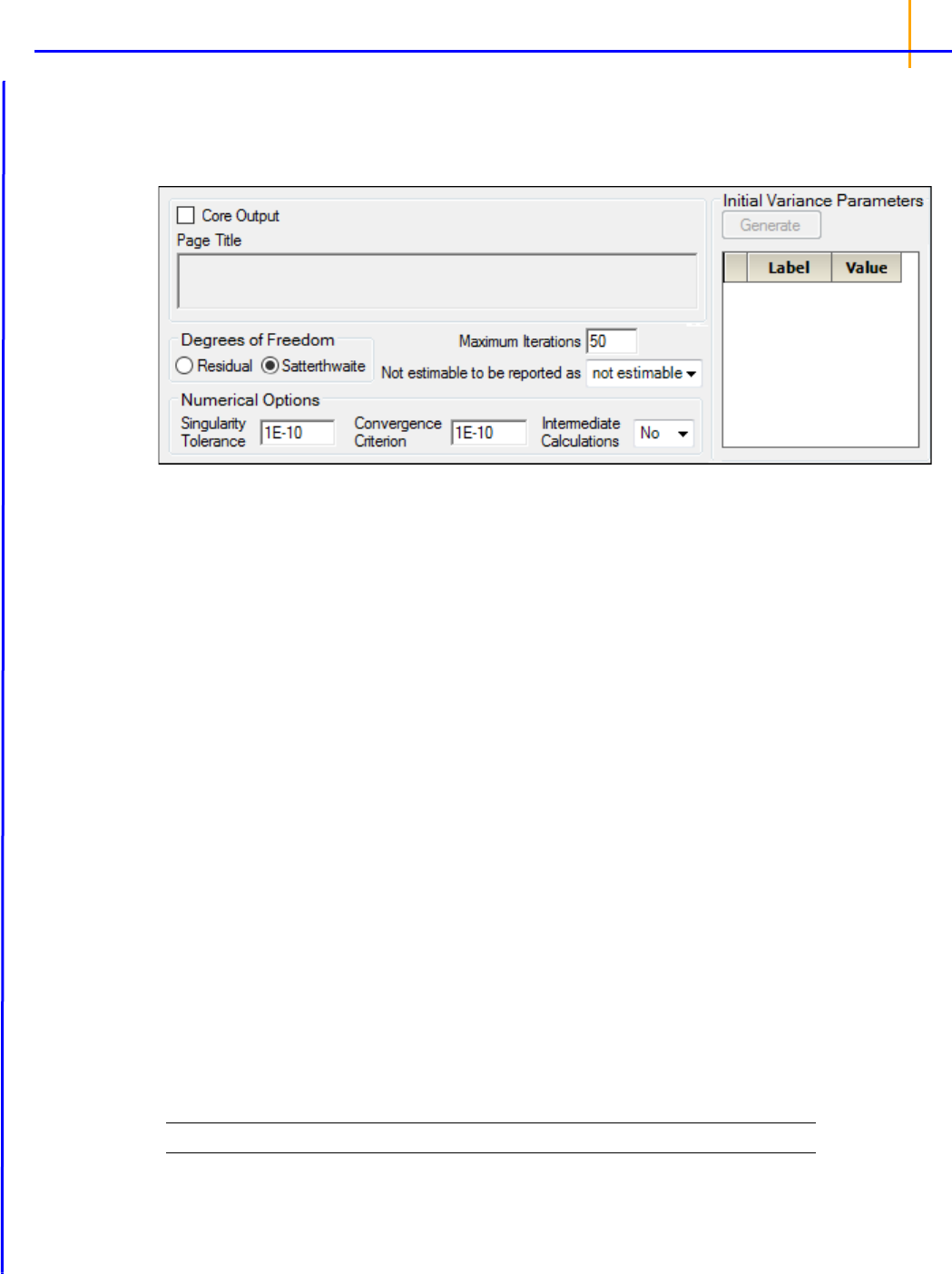
•Check the Core Output checkbox to include the Core Output text file in the results.

• In the Page Title field, type a title for the Core Output text file.

• Choose the degrees of freedom calculation method:

Residual: The same as the calculation method used in a purely fixed effects model.

Satterthwaite: The default setting and computes the df base on





approximation to distribution

of variance.

• In the Maximum Iterations field, type the number of maximum iterations. This is the number of

iterations in the Newton fitting algorithm. The default setting is 50.

• Use the Not estimable to be reported as menu to determine how output that is not estimable is

represented.

• not estimable

•0 (zero)

• In the Singularity Tolerance field, type the tolerance level. The columns in X and Z are elimi-

nated if their norm is less than or equal to this number. (Default tolerance value is 1E–10.)

• In the Convergence Criterion field, type the criterion used to determine if the model has con-

verged (default is 1E–10).

• In the Intermediate Calculations menu, select whether (Yes) or not (No) to include the design

matrix, reduced data matrix, asymptotic covariance matrix of variance parameters, Hessian, and

final variance matrix in the Core Output text file.

• In the Initial Variance Parameters group, click Generate to edit the initial variance parameters

values.

Note: The Generate initial variance parameters option is available only if the model uses random effects.

• Select a cell in the Value column and type a value for the parameter (default is 1).

If the values are not specified, then Phoenix uses the method of moments estimates.

Phoenix WinNonlin

User’s Guide



To delete one or more of the parameters from the table:

• Highlight the row(s).

•Select Edit >> Delete from the menubar or press X in the main toolbar.

• Click the Selected Row(s) option button and click OK.

Population/Individual bioequivalence options

• Select the Core Output checkbox to include the Core Output text file in the results.

• In the Page Title field, type a title for the Core Output text file.

Results

The Bioequivalence object creates several output worksheets. Each type of bioequivalence model

also creates a text file with model settings. If the Core Output checkbox is selected, then a Core Out-

put text file that contains model output is added to the results.

Average bioequivalence output

Population/Individual bioequivalence output

Text output

Ratios test

Average bioequivalence output

• Average Bioequivalence: Output from the bioequivalence analysis. Columns include:

Dependent: Input data column mapped to the Dependent context.

Units: Units, if specified in the input dataset.

FormVar: Input data column mapped to the Formulation context.

FormRef: Reference formulation.

RefLSM: Reference least squares mean.

RefLSM_SE: Standard error computed for reference least squares mean.

RefGeoLSM: Geometric reference least squares mean. 

Test: Test formulation.

TestLSM: Test least squares mean.

TestLSM_SE: Standard error computed for test least squares mean.

TestGeoLSM: Geometric test least squares mean. 

Difference: Difference between test and reference LSM values.

Diff_SE: Standard error of the difference in LSM values.

Diff_DF: Degrees of freedom for the difference in LSM values.

Ratio_%REF_: Percent ration of test LMS to reference LSM values.

(See

“Least squares means” for more details.)

CI_xx_Lower(Upper): Confidence interval computations. (See

“Classical intervals” for more

details.)

t1_TOST: Left-tail test result.

t2_TOST: Right-tail test result.

Prob_80(125)_00: Probability results for the two one-sided t-tests.

MaxProb: Largest value of the probability results.

TotalProb: Sum of the probability results. 

(See

“Two one-sided t-tests” for more details.)

Power_TOST: Power of the two one-sided t-tests. (See

“Power of the two one-sided t-tests proce-

dure”

for more details.)

AHpval: Anderson-Hauck test statistic. (See

“Anderson-Hauck test” for more details.)

Power_80_20: Power to detect a difference in least square means equal to 20% of the reference

LSM. (See

“Power for 80/20 Rule” for more details.)

Prob_Eq_Var: Probability of equal variance. (See

“Tests for equal variances” for more details.)

• Ratios Test: Ratios of reference to test mean computed. One worksheet for each test formula-

tion.

• User Settings: User-specified settings

For convenience, the Linear Mixed Effects Modeling output is also included with Average Bioequiva-

lence, but note that, since there is no specification of test or reference in Linear Mixed Effects Model-

ing, the LSM differences are computed alphabetically, which could correspond to reference minus test

formulation rather than test minus reference.

Phoenix WinNonlin

User’s Guide

• Diagnostics: Number of observations, number of observations used, residual sums of squares,

residual degrees of freedom, residual variance, restricted log likelihood, AIC, SBC, and Hessian

eigenvalues

• Final Fixed Parameters: Sort variables, dependent variable(s), units, effect level, parameter esti-

mate, t-statistic, p-value, intervals, etc.

• Final Variance Parameters: Final estimates of the variance parameters

• Initial Variance Parameters: Parameter and estimates for variance parameters

• Iteration History: Iteration, Obj_function, and column for each variance parameter

• Least Squares Means: Sort variable(s), dependent variable(s), units, and the least squares

means for the test formulation

• LSM Differences: Difference in least squares means

• Parameter Key: Variance parameter names assigned by Phoenix

• Partial SS: Only for 2x2 crossover designs using the default model: ANOVA sums of squares,

degrees of freedom, mean squares, F-tests and p-values for partial test

• Partial Tests: Sort Variable(s), Dependent Variable(s), Units, Hypothesis, Hypothesis degrees of

freedom, Denominator degrees of freedom, F statistic, and p-value

• Residuals: Sort Variable(s), Dependent Variable(s), Units, and information on residual effects vs.

predicted and observed effects

• Sequential SS: Only for 2x2 crossover designs using the default model: ANOVA sums of

squares, degrees of freedom, mean squares, F-tests and p-values for sequential test

• Sequential Tests: Sort Variable(s), Dependent Variable(s), Units, Hypothesis, Hypothesis

degrees of freedom, Denominator degrees of freedom, F statistic, and p-value

Population/Individual bioequivalence output

The worksheets that are created depend on which model options are selected.

• Population Individual: Output from the bioequivalence analysis. Columns include:

Dependent: Input data column mapped to the Dependent context.

Units: Units, if specified in the input dataset.

Statistic: Name of the statistic.

Value: Computed value of the statistic.

Upper_CI: Upper bound (an upper bound < 0 indicates bioequivalence).

Conclusion: Bioequivalence conclusion.

• Ratios Test: Ratios of reference to test mean. One worksheet for each test formulation.

• User Settings: User-specified settings

The population/individual bioequivalence statistics include:

Difference (Delta): Difference in sample means between the test and reference formulations.

Ratio(%Ref): Ratio of the test to reference means expressed as a percent. This is compared with

the percent of reference to detect that was specified by the user, to determine if bioequivalence

has been shown. The ratio is expected to be 100% if both formulations are exactly equal. If the

values of the two dependents are both over 100, it indicates that the test formulation resulted in

higher average exposure than the reference. Values <100 indicate the reverse. For example, if

the user specified a percent of reference to detect of 20%, and also specified a ln-transform, then

Ratio(%Ref) needs to be in the interval (80%, 125%) to show bioequivalence for the ratio test.

See “Least squares means” for more details.

SigmaR: value that is compared with sigmaP, the Total SD Standard, to determine whether mixed

scaling for population bioequivalence will use the constant-scaling values or the reference-scaling

values.

SigmaWR: value that is compared with sigmaI, the Within Subject SD Standard, to determine

whether mixed scaling for individual bioequivalence will use the constant-scaling values or the

reference-scaling values.

See “Bioequivalence criterion” for more details.

Com

puted bioequivalence statistics include:

Ref_Pop_eta: Test statistic for population bioequivalence with reference scaling

Const_Pop_eta: Test statistic for population bioequivalence with constant scaling

Mixed_Pop_eta: Test statistic for population bioequivalence with mixed scaling

Ref_Indiv_eta: Test statistic for individual bioequivalence with reference scaling

Const_Indiv_eta: Test statistic for individual bioequivalence with constant scaling

Mixed_Indiv_eta: Test statistic for individual bioequivalence with mixed scaling

Because population/individual bioequivalence only allows crossover designs, the output also contains

the ratios test, described under “Ratios test”.

Text output

The Bioequivalence object creates two types of text output: a Settings file that contains model set-

tings, and an optional Core Output file. The Core Output text file is created if the Core Output check-

box is selected in the General Options tab, then the Core Output text file is created. The file contains

a complete summary of the analysis, including all output as well as analysis settings and any errors

that occur.

Ratios test

ln_transform: test

ln

---------------









exp=

log10_transform: test 10

1–

log



For any bioequivalence study done using a crossover design, the output also includes for each test

formulation a table of differences and ratios of the original data computed individually for each sub-

ject.

Let

test be the value of the dependent variable measured after administration of the test formulation

for one subject. Let

ref be the corresponding value for the reference formulation, for the case in which

only one dependent variable measurement is made. If multiple test or reference values exist for the

same subject, then let

test be the mean of the values of the dependent variable measured after

administration of the test formulation, and similarly for

ref, except for the cases of ‘ln-transform’ and

‘log10-transform’ where the geometric mean should be used:

where

are the measurements after administration of the test formulation, and similarly for ref. For

each subject, for the cases of no transform, ln-transform, or log10-transform, the ratios table contains:

Phoenix WinNonlin

User’s Guide

Difference=test – ref



Ratio(%Ref)=100*test/ref

For data that was specified to be ‘already ln-transformed,’ these values are back-transformed to be in

terms of the original data:

Difference=exp(test) – exp(ref)



Ratio(%Ref)=100*exp(test – ref)=100*exp(test)/exp(ref)

Similarly, for data that was specified to be ‘already log10-transformed’:

Difference=10

test

– 10

ref



Ratio(%Ref)=100*10

test

– ref=100*10

test

/10

ref

Note: For ‘already transformed’ input data, if the mean is used for test or ref, and the antilog of test or

ref is taken above, then this is equal to the geometric mean.

Bioequivalence overview

Bioequivalence is said to exist when a test formulation has a bioavailability that is similar to that of

the reference. There are three types of bioequivalence: Average, Individual, and Population. Average

bioequivalence states that average bioavailability for test formulation is the same as for the reference

formulation. Population bioequivalence is meant to assess equivalence in prescribability and takes

into account both differences in mean bioavailability and in variability of bioavailability. Individual bio-

equivalence is meant to assess switchability of products, and is similar to population bioequivalence.

The US FDA Guidance for Industry (January 2001) recommends that a standard in vivo bioequiva-

lence study design be based on the administration of either single or multiple doses of the test and

reference products to healthy subjects on separate occasions, with random assignment to the two

possible sequences of drug product administration. Further, the 2001 guidance recommends that sta-

tistical analysis for pharmacokinetic parameters, such as area under the curve (AUC) and peak con-

centration (Cmax) be based on a test procedure termed the two one-sided tests procedure to

determine whether the average values for pharmacokinetic parameters were comparable for test and

reference formulations. This approach is termed average bioequivalence and involves the calculation

of a 90% confidence interval for the ratio of the averages of the test and reference products. To estab-

lish bioequivalence, the calculated interval should fall within a bioequivalence limit, usually 80–125%

for the ratio of the product averages. In addition to specifying this general approach, the 2001 guid-

ance also provides specific recommendations for (1) logarithmic transformations of pharmacokinetic

data, (2) methods to evaluate sequence effects, and (3) methods to evaluate outlier data.

It is also recommended that average bioequivalence be supplemented by population and individual

bioequivalence. Population and individual bioequivalence include comparisons of both the averages

and variances of the study measure. Population bioequivalence assesses the total variability of the

measure in the population. Individual bioequivalence assesses within-subject variability for the test

and reference products as well as the subject-by-formulation interaction.

Bioequivalence studies

Bioequivalence between two formulations of a drug product, sometimes referred to as relative bio-

availability, indicates that the two formulations are therapeutically equivalent and will provide the

same therapeutic effect. The objectives of a bioequivalence study is to determine whether bioequiva-

lence exists between a test formulation and reference formulation and to identify whether the two for-

mulations are pharmaceutical alternatives that can be used interchangeably to achieve the same

effect.

Bioequivalence studies are important because establishing bioequivalence with an already approved

drug product is a cost-efficient way of obtaining drug approval. Bioequivalence studies are also useful

for testing new formulations of a drug product, new routes of administration of a drug product, and for

a drug product that has changed after approval.

There are three different types of bioequivalence: average bioequivalence, population bioequiva-

lence, and individual bioequivalence. All types of bioequivalence comparisons are based on the cal-

culation of a criterion (or point estimate), on the calculation of an interval for the criterion, and on a

predetermined acceptability limit for the interval.

A procedure for establishing average bioequivalence involves administration of either single or multi-

ple doses of the test and reference formulations to subjects, with random assignment to the possible

sequences of drug administration. Then a statistical analysis of pharmacokinetic parameters such as

AUC and Cmax is done on a log-transformed scale to determine the difference in the average values

of these parameters between the test and reference data, and to determine the interval for the differ-

ence. To establish bioequivalence, the interval, usually calculated at the 90% level, should fall within a

predetermined acceptability limit, usually within 20% of the reference average. An equivalent

approach using two, one-sided t-tests is also recommended. Both the interval approach and the two

one-sided t-tests are described further below.

Phoenix WinNonlin

User’s Guide

The average bioequivalence should be supplemented by population and individual bioequivalences.

These added approaches are needed because average bioequivalence uses only a comparison of

averages, and not the variances, of the bioequivalence measures. In contrast, population and individ-

ual bioequivalence approaches include comparisons of both the averages and variances of the study

measure. The population bioequivalence approach assesses the total variability of the study measure

in the population. The individual bioequivalence approach assesses within-subject variability for the

test and reference products as well as the subject-by-formulation interaction.

The concepts of population and individual bioequivalence are related to two types of drug inter-

changeability: prescribability and switchability. Drug prescribability refers to when a physician pre-

scribes a drug product to a patient for the first time, and must choose from a number of bioequivalent

drug products. Drug prescribability is usually assessed by population bioequivalence. Drug switch-

ability refers to when a physician switches a patient from one drug product to a bioequivalent product,

such as when switching from an innovator drug product to a generic substitute within the same

patient. Drug switchability is usually assessed by individual bioequivalence.

Covariance structure types

The covariance types used in the Bioequivalence model object are the same as those used in the Lin-

ear Mixed Effects model object. For more on variance structures see

“Variance structure” in the Lin-

Mix section. Covariance types must be specified if the model contains random effects.

The Variance Structure tab in the Bioequivalence object allows users to select the covariance type

used in the model. The variances of the random-effects parameters become the covariance parame-

ters for a bioequivalence model that contains both fixed effect and random effect parameters.

The choices for covariance structures are listed below. The list uses the following notation:

n: number of groups. n=1 if the group option is not used. 

t: number of time points in the repeated context.

b: dimension parameter: for some variance structures, the number of bands; for others, the num-

ber of factors.

1(expression): 1 if the expression is true, 0 if the expression is false.

Variance Components have

n parameters; i

, j

element:



1(i = j)

i corresponds to k

effect

Unstructured has

n x t x (t + 1)/2 parameters; i

, j

element:



in output, 

= un(i,j)

Banded Unstructured (b) has n x b/2(2t – b +1) parameters, if b < t; otherwise, same as Unstruc-

tured; i

, j

element:



(|i – j| < n)

Compound Symmetry has

n x 2 parameters; i

, j

element:





+ 



1(i = j)

in output,





= csDiag, 



= csBlock

Heterogeneous Compound Symmetry has n x (t + 1) parameters; i

, j

element:

in output,



= cshSD(i),  = cshCorr



1 ij



1 ij=+

Autoregressive (1) has n x 2 parameters; i

, j

element:









i – j

in output,



= arVar,  = arCorr

Heterogeneous Autoregressive (1) has n x (t + 1) parameters; i

, j

element:







i – j

in output,



= arhSD(i),  = arhCorr

No-Diagonal Factor Analytic has n x t(t + 1)/2 parameters; i

, j

element:

in output,



= lambda(i,k)

Banded No-Diagonal Factor Analytic (b) has n x b/2(2t – b + 1) parameters if b < t; otherwise,

same as No-Diagonal Factor Analytic; i

, j

element:

in output,



= lambda(i,k)

Data limits and constraints

The limits and constraints discussed here are for Bioequivalence and Linear Mixed Effects modeling.

Cell data may not include question marks (?) or either single (') or double (“) quotation marks.

Variable names must begin with a letter. After the first character, valid characters include numbers

and underscores (my_file_2). They cannot include spaces or the following operational symbols: +, –,

*, /, =. They also cannot include parentheses (), question marks (?), semicolons (;), single or double

quotes.

Titles (in Contrasts, Estimates, or ASCII) can have single or double quotation marks, but not both.

The following are maximum counts for variables.

model terms 30

factors in a model term 10

sort keys 16

dependent variables 128

covariate/regressor variables 255

variables in the dataset 256

levels per variable 1,000

random and repeated statements 10

contrast statements 100

estimate statements 100

combined length of all variance parameter names (total characters) 10,000



k1=

min i j n









k1=

min i j b







Phoenix WinNonlin

User’s Guide

combined length of all level names (total characters) 10,000

combined length of input data line (total characters in line of data or column headers) 2,500

Average bioequivalence study designs

The most common designs for bioequivalence studies are replicated crossover, nonreplicated cross-

over, and parallel. In a parallel design, each subject receives only one formulation in randomized fash-

ion, whereas in a crossover design each subject receives different formulations in different time

periods. Crossover designs are further broken down into replicated and nonreplicated designs. In

nonreplicated designs, subjects receive only one dose of the test formulation and only one dose of the

reference formulation. Replicated designs involve multiple doses. A bioequivalence study should use

a crossover design unless a parallel or other design can be demonstrated to be more appropriate for

valid scientific reasons. Replicated crossover designs should be used for individual bioequivalence

studies, and can be used for average or population bioequivalence analysis.

An example of a nonreplicated crossover design is the standard 2x2 crossover design described

below.

Information about the following topics is available:

Recommended models for average bioequivalence

Least squares means

Classical intervals

Two one-sided t-tests

Power of the two one-sided t-tests procedure

Anderson-Hauck test

Power for 80

/20 Rule

Tests for equal variances

Recommended models for average bioequivalence

The default fixed effects, random effects, and repeated models for average bioequivalence studies

depends on the type of study design: replicated crossover, nonreplicated crossover, or parallel.

Replicated crossover designs

Replicated data is defined as data for which, for each formulation, there exists at least one subject

with more than one observation of that formulation. The default models depend on the type of analy-

ses and the main mappings. For replicated crossover designs, the default model used in the Bioequiv-

alence object is as follows:

Fixed effects model: Sequence + Formulation + Period

Random effects model: Subject(Sequence) and Type: Variance Components

Repeated specification: Period

Variance Blocking Variables: Subject

Group: Treatment

Type: Variance Components

Phoenix WinNonlin

User’s Guide

Nonreplicated crossover designs

Nonreplicated data is defined as data for which there exists at least one formulation where every sub-

ject has only one observation of that formulation. The default models depend on the type of analyses,

the main mappings, and a preference called Default for 2x2 crossover set to all fixed effects (set

under Edit > Preferences > LinMixBioequivalence). For nonreplicated crossover designs, the

default model is as follows.

Fixed effects model: Sequence + Formulation + Period

Unless the bioequivalence preference Default for 2x2 crossover set to all fixed effects is

turned on in the Preferences dialog (Edit > Preferences > LinMixBioequivalence), in which

case the model is Sequence + Subject(Sequence) + Formulation + Period.

Random effects model: Subject(Sequence) and Type: Variance Components

Unless the bioequivalence preference Default for 2x2 crossover set to all fixed effects is

turned on, in which case the model is not specified (the field is empty).

Repeated model is not specified.

Since there is no repeated specification, the default error model

 ~ N(0, 

I) is used. This is equiva-

lent to the classical analysis method, but using maximum likelihood instead of method of moments to

estimate inter-subject variance. Using Subject as a random effect this way, the correct standard errors

will be computed for sequence means and tests of sequence effects. Using a fixed effect model, one

must construct pseudo-F tests by hand to accomplish the same task.

Note: If Warning 11094 occurs, “Negative final variance component. Consider omitting this VC struc-

ture.”, when Subject(Sequence) is used as a random effect, this most likely indicates that the

within-subject variance (residual) is greater than the between-subject variance, and a more appro-

priate model would be to move Subject(Sequence) from the random effects to the fixed effects

model, i.e., Sequence+Subject(Sequence)+Formulation + Period.

When this default model is used for a standard 2x2 crossover design, Phoenix creates two additional

worksheets in the output called Sequential SS and Partial SS, which contain the degrees of freedom

(DF), Sum of Squares (SS), Mean Squares (MS), F-statistic and p-value, for each of the model terms.

These tables are also included in the text output. Note that the F-statistic and p-value for the

Sequence term are using the correct error term since Subject(Sequence) is a random effect.

If the default model is used for 2x2 and the data is not transformed, the

intrasubject CV parameter is

added to the Final Variance Parameters worksheet:

intrasubject CV=sqrt(Var(Residual))/RefLSM

where

RefLSM is the Least Squares Mean of the reference treatment.

If the default model is used for 2x2 and the data is

either ln-transformed or log10-transformed, the

intra-su

bject CV and intrasubject CV parameters are added to the Final Variance Parameters

work

-sheet:

For ln-transformed data:

intersubject CV=sqrt(exp(Va r(Sequence*Subject)) – 1)

intrasubject CV=sqrt(exp(Residual) – 1)

For log10-transformed data:

intersubject CV=sqrt(10^(ln(10)*Var (Sequence*Subject)) – 1)

intrasubject CV=sqrt(10^(ln(10)*Var (Residual)) – 1)

Note that for this default model Var (Sequence*Subject) is the intersubject (between subject) vari-

ance, and

Residual is the intrasubject (within subject) variance.

Parallel designs

For parallel designs, whether data is replicated or nonreplicated, the default model is as follows.

Fixed effects model: Formulation

There is no random model and no repeated specification, so the residual error term is included in the

model.

Note: In each case, users can supplement or modify the model to suit the analysis needs of the dataset.

For example, if a Subject effect is appropriate for the Parallel option, as in a paired design (each

subject receives the same formulation initially and then the other formulation after a washout

period), set the Fixed Effects model to Subject+Formulation.

Note: When mapping a new input dataset to a Bioequivalence object, if the mappings are identical for

the new mapped dataset, then the model will remain the same. If there are any mapping changes

other than mapping an additional dependent variable, then the model will be rebuilt to the default

model since the existing model will not be valid anymore. This occurs for mapping changes either

made by the user or made automatically due to different column names in the dataset matching

the mapping context.



The user can reset to the default model at any time by making any mapping change, such as

unmapping and remapping a column.

Least squares means

In determining the bioequivalence of a test formulation and a reference formulation, the first step is

the computation of the least squares means (LSM) and standard errors of the test and reference for-

mulations and the standard error of the difference of the test and reference least squares means.

These quantities are computed by the same process that is used for the Linear Mixed Effects module.

See “Least squares means” in the LinMix section.

o simplify the notation for this and the following sections, let:

RefLSM: reference least squares mean,

TestLSM: test least squares mean,

fractionToDetect: (user-specified percent of reference to detect)/100,

DiffSE: standard error of the difference in LSM,

RatioSE: standard error of the ratio of the least squares means,

df: degrees of freedom for the difference in LSM.

The geometric LSM are computed for transformed data. For ln-transform or data already ln-trans-

formed,

RefGeoLSM = exp(RefLSM) 

TestGeoLSM = exp(TestLSM)

For log10-transform or data already log10-transformed,

RefGeoLSM = 10

RefLSM



TestGeoLSM = 10

TestLSM

Phoenix WinNonlin

User’s Guide

The difference is the test LSM minus the reference LSM,

Difference = TestLSM – RefLSM

The ratio calculation depends on data transformation. For non-transformed,

For ln-transform or data already ln-transformed, the ratio is obtained on arithmetic scale by exponen-

tiating,

Ratio(%Ref) = 100exp(Difference)

Similarly for log10-transform or data already log10-transformed, the ratio is

Ratio(%Ref) = 100 x 10

Difference

Classical intervals

Output from the Bioequivalence module includes the classical intervals for confidence levels equal to

80, 90, 95, and for the confidence level that the user gave on the Options tab if that value is different

than 80, 90, or 95. To compute the intervals, first the following values are computed using the

students-t distribution, where 2*alpha=(100 – Confidence Level)/100, and Confidence Level is

specified in the user inter-face.

These values are included in the output for the no-transform case. These values are then transformed

if necessary to be on the arithmetic scale, and translated to percentages. For ln-transform or data

already ln-transformed,

CI_Lower = 100exp(Lower) 

CI_Upper = 100exp(Upper)

For log10-transform or data already log10-transformed,

CI_Lower = 100 x 10

Lower



CI_Upper = 100 x 10

Upper

For no transform,



= 

where the approximation

RatioSE=DiffSE/RefLSM is used. Similarly,

Ratio %Ref100

TestLSM

RefLSM

-----------------------





Lower t

1 – df(,)

DiffSE

Upper Difference t

1 – df(,)

DiffSE+

CI_Lower 100 1

Lower

RefLSM

---------------------





100 1

TestLSM RefLSM–

RefLSM

--------------------------------------------------





1 – df(,)



DiffSE

RefLSM

---------------------

–+





100

TestLSM

RefLSM

-----------------------

1 – df(,)

RatioSE–





Con

cluding whether bioequivalence is shown depends on the user-specified values for the level and

for the percent of reference to detect. These options are set on the Options tab in the Bioequivalence

object. To conclude whether bioequivalence has been achieved, the

CI_Lower and CI_Upper for

the user-specified value of the level are compared to the following lower and upper bounds. Note that

the upper bound for log10 or ln-transforms or for data already transformed is adjusted so that the

bounds are symmetric on a logarithmic scale.

LowerBound



= 100 – (percentReferenceToDetect)

UpperBound (ln-transforms) 

= 100 exp(–ln(1 –

fractionToDetect))

= 100 (1/(1 –

fractionToDetect))

UpperBound (log10-transforms) 

= 100*10^(–log10(1 –

fractionToDetect))

= 100 (1/(1 –

fractionToDetect))

UpperBound (no transform) 

= 100+(

percentReferenceToDetect)

If the interval (

CI_Lower, CI_Upper) is contained within LowerBound and UpperBound, average

bioequivalence has been shown. If the interval (

CI_Lower, CI_Upper) is completely outside the

interval (

LowerBound, UpperBound), average bioinequivalence has been shown. Otherwise, the

module has failed to show bioequivalence or bioinequivalence.

Two one-sided t-tests

For ln-transform or data already ln-transformed, the first t-test is a left-tail test of the hypotheses:

: trueDifference < ln(1 – fractionToDetect) (bioinequivLeftTest)

: trueDifference  ln(1 – fractionToDetect) (bioequivLeftTest)

The test statistic for performing this test is:

=((TestLSM – RefLSM) – ln(1 – fractionToDetect))/DiffSE

The p-value is determined using the t-distribution for this t-value and the degrees of freedom. If the p-

value is <0.05, then the user can reject

at the 5% level, i.e. less than a 5% chance of rejecting H

when it was actually true.

For log10-transform or data already log10-transformed, the first test is done similarly using log10

instead of ln.

For data with no transformation, the first test is (where Ratio here refers to the true ratio of the Test

mean to the Reference mean):

: Ratio < 1 – fractionToDetect



: Ratio  1 – fractionToDetect

The test statistic for performing this test is:

=[(TestLSM/RefLSM) – (1 – fractionToDetect)]/RatioSE

CI_Upper 100 1

Upper

RefLSM

---------------------





Phoenix WinNonlin

User’s Guide

where the approximation RatioSE=DiffSE/RefLSM is used.

The second t-test is a right-tail test that is a symmetric test to the first. However for log

or ln-trans-

forms, the test will be symmetric on a logarithmic scale. For example, if the percent of reference to

detect is 20%, then the left-tail test is Pr(<80%), but for ln-transformed data, the right-tail test is

Prob(>125%), since ln(0.8) = –ln(1.25).

For ln-transform or data already ln-transformed, the second test is a right-tail test of the hypotheses:

: trueDifference > –ln(1 – fractionToDetect) (bioinequivRightTest)

: trueDifference  –ln(1 – fractionToDetect) (bioequivRightTest)

The test statistic for performing this test is:

=((TestLSM – RefLSM)+ln(1 – fractionToDetect))/DiffSE

For log10-transform or data already log10-transformed, the second test is done similarly using log

instead of ln.

For data with no transformation, the second test is:

: Ratio > 1+fractionToDetect



: Ratio  1+fractionToDetect

The test statistic for performing this test is:

=((TestLSM/RefLSM) – (1+fractionToDetect))/RatioSE

where the approximation RatioSE=DiffSE/RefLSM is used.

The output for the two one-sided t-tests includes the

and t

values described above, the p-value for

the first test described above, the p-value for the second test above, the maximum of these p-values,

and total of these p-values. The two one-sided t-tests procedure is operationally equivalent to the

classical interval approach. That is, if the classical (1 – 2 x alpha) x100% confidence interval for differ-

ence or ratio is within LowerBound and UpperBound, then both the

s given above for the two tests

are also rejected at the alpha level by the two one-sided t-tests.

Power of the two one-sided t-tests procedure

Power_TOST in the output is the power of the two one-sided t-tests procedure described in the previ-

ous section. Refer to the previous section for the definitions of t

and t

for the transformation that was

used and recall from previous sections that df is the degrees of freedom for the difference of the test

and reference least squares means. Define the critical t-value as:

where 2

=(100 – Confidence Level/100) and Confidence Level is specified in the user interface.

In general:

PowerOfTest=1 – (probTypeIIError) = probRejectingH

, when H

is true

For the two one-sided t-tests procedure, H

is bioequivalence (concluded when both of the one-sided

tests pass) and H

is nonequivalence. The power of the two one-sided t-tests procedure is (Phillips,

K. F. (1990), or Diletti, E., Hauschke, D., and Steinijans, V. W. (1991)):

Power = Prob{t

 t

crit

and t

 –t

crit

| bioequivalence}

crit

1 –df,

– 



+–2

DiffSE

---------------------------------------------------------

This power is closely approximated by the difference of values from a non-central t-distribution

(Owen, D. B. (1965)):

Power_TOST = p(–t

crit

,df,t

) – p(t

crit

,df,t

)

This is the formula used in the Bioequivalence module (power is set to zero if this results in a nega-

tive), and the non-central t should be accurate to 1e–8. If it fails to achieve this accuracy, the non-cen-

tral t-distribution is approximated by a shifted central t-distribution (again, power is set to zero if this

results in a negative):

Power_TOST = p(–t

crit

,–t

,df) – p(t

crit

,–t

,df)

Power of the two one-sided t-tests procedure is more likely to be of use with simulated data, such as

when planning for sample size, rather than for drawing conclusions for observed data.

Anderson-Hauck test

See Anderson and Hauck (1983), or page 99 of Chow and Liu (2000). Briefly, the Anderson-Hauck

test is based on the hypotheses:

: 

– 

< 

vs H

: 

– 

> 

: 

– 

< 

vs H

: 

– 

> 

where



and 

are the natural logarithm of the Anderson-Hauck limits entered in the bioequiva-

lence options tab. Rejection of both null hypotheses implies bioequivalence. The Anderson-

Hauck test statistic is

given by:

where DiffSE is the standard error of the difference in means. Under the null hypothesis, this test

statistic has a noncentral t-distribution.

Power for 80/20 Rule

Power_80_20 in the output is the power to detect a difference in least square means equal to 20% of

the reference least squares mean. Percent of Reference to Detect on the Options tab should be the

default value of 20%, and the desired result is that Power_80_20 is greater than 0.8 or 80%. (See pg.

142–143 of Chow and Liu (2000).) In general:

PowerOfTest=1 – (probTypeIIError) = probRejectingH

, when H

is true

Let





and 

be the true (not observed) values of TestLSM and RefLSM. For this type of power cal-

culation, for the no-transform case, the power is the probability of rejecting:

(

T =



) given H



– 

| = fractionToDetect(

)

For ln-transform, and data already ln-transformed, this changes to:



= –

| = –ln(1– fractionToDetect)

and similarly for log10-transform and data already log10-transformed.

For the default

fractionToDetect=0.2, the default =0.05 (2*=(100 – Confidence_Level) /100),

with no transform on the data and



> 0:

Phoenix WinNonlin

User’s Guide

Power = Pr

(rejecting

at the alpha level given the true difference in means = 0.2 x 

)

given |



– 

| = 0.2(

)

Let:

Then:

Power  1 – [Pr(T > t

) – Pr(T > t

)]

where

T has a central t distribution with df=Diff_DF. Note that the second probability may be neg-

ligible.

For ln-transform or data already ln-transformed, this changes to:

Tests for equal variances

For the default parallel and 2x2 crossover models, some tests in Bioequivalence (e.g., the two one-

sided t-tests) rely on the assumption that the observations for the group receiving the test formulation

and the group receiving the reference formulation come from distributions that have equal variances,

in order for the test statistics to follow a t-distribution. There are two tests in Bioequivalence that verify

whether the assumption of equal variances is valid:

The Levene test is done for a parallel design that uses the default model (formulation variable

with intercept included). See Snedecor and Cochran (1989) for more information.

The Pitman-Morgan test is done for a 2-period, 2-sequence, 2-formulation crossover design that

uses either Variance Components or all fixed effects model. See Chow and Liu (2nd ed. 2000 or

3rd ed. 2009) for more information. In addition to the required column mappings, Sequence and

Period must also be mapped columns.

For replicated crossover designs, the default model in Bioequivalence already adjusts for unequal

variances by using Satterthwaite Degrees of Freedom and by grouping on the formulation in the

repeated model, so a test for equality of variances is not done.

The results of the Levene test and Pitman-Morgan test are given in the Average Bioequivalence out-

put worksheet and at the end of the Core Output. Both tests verify the null hypothesis that the true

variances for the two formulations are equal by using the sample data to compute an F-distributed

TestLSM RefLSM–

DiffSE

--------------------------------------------------

 df(, )



1 – df(,)

0.2

RefLSM

DiffSE

---------------------





–

t–

1 – df(,)

0.2

RefLSM

DiffSE

---------------------





–

1 – df(,)

0.8ln–

DiffSE

---------------------





–

t–

1 – df(,)

0.8ln–

DiffSE

---------------------





–

test statistic. A p-value of less than 0.05 indicates a rejection of the null hypotheses (and acceptance

that the variances are unequal) at the 5% level of significance.

If unequal variances are indicated by the Levene or Pitman-Morgan tests, the model can be adjusted

to account for unequal variances by using Satterthwaite Degrees of Freedom on the General Options

tab and using a ‘repeated’ term that groups on the formulation variable as follows.

For a parallel design:

• Map the formulation variable as Formulation.

• Use the default Fixed Effects model (the formulation variable).

• Use the default Degrees of Freedom setting of Satterthwaite

•

Map the Dependent variable, and map the Subject and Period variables as Classification vari-

ables. 



the data does not contain a Period column, a column that contains all ones can be added as the

Period variable.

• Set up the Repeated sub-tab of the Variance Structure tab as:

Repeated Specification: Period 

Variance Blocking Variables (Subject): Subject 

Group: Formulation

Type: Variance Components

For a 2x2 crossover design:

• Map the Sequence, Subject, Period, Formulation, and Dependent variables accordingly.

• Use the default model (Fixed Effects is Sequence+Formulation+Period, Random is Sub-

ject(Sequence)).

• Use the default Degrees of Freedom setting of Satterthwaite.

• Set up the Repeated sub-tab of the Variance Structure tab as:

Repeated Specification: Period

Variance Blocking Variables (Subject): Subject 

Group: Formulation

Type: Variance Components

Phoenix WinNonlin

User’s Guide

Population and individual bioequivalence

Population and individual bioequivalence are used to assess switchability and prescribability.

Because individual bioequivalence relies on estimates of within-subject, within-formulation variation,

replicated crossover designs are required. This algorithm was developed by Francis Hsuan. Designs

that can be appropriately analyzed include, but are not limited to the following list, which shows the

Sequence (Period) Design.

2 (4) TRTR/RTRT

4 (4) TRTR/RTRT/TRRT/RTTR 

4 (2) TT/RR/TR/RT 

4 (3) TRT/RTR/TRR/RTT 

2 (5) TRRTT/RTTRR 

3 (3) TRR/RTR/RRT

2 (3) RTR/TRT

6 (3) TRR/RTT/TRT/RTR/TTR/RRT

2 (4) TRRR/RTTT

6 (4) TTRR/RRTT/TRRT/RTTR/TRRR/RTTT

The algorithm works for balanced and unbalanced data with an equal number of periods in each

sequence and one measurement per subject in each period.

Bioequivalence criterion

Computational details

Bioequivalence criterion

Population bioequivalence (PBE) criteria are:

j'R

–

j'R

–

–

---

j'R

–

----------------------------------------------------------------------------



, if







j'R

–

E– Y

j'R

–

---



----------------------------------------------------------------------------



, if











–





+



–+ 0, if







–





–



–+0, if





=



=

where 

defaults to 0.2 and 

=(ln(1 – PercentReference)+

) /

. The default value for Per-

centReference is 0.20. In the Bioequivalence object,



is called the Total SD standard. 

computed by the program and is the total variance of the reference formulation, i.e., the sum of

within- and between-subject variance. The criteria take the linearized form:

–

j'R

–

–

---

j'R

–

---------------------------------------------------------------------------



, if



–

j'R

–

–

---



---------------------------------------------------------------------------



, if















–





+



–+ + 0, if



and





–





–



–++ 0, if=



where 

will be defined below.





=

Individual bioequivalence (IBE) criteria are:

where 

defaults to 0.2 and 

=(ln(1 – PercentReference)+

) /

. The default value for Percent

Reference is 0.20, and the default value for



is 0.05. In the Bioequivalence object, 

is called the

within-subject SD standard.



is computed by Phoenix, and its square, 

, is the within-sub-

ject variance of the reference formulation.

The IBE criteria take the linearized form:

For reference scaling, use



or 

. For constant scaling, use 

or 

. For mixed scaling, use one

of the following.

Population



> 

, use 





 

, use 

Individual



> 

, use







 

, use 

If the upper bound on the appropriate

 is less than zero, then the product is bioequivalent in the cho-

sen sense. The interval is set in the Bioequivalence object’s Options tab. The method of calculating

that upper bound follows.

Computational details

Let:

ijkt

be the response of subject j in sequence i at time t with treatment k.

be a vector of responses for subject

j in sequence i. The components of Y are arranged in

the ascending order of time. 

.be the design vector of treatment

T in sequence i.



Phoenix WinNonlin

User’s Guide

be a design vector for treatment R in sequence i.



> 1 be the number of subjects in sequence i.

Assume the mean responses of , follow a linear model:

where



, 

are the population mean responses of Y with treatments T and R respectively, and

are design/model matrices.

Let:

be the number of occasions

T is assigned to the subjects in sequence i.

be the number of occasions R is assigned to the subjects in sequence i.

Then:

Assume that the covariances:

follow the model:

where the parameters:

are defined as follows:



:= sum Z



:= sum Z



: p

1–

: p

1–

: u

–

and d

: s

1–

–=

ijkt

ijk't'

(, )





diag Z



diag Z





+



,,,{, }=



+= is varY

ijTt



+= is varY

ijRt

intra-subject correlation coefficients are:

intra-subject covariances are:

intra-subject variances are:

For PBE and IBE investigations, it is useful to define additional parameters:

Except for



, all the quantities above are non-negative when they exist. It satisfies the equation:

In general, this



may be negative. This method for PBE/IBE is based on the multivariate model.

This method is applicable to a variety of higher-order two-treatment crossover designs including TR/

RT/TT/RR (the Balaam Design), TRT/RTR, or TxRR/xRTT/RTxx/TRxx/xTRR/RxTT (Table 5.7 of

Jones and Kenward, page 205).





= is corr Y

T '

(, ), 1



0





= is corr Y

R '

(, ), 1



0





 is corr Y

(,), 1



1–=















is var Y

T '

–2



is var Y

R '

–2–=

–=



2



1 p

1–

–

–=



1 p

1–

–

–=



1–



1–



++=

–+=

var Y

ijT

ijR

–



++=

Phoenix WinNonlin

User’s Guide

Given the i

sequence, let:

where: 

is the sample mean of the

sequence.

is the within-sequence sample covariance matrix.

It can be shown that:

Furthermore, it can be shown that {

, S

} (for PBE) are statistically independent from {} and {S

iWT

iWR

}, and that the four statistics , S

, S

iWT

, S

iWR

(for IBE) are statistically independent.

Let



be sets of normalized weights, chosen to yield the method of moments estimates of the . Then

define the estimators of the components of the linearized criterion by:



i•



=, S

=

iWT

1 p

1–

–

1–

tr diag u

V

u'

–=

iWR

1 p

1–

–

1–

tr diag u

V

u'

–=

i•





– n

1–



(, )



1–

1–



1–



1–

1–



1–



1–

1–



1–

iWT



1–

1–

1–

1–



1–n

1–

iWR



1–

1–

1–

1–



1–n

1–



Using the above notation, one may define unbiased moment estimators for the PBE criteria:

and for the IBE criteria:







1 

1–



–









iWT





1 

1–



–









iWR





1 

1–



–









iWT

I3a

1 



1–











iWR

I3b



1 

1–











iWR









+E



+





– E

–





–++=

––++=





I3a





I3b

–





–++=





–++=

Phoenix WinNonlin

User’s Guide

Construct a 95% upper bound for  based on the TRTR/RTRT design using Howe’s approximation I

and a modification proposed by Hyslop, Hsuan and Holder (2000). This can be generalized to com-

pute the following sets of

, H, and U statistics:

where the degrees of freedom

are computed using Satterthwaite’s approximation. Then, the 95%

upper bound for each

is:

< 0, that indicates bioequivalence; H

 0 fails to show bioequivalence.

References

Anderson and Hauck (1983). A new procedure for testing equivalence in comparative bioavailability

and other clinical trials. Commun Stat Theory Methods, 12:2663–92.

Chow and Liu (2nd ed. 2000 or 3rd ed. 2009). Design and Analysis of Bioavailability and Bioequiva-

lence Studies, Marcel Dekker, Inc.

Hauschke, Steinijans, Diletti, Schall, Luus, Elze and Blume (1994). Presentation of the intrasubject

coefficient of variation for sample size planning in bioequivalence studies. Int J Clin Pharm Ther

32(7): 376–378.

Hyslop, Hsuan and Holder (2000). A small sample on interval approach to assess individual bioequiv-

alence. Statist Medicine 19:2885–97.

Schuirmann (1987). A comparison of the two one-sided tests procedure and the power approach for

assessing the equivalence of average bioavailability. J Pharmacokinet Biopharm 15:657–680.

Snedecor and Cochran (1989). Statistical Methods, 8th edition, Iowa State Press.

US FDA Guidance for Industry (March 2003). Bioavailability and Bioequivalence Studies for Orally

Administered Drug Products—General Considerations.

US FDA Guidance for Industry (January 2001). Statistical Approaches to Establishing Bioequiva-

lence.



.95,n

var





12







.05,n







for q= P1 P2 I1 I2



.95,



for q=

,,,

P3 P4 I3aI3b

,,,

–

for all q









12



+

for q=

P3 P4

for all other q

Phillips, K. F. (1990). Power of the Two One-Sided Tests Procedure in Bioequivalence. Journal of

Pharmacokinetics and Biopharmaceutics 18: 137–144.

Diletti, E., Hauschke, D., and Steinijans, V. W. (1991). Sample size determination for bioequivalence

assessment by means of intervals. Int. J. of Clinical Pharmacology, Therapy and Toxicology 29: 1–8.

Owen, D. B. (1965). A Special case of a bivariate noncentral t-distribution. Biometrika 52: 437–446.

Phoenix WinNonlin

User’s Guide

Bioequivalence model examples

Knowledge of how to do basic tasks using the Phoenix interface, such as creating a project and

importing data, is assumed.

Analyzing average bioequivalence of 2x2 crossover study example

Analyzing average bioequivalence of a replicated crossover design example

Evaluating individual and population bioequivalence example

Analyzing average bioequivalence of 2x2 crossover study example

The objective of this study is to compare a newly developed tablet formulation to the capsule formula-

tion that was being used in Phase II studies. Both had a label claim of 25 mg per dosing unit.

A 2x2 crossover design was chosen for this study. Twenty subjects were randomly assigned to one of

two sequence groups. Within each sequence group, each subject took both formulations, with a

washout period between. Drug concentrations in plasma were measured, and the AUClast (area

under a curve computed to the last observation) was calculated.

Data for this example are provided in

…\Examples\WinNonlin\Supporting files. The

dataset used is

Data 2x2.CSV.

The completed project (

Bioequivalence_2x2.phxproj) is available for reference in

…\Examples\WinNonlin.

Set up the object

Create a new project named Bioequivalence_2x2.

2. Import the file …\Examples\WinNonlin\Supporting files\Data 2x2.CSV.

3. Right-click Data 2x2 in the Data folder and then select Send To > Computation Tools > Bio-

equivalence.

4. In the Main Mappings panel:

Leave Sequence mapped to the Sequence context.

Leave Subject mapped to the Subject context.

Leave Period mapped to the Period context.

Leave Formulation mapped to the Formulation context.

Map AUClast to the Dependent context.

5. In the Model tab below the Setup panel, make sure that: 

Crossover is selected as the Type of study, 

Average is selected as the Type of Bioequivalence, and 

Capsule is selected as the Reference Formulation.

6. Select the Fixed Effects tab, make sure that:

Sequence+Formulation+Period appears in the Model Specification field. 

Ln(x) is selected in the Dependent Variables Transformation menu.

7. Select the Variance Structure tab.



The random effects are already specified in the Variance Structure tab. If they are not, type

Sub-

ject(Sequence)

in the Random Effects Model field.

Execute and view the results

Click (Execute icon) to execute the object. 



The Average Bioequivalence worksheet indicates that the difference in ln(AUClast) between for-

mulations is 0.046±0.073 (Difference±Diff_SE). The 90% confidence interval for the ratio is 92.216

(CI_90_Lower) to 118.780 (CI_90_Upper).



Since the interval is completely contained between 80 and 125, one can conclude that the formu-

lations are bioequivalent.

2. Select the Partial Tests worksheet and compare with the Sequential Tests worksheet.



Because the data are balanced, the sequential and partial tests are identical. Note that, in the

tests, Sequence is statistically significant, but no other factor is.



Select any cell with a numerical value in the Bioequivalence worksheet output and look in the

value display bar above to see the full precision of 15 decimal places.

Figure 8-1. Sequential Tests worksheet for 2x2 crossover study

This concludes the Bioequivalence example of analyzing a 2x2 crossover study.

Analyzing average bioequivalence of a replicated crossover design example

The objective of this study is to compare a newly developed tablet formulation to a capsule formula-

tion that was used in Phase II studies. Both formulations have the same label claim per dosing unit.

A RTRT/TRTR replicated crossover design was chosen for this study. Twenty subjects were randomly

assigned to one of two sequence groups. Concentrations of the drug were measured in plasma, and

the AUClast (area under the time-concentration curve, computed to the last observation) was calcu-

lated.

Note: The completed project (Bioequivalence_replicated.phxproj) is available for refer-

ence in …\Examples\WinNonlin.

Phoenix WinNonlin

User’s Guide

Set up the object

Create a project called Bioequivalence_replicated.

2. Import the file …\Examples\WinNonlin\Supporting files\Data 2x4.CSV.

1. Right-click Data 2x4 in the Data folder and select Send To > Computation Tools > Bioequiva-

lence.

2. In the Mappings panel:

Leave Sequence mapped to the Sequence context.

Leave Subject mapped to the Subject context.

Leave Period mapped to the Period context.

Leave Formulation mapped to the Formulation context.

Map AUClast to the Dependent context.

3. In the Model tab below the Setup panel, make sure that:

Crossover is selected as the Type of study, 

Average is selected as the Type of Bioequivalence, and 

Capsule is selected as the Reference Formulation.

4. Select the Fixed Effects tab and make sure that:

Sequence+Formulation+Period appears in the Model Specification field.

Ln(x) is selected in the Dependent Variables Transformation menu.

Note: Phoenix has automatically selected a model specification and classification variables based on the

model for replicated crossovers.

5. Select the Variance Structure tab.



Notice that the default variance structure for a replicated crossover design is substantially different

from and more complex than that for the 2x2 crossover design. As a result, the model fitting is

more difficult as well.



In the Random 1 sub-tab, make sure that:

Formulation appears in the Random Effects Model field.

Subject appears in the Variance Blocking Variables field. 

Banded No-Diagonal Factor Analytic(f) is selected in the Type menu.

2 is specified as the Number of factors.



In the Repeated sub-tab, make sure that:

Period appears in the Repeated Specification field.

Subject appears in the Variance Blocking Variables field.

Formulation appears in the Group field.

Variance Components is selected in the Type menu.

Execute and view the results

A user can expect that about 50% of datasets analyzed will produce a non-positive definite G matrix.

This does not imply that the model-fitting is invalid, but only that a user must be careful not to over-

interpret the variance estimates. The interval on the formulation difference will still have the expected

statistical properties.

1. Execute the object.



The Average Bioequivalence worksheet indicates that the analysis just failed to show bioequiva-

lence since the 90% confidence interval=91.612 (CI_90_Lower) and 125.772 (CI_90_Upper).

2. Select the Partial Tests worksheet and compare with the Sequential Tests worksheet.



Because the data are balanced, the sequential and partial tests are identical.

Figure 8-2. Partial Tests worksheet for replicated crossover study

Figure 8-3. Sequential Tests worksheet for replicated crossover study

This concludes the Bioequivalence example of analyzing a replicated crossover study.

Evaluating individual and population bioequivalence example

Phoenix can handle a wide variety of model designs suitable for assessing individual and population

bioequivalence, including:

TRTR/RTRT/TRRT/RTTR 

TT/RR/TR/RT 

TRT/RTR/TRR/RTT 

TRRTT/RTTRR 

TRR/RTR/RRT

RTR/TRT

TRR/RTT/TRT/RTR/TTR/RRT

TRRR/RTTT

TTRR/RRTT/TRRT/RTTR/TRRR/RTTT

where T=Test formulation and R=Reference formulation.

Note: Each sequence must contain the same number of periods. For each period, each subject must

have one measurement.

A bioequivalence example, included as part of

“Testing the Phoenix installation”, shows results for a

RTR/TRT design. This example demonstrates an analysis of a TT/RR/TR/RT design.

Note: The completed project (Bioequivalence_IndPop.phxproj) is available for reference in

…\Examples\WinNonlin.

Phoenix WinNonlin

User’s Guide

Set up the population/individual model

Create a project called Bioequivalence_IndPop.

2. Import the file …\Examples\WinNonlin\Supporting files\TT RR RT TR.DAT.



Notice that the number of subjects is not the same in each sequence group. TT, RR, TR, and RT

each have 4 subjects, whereas RT has 5.

3. Right-click TT RR RT TR in the Data folder and select Send To > Computation Tools > Bio-

equivalence.

4. In the Model tab below the Setup panel, select the Population/Individual option button in the

Type of Bioequivalence area.

5. Map the data types to the following contexts:

Leave Sequence mapped to the Sequence context.

Leave Subject mapped to the Subject context.

Leave Period mapped to the Period context.

Leave Formulation mapped to the Formulation context.

Map AUC to the Dependent context.

6. In the Model tab, make sure that:

Crossover is selected in the Type of study area. Crossover studies are the only permitted type

for Population/Individual bioequivalence analysis.

Population/Individual is set as the Type of Bioequivalence.

R is selected in the Reference Value menu.

7. Select the Fixed Effects tab and make sure that Ln(x) is set as the Dependent Variables Trans-

formation. The values will be log-transformed before the analysis.

8. Select the Options tab and enter 95 as the Confidence Level.

Execute and view the Population/Individual model results

Execute the object.

2. Select the Population Individual worksheet in the Results list.

Inspect the results for mixed scaling. For population bioequivalence, the upper limit is 0.014 > 0, and

therefore population BE has not been shown. For individual bioequivalence, the upper limit is –0.05 <

0, and so individual BE has been shown.

Compare average bioequivalence

Right-click the Bioequivalence object in the Object Browser and select Copy

2. Right-click Workflow in the Object Browser and select Paste.

3. In the Model tab of the copied object, select Average as the Type of Bioequivalence and make

sure that: 

Crossover is selected as the Type of study, and 

R is selected as the Reference Formulation.

4. Select the Fixed Effects tab and make sure that:

Sequence+Formulation+Period appears in the Model Specification field.

Ln(x) is selected in the Dependent Variables Transformation menu.

5. Select the Variance Structure tab.



In the Random 1 sub-tab, make sure that: 

Formulation appears in the Random Effects Model field.

Subject appears in the Variance Blocking Variables field.

Banded No-Diagonal Factor Analytic(f) is selected in the Type menu.

2 is in the Number of factors field.



Select the Variance Structure’s Repeated tab and make sure that:

Period appears in the Repeated Specification field.

Subject appears in the Variance Blocking Variables field. 

Formulation appears in the Group field.

Execute and view the average bioequivalence results

Execute the object.



Using the model for average bioequivalence on replicated crossover designs resulted in a 90%

lower interval of 87.277% (CI_90_Lower) and a 99.715% upper interval (CI_90_Upper) for the

ratio of average AUC. Therefore a user can also conclude average bioequivalence is achieved.

This is not always the case. Data can pass individual BE and fail average BE, and data can also

pass average BE and fail individual BE.

This concludes the Bioequivalence individual/population evaluation example.

Phoenix WinNonlin

User’s Guide

Convolution

The Convolution object allows users to generate a predicted response to a known input (like a product

dissolution profile) given a known response to an impulse input (e.g., IV bolus). The response to the

impulse is called a unit impulse response (UIR).

The Convolution object requires two datasets: the input profile as either a rate or cumulative amount;

and a UIR profile or function. Either profile may be entered as either a polyexponential function or an

arbitrary set of points. A polyexponential function is defined by a set of up to nine pairs of coefficient

(A) and exponent (alpha) values. An arbitrary profile will be broken down into either a series of step

functions or linear splines. Typical usage is to specify an input as an arbitrary profile (e.g., cumulative

drug dissolution) and the UIR as a polyexponential function.

Note: Only numeric values are valid for input data and any non-numeric values should be filtered out

prior to execution. If non-numeric values are encountered, results will not be generated for that

profile.

A separate convolution is computed for each profile, that is, for each unique combination of Sort vari-

able values. The two datasets are joined on any sort variables that have identical names in both data-

sets. Phoenix uses the cross-product of any unmatched sort keys. If the input contains profiles for

subjects “A” and “B”, and the UIR data contains parameters for subjects “A”, “B”, and “C”, then the

output will contain profiles for “A”, “B”, “AC”, and “BC”.

Use one of the following to add the object to a Workflow:

Right-click menu for a Workflow object: New > Computation Tools > Convolution. 

Main menu: Insert > Computation Tools > Convolution.

Right-click menu for a worksheet: Send To > Computation Tools > Convolution.

Note: To view the object in its own window, select it in the Object Browser and double-click it or press

ENTER. All instructions for setting up and execution are the same whether the object is viewed in

its own window or in Phoenix view.

The following topics are discussed:

Input Mappings panel

UIR panel

Options tab

Plots tab (See the

“Plots tab” description in the NCA section.)

Results

Convolution methodology

Input Mappings panel

Use the Input Mappings panel to identify how input variables are used in the convolution process. A

separate analysis is performed for each profile, or unique level of sort key(s). Context associations

change depending on the function type selected in the Options tab. Required input is highlighted

orange in the interface.

None: Data types mapped to this context are not included in any analysis or output.

Sort: Categorical variable(s) identifying individual data profiles, such as subject ID.

Time: Nominal or actual time collection points in a study.

Cumulative_Input: The integral of the drug input rate, or the amount of a drug delivered to a sub-

ject.

Phoenix WinNonlin

User’s Guide

Input_Rate: Rate of drug input.

Carry Alongs: Variables that are not required for the current analysis, but are copied and

included in the output dataset. Note that time-dependent data variables (those that change over

the course of a profile) are not carried over to time-independent output (e.g., Final Parameters),

only to time-dependent output (e.g., Summary).

Parameter: Data variable(s) to include in the output worksheets.

Value: A and Alpha parameter values.

Note: When dosing input involves very large numeric values, it is recommended that they be converted

to a larger unit of measure (ng to mg, for example). Using a very large value can result in a small

fraction Input result on deconvolution, and in turn can prevent convolution in the prediction stage

from producing non-zero concentrations, which can lead to inaccurate Validation and Prediction

results.

UIR panel

Use the UIR Mappings panel to identify how unit impulse response data are used in the Convolution

object. The context associations for the UIR Mappings panel change depending on the UIR function

option selected in the Options tab. Required input is highlighted orange in the interface.

None: Data types mapped to this context are not included in any analysis or output.

Sort: Categorical variable(s) identifying individual data profiles, such as subject ID. (If an external

source is used for UIR data, only the UIR sorts that match the input source will be used.)

Carry Alongs: Variables that are not required for the current analysis, but are copied and

included in the output dataset. Note that time-dependent data variables (those that change over

the course of a profile) are not carried over to time-independent output (e.g., Final Parameters),

only to time-dependent output (e.g., Summary).

Parameter: Data variable(s) to include in the output worksheets.

Value: A and Alpha parameter values.

Note: When creating a copy of the Convolution object where an internal source is set for UIR and there

is a sort variable, publish the internal UIR source first, then make a copy of the object. The object

will then point to the external source for the UIR data. Otherwise, the UIR internal source will be

reset in the copy of the object.

Options tab

Use the Options tab to select the appropriate function type and make settings for the Input function

and Unit Impulse Response (UIR) function. To use an arbitrary profile select “polynomial” or select

“polyexponential” to specify values for coefficients (A) and exponents (Alphas).

Convolution

The Options tab is used to define the functions f(t) and g(t) described in “Convolution methodology”.

f(t) and g(t) are interchangeable, so either could represent the input function or unit impulse

response function.

Input Function area

In the Function Type menu, select whether to use a Polynomial or a Polyexponential function.

If Polynomial is selected, then the Convolution object finds the polynomial coefficients and users can

specify the following options:

Select the Use derivative of the fitted function option button to fit the data with the derivative of

the piecewise polynomial. This method uses the first of two polynomials only. Selecting this option

requires users to have cumulative input values in the Input dataset.

Select the Use this fitted function option button to fit the data with the piecewise polynomial.

Selecting this option requires users to have input rate values in the Input dataset.

In the Splines menu, select the degree of polynomial splines, either Linear or Constant.

Users are required to select linear splines for cumulative input data.

If Polyexponential is selected, users can select the following options:

In the Exponential Terms menu, select the number of exponential terms to use (one to nine sets

of coefficient (A) and exponent (Alpha) values per profile).

In the A units field, type the units to use with the coefficient values.

In the Alpha units field, type the units to use with the exponent values.

Note: If two polyexponentials are convolved, then none of the alpha values for the first polyexponential

can be the same as any of the alpha values for the second polyexponential.

UIR Function area

In the Function Type menu, select whether to use a Polynomial or a Polyexponential function.

If Polynomial is selected, then the Convolution object finds the polynomial coefficients and users can

specify the following options:

The Use this fitted function option button is automatically selected for UIR polynomial functions.

In the Splines menu, select the degree of polynomial splines, either Linear or Constant.

Users are required to select linear splines for cumulative input data.

If Polyexponential is selected, then users can specify the following options:

In the Exponential Terms menu, select the number of exponential terms to use (one to nine sets

of coefficient (A) and exponent (Alpha) values per profile).

In the A units field, type the units to use with the coefficient values.

In the Alpha units field, type the units to use with the exponent values.

Note: If two polyexponentials are to be convolved, none of the alpha values for the first polyexponential

can be the same as any of the alpha values for the second polyexponential.

Phoenix WinNonlin

User’s Guide

Output and time options

• In the Number of output data points field, type the total number of output data points to use in

convolution output. (If the Input and UIR functions are both Polyexponentials, then users cannot

select to use the default times.)

• Select the Use default times option button Output will include time points from 0 (zero) to one of

the following:

• If the input and UIR functions are both Polynomial, then the last time value in one of the

datasets plus the last time value in the other dataset.

• If only one function is Polynomial, twice the last time value in the dataset.

• Select the Output from option button to spread the number of data points evenly across times

between the first specified time point to the second specified time point.



If the Output from option button is selected, type the first time point in the first field and the last

time point in second field.

Results

The Convolution object generates worksheet, plot, and text output. The Convolution worksheet con-

tains two columns: Time and the convolved data points for each level of the sort variables. The charts

are a plot of the convolved data over time for each profile and a summary plot of all profiles. The text

file contains user settings and input datasets.

Convolution units

Splines and polyexponential, with option “use this fitted function”

If the Time and Input Rate columns have units, and there are units for A, then the convolved data

have the following units. Note that the alpha units must equal 1/(Time units).

Time units*Input Rate units*A units

Splines and polyexponential, with option “use derivative of this fitted function”

If the Time and Cumulative Input columns have units, and there are units for A, then the con-

volved data have units:

Cumulative Input units*A units

Splines and splines, with option “use this fitted function”

The two Time columns must use the same units (if any). If all input columns have units, then the

convolved data has units:

Time units*Input Rate units*Y units

Splines and splines, with option “use derivative of this fitted function”

The two Time columns must use the same units (if any). If all input columns have units, then the

convolved data has units:

Cumulative Input units*Y units

Polyexponential and polyexponential

The alpha units must equal 1/(Time units). All alpha units must be the same; all A units must also

be the same. If alpha and A units are provided, the convolved data has units:

Time units from alpha units*A units (1st poly.)*A units (2nd poly.)

fgt() ft u–guud



ft() A



t–exp

i 1=



ft() b

–

i 1–

t t

1+j

i 1=



12 m

0, otherwise=

 ==

Convolution

Convolution methodology

The Phoenix Convolution tool supports analytic evaluation of the convolution integral,

where f(t) and g(t) are constrained to be either polyexponentials or piecewise polynomials

(splines), in any combination. Polyexponentials must take the form:

where

N <= 9 and t >= 0. To specify a polyexponential, you must supply the polyexponential coef-

ficients, i.e., the A and alpha.

Splines must be piecewise constant or linear splines, i.e., they must take the form:

where

N is restricted to be 1 or 2.

For a spline function, you must supply a dataset to be fit with the splines. You can choose to convolve

either this spline function, e.g., input rate data, or the derivative of this spline function, e.g., cumulative

input data. For the first case, the Convolution tool will find the spline with the requested degree of

polynomial splines, and will use these polynomial splines in the convolution. For the derivative of a

spline, the Convolution tool will fit the data with the requested degree of polynomial splines, differenti-

ate the splines to obtain polynomial splines of one degree lower, and use the derivatives in the convo-

lution. For example, if cumulative input data is fit with linear splines, then the derivatives are

piecewise constant, so the piecewise constant function is convolved with the user's other specified

function.

Linear splines are the lines that connect the (

x,y) points. For t  (t

i+1

y = y

+ m

(t – t

)

where

is the slope:

The derivative of a linear spline function is a piecewise constant function, with the constants being the

slopes

. For input rate data, each piecewise constant spline will have the value that is the average

of the y-values of the endpoints. This option is not available for cumulative input data since the deriv-

ative will be zero.

i 1+

–

i 1+

–

---------------------------

Phoenix WinNonlin

User’s Guide

Crossover

Phoenix’s Crossover object performs statistical analysis of data arising from subjects when variance

homogeneity and normality may not necessarily apply. This tool performs nonparametric statistical

tests on variables such as Tmax and provides two categories of results. First, it calculates intervals for

each treatment median. It then calculates the median difference between treatments and the corre-

sponding intervals. Finally, it estimates the relevance of direct, residual, and period effects.

Use one of the following to add the object to a Workflow:

Right-click menu for a Workflow object: New > Computation Tools > Crossover. 

Main menu: Insert > Computation Tools > Crossover.

Right-click menu for a worksheet: Send To > Computation Tools > Crossover.

Note: To view the object in its own window, select it in the Object Browser and double-click it or press

ENTER. All instructions for setting up and execution are the same whether the object is viewed in

its own window or in Phoenix view.

Main Mappings panel

Options tab

Results

Crossover methodology

Data and assumptions

References

Crossover design example

For a brief description of datasets used with the Crossover object, see “Data and assumptions”.

Main Mappings panel

Use the Main Mappings panel to identify how input variables are used in a Crossover object. The

mapping options in the Main Mappings panel change depending on whether the dataset used with the

object contains treatment data in a stacked or separate layout. Required input is highlighted orange in

the interface.

None: Data types mapped to this context are not included in any analysis or output.

Sort: Categorical variable(s) identifying individual data profiles, such as subject ID and treatment

in a crossover study. A separate analysis is performed for each unique combination of sort vari-

able values.

Subject: The subjects in a dataset. 

Sequence: The order of drug formulation administration.

Stacked Treatment Data

Response: The measured response to a drug formulation. 

Treatment: The treatment drug formulations used in a study, presented in a stacked format.

Separated Treatment Data

Test Treatment: The treatment drug formulation being tested in a study. 

Reference Treatment: The treatment drug formulation used as a reference in a study.

Options tab

• In the Treatment Data Layout menu, select the method used to store treatment data in a dataset.

Stacked: The drug formulations are arranged in the same column in a dataset.

Phoenix WinNonlin

User’s Guide

Separate: The drug formulations are separated into two columns in a dataset, Test and Refer-

ence.

• In the Reference Treatment menu, select the treatment to serve as the reference. Available for

stacked data only.

Results

The Crossover object creates two worksheets and one text file in the Results tab. The worksheets are

called Confidence Intervals and Effects. The text file is called Settings.

The Confidence Intervals worksheet lists the intervals at 80%, 90%, and 95% for the treatment medi-

ans in the crossover data and the treatment difference median.

The Effects worksheet lists the test statistic and p-value associated with each of four tests. It includes

tests for an effect of sequence, treatment and period, as well as treatment and residual simultane-

ously.

The Settings text file lists the user-specified settings in the Crossover object.

Units associated with the Response variable in the input dataset units are carried through to the

Crossover object output. The output worksheets display units in the median, lower, and upper value

parameters.

Crossover methodology

The two-period crossover design is common for clinical trials in which each subject serves as his or

her own control. In many situations the assumptions of variance homogeneity and normality, relied

upon in parametric analyses, may not be justified due to small sample size, among other reasons.

The nonparametric methods proposed by Koch (1972) (The use of nonparametric methods in the sta-

tistical analysis of the two-period change-over design. Biometrics 577–83.) can be used to analyze

such data.

Data and assumptions

Consider a trial testing the effects of two treatments, Test (T) and Reference (R). Suppose that n sub-

jects are randomly assigned to the first sequence, TR, in which subjects are given treatment T first

and then treatment R following an adequate washout period. Similarly,

m subjects are assigned to the

RT sequence.

Y represents the outcome of the trial (for example Cmax or Tmax) and y

ijk

is the value

observed on sequence

i (i=1,2), subject j (j = 1,2,…,n, n+1,…n+m) and period k (k=1,2). Treat-

ment is implied by sequence

i and period k, for example i=1 and k=1 is treatment T; i=1 and k=2 is

treatment R. The data are listed in columns 1 through 4 of the following table, and column 5 gives the

within-subject difference in

Y between the two periods, where:

= y

ij1

– y

ij2

Crossover

Then the n*m crossover differences (d

– d

)/2 are computed, along with the median of these n*m

points. This median is the Hodges-Lehmann estimate of the difference between the median for T and

the median for R.

Crossover Design supports two data layouts: stacked in same column or separate columns. For

“stacked” data, all measurements appear in a single column, with one or more additional columns

flagging which data belong to which treatment. The data for one treatment must be listed first, then all

the data for the other. The alternative is to place data for each treatment in a separate column.

Descriptive analysis

----





----





------------------------------------------------

, if N is even

= X

N 1+

------------------

, if N is odd

L

, where L int

----

1 p+

------------

--------

–













U

, where UNint

----

1 p+

------------

--------

–







–==

The median response and its interval are calculated for Y of each treatment and the crossover differ-

ence between treatments,

C. Let X

(1)

, X

(2)

,…, X

(N)

be the order statistic of samples X

, X

,…, X

The median

is defined as:

The 100% confidence interval (CI) of

Xm is defined as follows.

•For

N <= 20, the exact probability value is obtained from a Mann-Whitney U-distribution.

•For

N > 20, normal approximation is used:

where int(X) returns the largest integer less than or equal to X.

Phoenix WinNonlin

User’s Guide

Hypothesis testing

Tm= in R

, R

ln1+=

nm+



l 1=









Tnnm1++2–nm n m 1++12 N 01(,)

rank y

ijk

11k

, y

1nk

2 n 1+k

, y

2 nm+k

,,,

ijk



j 1=



Lnm1–+nU

1–

+=

M, R

M––

, Mnm1++2=

Four hypotheses are of interest:

• no sequence effect (or drug residual effect);

• no treatment effect given no sequence effect;

• no period effect given no sequence effect; and

• no treatment and no sequence effect.

Hypothesis 1 above can be tested using the Wilcoxon statistic on the sum

S. If R(S

) is the rank of S

in the whole sample,

l = 1,…, n+m. The test statistic is:

The p-value is evaluated by using

normal approximation (Conover, 1980):

Similarly, hypothesis 2 can be tested using the Wilcoxon statistic on the difference D; hypothesis 3

can be tested using the Wilcoxon statistic on the crossover difference

C. The statistics are in the form

described above.

Hypothesis 4 can be tested using the bivariate Wilcoxon statistic on (

ij1

, Y

ij2

). For each period k, let

ijk

equal:

The average rank for each

sequence is:

where

j=1,…, n

, n

=n for i=1, and n

=m for i=2

Thus, the statistic to be used for testing hypothesis 4 is:

where U

is a 2x1 vector:



ij1

M–

ij1

M–R

ij2

M–

ij1

M–R

ij2

M–R

ij2

M–

Crossover

S is the 2x2 covariance matrix:

and L ~ X



, so the p-value can be evaluated.

References

Conover (1980). Practical Nonparametric Statistics 2nd ed. John Wiley & Sons, New York.

Dixon and Massey (1969). Introduction to Statistical Analysis, 3rd ed. McGraw-Hill Book Company,

New York.

Koch (1972). The use of non-parametric methods in the statistical analysis of the two-period change-

over design. Biometrics 577–84.

Kutner (1974). Hypothesis testing in linear models (Eisenhart Model 1). The American Statistician,

28(3):98–100.

Searle (1971). Linear Models. John Wiley & Sons, New York.

Steel and Torrie (1980). Principles and Procedures of Statistics; A Biometrical Approach, 2nd ed.

McGraw-Hill Book Company, New York.

Winer (1971). Statistical Principles in Experimental Design, 2nd ed. McGraw-Hill Book Company, New

York, et al.

Crossover design example

Crossover design supports two data formats: data for both treatments stacked in one column, or each

treatment placed in a separate column. An example of each follows.

Knowledge of how to do basic tasks using the Phoenix interface, such as creating a project and

importing data, is assumed.

The completed project (

Crossover.phxproj) is available for reference in …\Examples\Win-

Nonlin

Handle data stacked in one column

For this type of data, all the data for

one treatment must be displayed in the first rows, followed by all

the data for the other treatment.

1. Create a projec

t called Crossover.

2. Import the file

…\Examples\WinNonlin\Supporting files\stacked.CSV.

3. Right-click st

acked in the Data folder and select Send To > Computation Tools > Crossover.

4. In the Main Mappings panel:

eave TREATMENT mapped to the Treatment context.

Leave SUBJECT mapped to the Subject context.

Map PARAMETER to the Sort context. 

Map ESTIMATE to the Response context.

Phoenix WinNonlin

User’s Guide

Leave PERIOD mapped to None. 

Leave SEQUENCE mapped to the Sequence context.

5. Click (Execute icon) to execute the object. 



The Crossover object computes intervals for treatment medians and median difference between

treatments, the results of which are displayed in the Confidence Intervals worksheet.

6. Select Effects in the Results list.

The Crossover object also estimates the relevance of direct, residual, and period effects as well as

treatment and residual effects. These results are displayed in the Effects worksheet.

Handle data in separate columns

Import the file …\Examples\WinNonlin\Supporting files\separate.CSV.

2. Right-click separate in the Data folder and select Send To > Computation Tools > Crossover.



The treatment data layout must be specified before the data can be mapped to the contexts for the

Crossover 1 object.

3. In the Options tab below the Setup panel, select Separate in the Treatment Data Layout menu.

4. In the Main Mappings panel:

Leave Sequence mapped to the Sequence context.

Leave Subject mapped to the Subject context.

Map trt_G to the Test Treatment context. 

Map trt_H to the Reference Treatment context.

5. Execute the object. 



The Confidence Intervals results worksheet contains treatment medians, median differences

between treatments, and intervals for those estimates.

Crossover

6. Select Effects in the Results list.



The Effects worksheet provides statistics for direct, residual, and period effects, as well as the

effect of treatment and residual simultaneously.

This concludes the Crossover example.

Phoenix WinNonlin

User’s Guide

Deconvolution

Deconvolution is used to evaluate in vivo drug release and delivery when data from a known drug

input are available. Phoenix’s Deconvolution object can estimate the cumulative amount and fraction

absorbed over time for individual subjects, using PK profile data and dosing data per profile.

Use one of the following to add the object to a Workflow:

Right-click menu for a Workflow object: New > Computation Tools > Deconvolution. 

Main menu: Insert > Computation Tools > Deconvolution.

Right-click menu for a worksheet: Send To > Computation Tools > Deconvolution.

Note: To view the object in its own window, select it in the Object Browser and double-click it or press

ENTER. All instructions for setting up and execution are the same whether the object is viewed in

its own window or in Phoenix view.

User interface description

Results

Deconvolution methodology

Deconvolution example

User interface description

Main Mappings panel

Exp Terms panel

Dose panel

Observed Times panel

Options tab

Plots ta

b (See the “Plots tab” description in the NCA section.)

Main Mappings panel

Use the Main Mappings panel to identify how input variables are used in the Deconvolution object.

Deconvolution requires a dataset containing time and concentration data, and sort variables to iden-

tify individual profiles. Required input is highlighted orange in the interface.

None: Data types mapped to this context are not included in any analysis or output.

Sort: Categorical variable(s) identifying individual data profiles, such as subject ID in a deconvo-

lution analysis. A separate analysis is performed for each unique combination of sort variables.

Time: The relative or nominal dosing times used in a study. 

Concentration: The measured amount of a drug in blood plasma.

Exp Terms panel



t A



t–

j 1=



The Deconvolution object assumes a unit impulse response function (UIR) of the form:

where

N is the number of exponential terms.

j 1=



Phoenix WinNonlin

User’s Guide

Use the Exponential Terms panel to enter values for the A and alpha parameters. For oral administra-

tion, the user should enter values such that:

Required input is highlighted orange in the interface.

None: Data types mapped to this context are not included in any analysis or output.

Sort: Categorical variable(s) identifying individual data profiles, such as subject ID. 

Parameter: Data variable(s) to include in the output worksheets. 

Value: A (coefficients) and Alpha (exponential) parameter values.

A and alpha parameters are listed sequentially based on the number of exponential terms selected. If

only one exponential term is selected, each profile has an A1 and an Alpha1 parameter. If two expo-

nential terms are selected, each profile has an A1 and an A2 parameter, and an Alpha1 and an

Alpha2 parameter.

Rules for using an external exponential terms worksheet:

• The sort variables must match the sor

t variables used in the main input dataset.

• The worksheet’s parameter column must match the number of exponential terms selected in the

Exponential Terms menu. For example, if three exponential terms are selected, then each profile

in the exponential terms worksheet must have three A parameters and three alpha parameters.

• The units used for the A and alpha parameters must match the units used for the concentration

and dosing data. For example, If the concentration data has units ng/mL and the dosing data has

units mg, then the A units must be ng/mL/mg, or the input data or dosing data should be con-

verted (using Data Wizard Properties) to have consistent units. If the time units are hr, then the

alpha units are 1/hr.

• If the UIR parameters are unknown, but a dataset is available that represents the impulse

response, the parameters can be estimated by fitting the data in Phoenix with PK model 1, 8, or

18 (for N=1, 2, or 3, respectively). Since the UIR is the response to one dose unit, for model 1

(one-compartment), the inverse of the model parameter V is used for the UIR parameter, i.e.,

A1=1/V. For model 8 (two-compartment), the model parameters A and B should be divided by the

stripping dose to obtain A1 and A2 for the UIR, and similarly for model 18 (three-compartment).

However, if the dose units are different than the concentration mass units, the ‘A’ parameters

must be adjusted so that the units are in concentration units divided by dose units. For the exam-

ple in the prior bullet, if A=1/V from model 1 has units 1/mL, then ‘A’ must be converted to ng/mL/

mg before it is used for the UIR in the Deconvolution object, A=10^6/V.

Dose panel

Supplying dosing information using the Dose panel is optional. Without it, the Deconvolution object

runs correctly by assuming a dose at time zero time-concentration data with the fraction absorbed

approaching a final value of one. The dose time is assumed to be zero for all profiles.

Note: The sort variables in the dosing data worksheet must match the sort variables used in the main

input dataset.

Deconvolution

Required input is highlighted orange in the interface.

None: Data types mapped to this context are not included in any analysis or output.

Sort: Categorical variable(s) identifying individual data profiles, such as subject ID. 

Dose: The amount of drug administered.

Observed Times panel

If the Use times from a worksheet column option button is selected in the Options tab, then the

Observed Times panel is displayed in the Setup list. Required input is highlighted orange in the inter-

face.

None: Data types mapped to this context are not included in any analysis or output.

Time: Time values. 

Sort: Sort variables.

Note: The observed times worksheet cannot contain more than 1001 time points.

Options tab

The Options tab allows users to specify settings for exponential terms, parameters, and output time

points.

• In the Exponential Terms menu, select the number of exponential terms in the unit impulse

response to use per profile (up to nine exponential terms can be added).

• In the Smoothing menu, select the method Phoenix uses to determine the dispersion parameter.

Automatic tells Phoenix to find the optimal value for the dispersion parameter delta.

None disables smoothing that comes from the dispersion function. If selected, the input function

is the piecewise linear precursor function.

User allows users to type the value of the dispersion parameter delta as the smoothing parame-

ter. The delta value must be greater than zero. Increasing the delta value increases the amount of

smoothing.

• In the Smoothing parameter field, enter the value for the smoothing parameter.

This option is only available if User is selected in the Smoothing menu.

• Select the Initial rate is 0 checkbox to set the estimated input rate to zero at the initial time or lag

time.

• Select the Initial Change in Rate is 0 checkbox to set the derivative of the estimated input rate to

zero at the initial time or lag time.

This option is only available if the Initial rate is 0 checkbox is selected and is always disabled

when Smoothing is set to None (due to instabilities that occur in this case).

• In the Dose Units field, type the dosing units to use with the dataset.

• Click the Units Builder […] button to use the Units Builder dialog to add dosing units.

•See

“Using the Units Builder” for more details on this tool.

Phoenix WinNonlin

User’s Guide

• In the Number of output data points box, type or select the number of output data points to use

per profile. 

The maximum number of time points allowed is 1001.

• Select the Output from 0 to last time point option button to have Phoenix generate output at

even intervals from time zero to the final input time point for each profile.

• Select the Output from _ to _ option button to have Phoenix generate output at even intervals

between user-specified time points for each profile.

• Type the start time point in the first field and type the end time point in the last field.

• Select the Use observed times from input worksheet option button to have Phoenix generate

output at each time point in the input dataset for each profile.

• Select the Use times from a worksheet column option button to use a separate worksheet to

provide in vivo time values.

• Selecting this option creates an extra panel called Observed Times in the Setup tab list.

• Users must map a worksheet containing time values used to generate output data points to

the Observed Times panel.

• The observed times worksheet cannot contain more than 1001 time points.

Results

The Deconvolution object generates worksheets, plots, and a text file.

Worksheet

Fitted Values: Predicted data for each profile.

Parameters: The smoothing parameter

delta and absorption lag time for each profile.

Values: Time, input rate, cumulative amount (Cumul_Amt, using the dose units) and fraction input

(Cumul_Amt/test dose or, if no test doses are given, then fraction input approaches one) for each

profile.

Plot

Cumulative Input: Cumulative drug input vs. time.

Fitted Curves: Observed time-concentration data vs. the predicted curve.

Input Rates: Rate of drug input vs. time.

Text File

Settings: Input settings for smoothing, number of output points and start and end times for out-

put.

Users can double-click any plot in the Results tab to edit it. (See the menu options discussion in the

Plots chapter of the Data Tools and Plots Guide for plot editing options.)

Deconvolution methodology

Deconvolution is used to evaluate in vivo drug release and delivery when data from a known drug

input are available. Depending upon the type of reference input information available, the drug trans-

port evaluated will be either a simple in vivo drug release such as gastro-intestinal release, or a com-

posite form, typically consisting of an in vivo release followed by a drug delivery to the general

systemic circulation.

One common deconvolution application is the evaluation of drug release and drug absorption from

orally administered drug formulations. In this case, the bioavailability of the drug is evaluated if the

reference formulation uses vascular drug input. Similarly, gastro-intestinal release is evaluated if the

Deconvolution

reference formulation is delivered orally. However, the Deconvolution object can also be used for

other types of delivery, including transdermal or implant drug release and delivery.

Deconvolution provides automatic calculation of the drug input. It also allows the user to direct the

analysis to investigate issues of special interest through different parameter settings and program

input.

Linearity assumptions

Deconvolution through convolution methodology

References

Linearity assumptions

The methodology is based on linear system analysis with linearity defined in the general sense of the

linear superposition principle. It is well recognized that classical linear compartmental kinetic models

exhibit superposition linearity due to their origin in linear differential equations. However, all kinetic

models defined in terms of linear combinations of linear mathematical operators, such as differentia-

tion, integration, convolution, and deconvolution, constitute linear systems adhering to the superposi-

tion principle. The scope and generality of the linear system approach ranges far beyond linear

compartmental models.

To fully appreciate the power and generality of the linear system approach, it is best to depart from the

typical, physically structured modeling view of pharmacokinetics. To cut through all the complexity and

objectively deal with the present problems, it is best to consider the kinetics of drug transport in a non-

parametric manner and simply use stochastic transport principles in the analysis.

Convolution/deconvolution — stochastic background

The function representation

Convolution/deconvolution — stochastic background

The convolution/deconvolution principles applied to evaluate drug release and drug input (absorption)

can be explained in terms of point A to point B stochastic transport principles. For example, consider

the entry of a single drug molecule at point A at time zero. Let B be a sampling point (a given sampling

space or volume) anywhere in the body (e.g. a blood sampling) that can be reached by the drug mol-

ecule entering at A. The possible presence of the molecule at B at time

t is a random variable due to

the stochastic transport principles involved. Imagine repeating this one molecule experiment an

infinite number of times and observing the fraction of times that the molecule is at B at time

t. That

fraction represents the probability that a molecule is at point B given that it entered point A at time

zero. Denote this probability by the function

g(t).

Next, consider a simultaneous entry of a very large number (

N) of drug molecules at time zero, like in

a bolus injection. Let it be assumed that there is no significant interaction between the drug mole-

cules, such that the probability of a drug molecule's possible arrival at sampling site B is not signifi-

cantly affected by any other drug molecule. Then the transport to sampling site B is both random and

independent. In addition the probability of being at B at time

t is the same and equals g(t) for all of the

molecules. It is this combination of independence and equal probability that leads to the superposition

property that in its most simple form reveals itself in terms of dose-proportionality. For example, in the

present case the expected number of drug molecules to be found at sampling site B at time

t (N

(t))

is equal to

Ng(t). It can be seen from this that the concentration of drug at the sampling site B at the

arbitrary time t is proportional to the dose.

N is proportional to the dose and g(t) does not depend on

the dose due to the independence in the transport.

Now further assume that the processes influencing transport from A to B are constant over time. The

result is that the probability of being at point B at time

t depends on the elapsed time since entry at A,

but is otherwise independent of the entry time. Thus the probability of being at B for a molecule that

Pr t

thuud



gt gt t

–ht

t

–





gt gt t

–ht

t



t Ng t

Ngtt

–ht

t



gt t

–N'

t



t gt t

–ft

t



Phoenix WinNonlin

User’s Guide

enters A at time t

is g(t – t

). This assumed property is called time-invariance. Consider again the

simultaneous entry of N molecules, but now at time

instead of zero. Combining this property with

those of independent and equal probabilities, i.e., superposition, results in an expected number of

molecules at B at time t given by

(t)=Ng(t – t

Suppose that the actual time at which the molecule enters point A is unknown. It is instead a random

quantity

distributed according to some probability density function h(t), that is,

The probability that such a molecule is at point B at time t is the average or expected value of g(t – t

)

where the average is taken over the possible values of

according to:

Causality dictates that

g(t) must be zero for any negative times, that is, a molecule cannot get to B

before it enters A. For typical applications drug input is restricted to non-negative times so that

h(t)=0

for

t < 0. As a result the quantity g(t –t

)h(t

) is nonzero only over the range from zero to t and the

equation becomes:

Suppose again that

N molecules enter at point A but this time they enter at random times distributed

according to

h(t). This is equivalent to saying that the expected rate of entry at A is given by N’

(t)=Nh(t). As argued before, the expected number of molecules at B at time t is the product of N and

the probability of being at B at time

t, that is,

Converting from number of molecules to mass units:

ct ft u–c



uud



ft*c



t=

Deconvolution

where M

(t) is the mass of drug at point B at time t and f(t) is the rate of entry in mass per unit time

into point A at time

Let

denote the volume of the sampling space (point B). Then the concentration, c(t), of drug at B

is:

where “*” is used to denote the convolution operation and c



(t) = g(t)/V

The above equation is the key convolution equation that forms the basis for the evaluation of the drug

input rate,

f(t). The function c



(t) is denoted as the unit impulse response, also known as the charac-

teristic response or the disposition function. The process of determining the input function

f(t) is

called deconvolution because it is required to deconvolve the convolution integral in order to extract

the input function that is embedded in the convolution integral.

The unit impulse response function (



) provides the exact linkage between drug level response c(t)

and the input rate function

f(t). c



is simply equal to the probability that a molecule entering point A at

t=0 is present in the sampling space at time t divided by the volume of that sample space.

The function representation

t x

t

–

j 1+

–

------------------------

j 1+

t

j 2+

t–

j 2+

j 1+

–

--------------------------------

j 1+

j 2+

t 0 otherwise,=

,=





Phoenix models the input function as a piecewise linear “precursor” function f

(t) convolved with an

exponential “dispersion” function

(t). The former provides substantial flexibility whereas the latter

provides smoothness. The piecewise linear component is parameterized in terms of a sum of hat-type

wavelet basis functions,

(t):

where

is the dose scaling factor within a particular observation interval and T

are the wavelet sup-

port points. The hat-type wavelet representation enables discontinuous, finite duration drug releases

to be considered together with other factors that result in discontinuous delivery, such as stomach

emptying, absorption window, pH changes, etc. The dispersion function provides the smoothing of the

input function that is expected from the stochastic transport principles governing the transport of the

drug molecules from the site of release to subsequent entry to and mixing in the general systemic cir-

culation.

The wavelet support points (

) are constrained to coincide with the observation times, with the excep-

tion of the very first support point that is used to define the lag-time, if any, for the input function. Fur-

thermore, one support point is injected halfway between the lag-time and the first observation. This

t

t –



-------------

ft f

t*f

t f

tu–f

uud



=

ct f

t*f

t*c



t=

Phoenix WinNonlin

User’s Guide

point is simply included to create enough capacity for drug input prior to the first sampling. Having just

one support point prior to the first observation would limit this capacity. The extra support point is well

suited to accommodate an initial “burst” release commonly encountered for many formulations.

The dispersion function

(t) is defined as an exponential function:

where  is denoted the dispersion or smoothing parameter. The dispersion function is normalized

to have a total integral (

t=0 to ) equal one, which explains the scaling with the  parameter. The

input function,

f(t), is the convolution of the precursor function and the dispersion function:

The general convolution form of the

input function above is consistent with stochastic as well as

deterministic transport principles. The drug level profile,

c(t), resulting from the above input function

is, according to the linear disposition assumption, given by:

where “*” is used to denote the convolution operation.

Deconvolution through convolution methodology

Phoenix deconvolution uses the basic principle of deconvolution through convolution (DTC) to deter-

mine the input function. The DTC method is an iterative procedure consisting of three steps. First, the

input function is adjusted by changing its parameter values. Second, the new input function is con-

volved with



(t) to produce a calculated drug level response. Third, the agreement between the

observed data and the calculated drug level data is quantitatively evaluated according to some objec-

tive function. The three steps are repeated until the objective function is optimized. DTC methods dif-

fer basically in the way the input function is specified and the way the objective function is defined.

The objective function may be based solely on weighted or unweighted residual values, or observed–

calculated drug levels. The purely residual-based DTC methods ignore any behavior of the calculated

drug level response between the observations.

The more modern DTC methods, including Phoenix’s approach, consider both the residuals and other

properties such as smoothness of the total fitted curve in the definition of the objective function. The

deconvolution method implemented in Phoenix is novel in the way the regularization (smoothing) is

implemented. Regularization methods in some other deconvolution methods are done through a pen-

alty function approach that involves a measurement of the smoothness of the predicted drug level

curve, such as the integral of squared second derivative.

The Phoenix deconvolution method instead introduces the regularization directly into the input func-

tion through a convolution operation with the dispersion function,

(t). In essence, a convolution

operation acts like a “washout of details”, that is a smoothing due to the mixing operation inherent in

the convolution operation. Consider, for example, the convolution operation that leads to the drug

level response

c(t). Due to the stochastic transport principles involved, the drug level at time t is

made up of a mixture of drug molecules that started their journey to the sampling site at different

times and took different lengths of time to arrive there. Thus, the drug level response at time

depends on a mixture of prior input. It is exactly this mixing in the convolution operation that provides

the smoothing. The convolution operation acts essentially as a low pass filter with respect to the filter-

Deconvolution

ing of the input information. The finer details, or higher frequencies, are attenuated relative to the

more slowly varying components, or low frequency components.

Thus, the convolution of the precursor function with the dispersion function results in an input function,

f(t), that is smoother than the precursor function. Phoenix allows the user to control the smoothing

through the use of the smoothing parameter

. Decreasing the value of the dispersion function param-

eter

 results in a decreasing degree of smoothing of the input function. Similarly, larger values of 

provide more smoothing. As

 approaches zero, the dispersion function becomes equal to the so-

called Dirac delta “function”, resulting in no change in the precursor function.

The smoothing of the input function,

f(t), provided by the dispersion function, f

(t), is carried forward

to the drug level response in the subsequent convolution operation with the unit impulse response

function (



). Smoothing and fitting flexibility are inversely related. Too little smoothing (too small a 

value) will result in too much fitting flexibility that results in a “fitting to the error in the data.” In the

most extreme case, the result is an exact fitting to the data. Conversely, too much smoothing (too

large a

 value) results in too little flexibility so that the calculated response curve becomes too “stiff”

or “stretched out” to follow the underlying true drug level response.

Cross validation principles

User control over execution

The extent of drug input

Cross validation principles

PRESS r

j 1=



Phoenix's deconvolution function determines the optimal smoothing without actually measuring the

degree of smoothing. The degree of smoothing is not quantified but is controlled through the disper-

sion function to optimize the “consistency” between the data and the estimated drug level curve. Con-

sistency is defined here according to the cross validation principles. Let

denote the differences

between the predicted and observed concentration at the

j-th observation time when that observation

is excluded from the dataset. The optimal cross validation principle applied is defined as the condition

that leads to the minimal predicted residual sum of squares (

PRESS) value, where PRESS is defined

as:

For a given value of the smoothing parameter

, PRESS is a quadratic function of the wavelet scaling

parameters

x. Thus, with the non-negativity constraint, the minimization of PRESS for a given  value

is a quadratic programming problem. Let

PRESS () denote such a solution. The optimal smoothing is

then determined by finding the value of the smoothing parameter

 that minimizes PRESS (). This is

a one variable optimization problem with an embedded quadratic-programming problem.

User control over execution

Phoenix's deconvolution function permits the user to override th

e automatic smoothing by manual set-

ting of the smoothing parameter. The user may also specify that no smoothing should be performed.

In this case the input rate function consists of the precursor function alone.

Besides controlling the degree of smoothing, the user may also influence the initial behavior of the

estimated input time course. In particular the user may choose to constrain the initial input rate to zero

(

f(0)=0) and/or constrain the initial change in the input rate to zero (f'(0)=0). By default Phoenix does

not constrain either initial condition. Leaving

f(0) unconstrained permits better characterization of for-

ft f

t*f

t x

t+=

Phoenix WinNonlin

User’s Guide

mulations with rapid initial “burst release,” that is, extended release dosage forms with an immediate

release shell. This is done by optionally introducing a bolus component or “integral boundary condi-

tion” for the precursor function so the input function becomes:

where the f

(t)*f

(t) is defined as before.

The difference here is the superposition of the extra term

(t) that represents a particularly smooth

component of the input. The magnitude of this component is determined by the scaling parameter

which is determined in the same way as the other wavelet scaling parameters previously described.

The estimation procedure is not constrained with respect to the relative magnitude of the two terms of

the composite input function given above. Accordingly, the input can “collapse” to the “bolus compo-

nent”

(t) and thus accommodate the simple first-order input commonly experienced when dealing

with drug solutions or rapid release dosage forms. A drug suspension in which a significant fraction of

the drug may exist in solution should be well described by the composite input function option given

above. The same may be the case for dual release formulations designed to rapidly release a portion

of the drug initially and then release the remaining drug in a prolonged fashion. The prolonged

release component will probably be more erratic and would be described better by the more flexible

wavelet-based component

(t)*f

(t) of the above dual input function.

Constraining the initial rate of change to zero (

f'(0)=0) introduces an initial lag in the increase of the

input rate that is more continuous in behavior than the usual abrupt lag time. This constraint is

obtained by constraining the initial value of the precursor function to zero (

(0)=0). When such a con-

strained precursor is convolved with the dispersion function, the resulting input function has the

desired constraint.

The extent of drug input

Amount input fttd



Fraction input fttd



ft td

end



=

The extent of drug input in the Deconvolution object is presented in two ways. First, the amount of

drug input is calculated as:

Second, the extent of drug input

is given in terms of fraction input. If test doses are not supplied, the

fraction is defined in a non-extrapolated way as the fraction of drug input at time

t relative to the

amount input at the last sample time,

end

The above fraction input will by

definition have a value of one at the last observation time, t

end

. This

value should not be confused with the fraction input relative to either the dose or the total amount

absorbed from a reference dosage form. If dosing data is entered by the user, the fraction input is rel-

ative to the dose amount (i.e., dose input on the dosing sheet).

Deconvolution

References

Charter and Gull (1987). J Pharmacokinet Biopharm 15, 645–55.

Cutler (1978). Numerical deconvolution by least squares: use of prescribed input functions. J Pharma-

cokinet Biopharm 6(3):227–41.

Cutler (1978). Numerical deconvolution by least squares: use of polynomials to represent the input

function. J Pharmacokinet Biopharm 6(3):243–63.

Daubechies (1988). Orthonormal bases of compactly supported wavelets. Communications on Pure

and Applied Mathematics 41(XLI):909–96.

Gabrielsson and Weiner (2001). Pharmacokinetic and Pharmacodynamic Data Analysis: Concepts

and Applications, 3rd ed. Swedish Pharmaceutical Press, Stockholm.

Gibaldi and Perrier (1975). Pharmacokinetics. Marcel Dekker, Inc, New York.

Gillespie (1997). Modeling Strategies for In Vivo-In Vitro Correlation. In Amidon GL, Robinson JR and

Williams RL, eds., Scientific Foundation for Regulating Drug Product Quality. AAPS Press, Alexan-

dria, VA.

Haskel and Hanson (1981). Math. Programs 21, 98–118.

Iman and Conover (1979). Technometrics, 21,499–509.

Loo and Riegelman (1968). New method for calculating the intrinsic absorption rate of drugs. J Phar-

maceut Sci 57:918.

Madden, Godfrey, Chappell MJ, Hovroka R and Bates RA (1996). Comparison of six deconvolution

techniques. J Pharmacokinet Biopharm 24:282.

Meyer (1997). IVIVC Examples. In Amidon GL, Robinson JR and Williams RL, eds., Scientific Foun-

dation for Regulating Drug Product Quality. AAPS Press, Alexandria, VA.

Polli (1997). Analysis of In Vitro-In Vivo Data. In Amidon GL, Robinson JR and Williams RL, eds., Sci-

entific Foundation for Regulating Drug Product Quality. AAPS Press, Alexandria, VA.

Treitel and Lines (1982). Linear inverse — theory and deconvolution. Geophysics 47(8):1153–9.

Verotta (1990). Comments on two recent deconvolution methods. J Pharmacokinet Biopharm

18(5):483–99.

Deconvolution example

Perhaps the most common application of deconvolution is in the evaluation of drug release and drug

absorption from orally administered drug formulations. In this case, the bioavailability is evaluated if

the reference input is a vascular drug input. Similarly, gastrointestinal release is evaluated if the refer-

ence is an oral solution (oral bolus input). Both are included here.

This example uses the dataset

M3tablet.dat, which is located in the Phoenix examples directory.

The analysis objectives are to estimate the following for a tablet formulation:

Knowledge of how to do basic tasks using the Phoenix interface, such as creating a project and

importing data, is assumed.

• Absolute bioavailability and rate and cumulative extent of absorption over time (see

“Evaluate

absolute bioavailability”

)

• In vivo dissolution and the rate and cumulative extent of release over time (see

“Estimate dis-

solution”

)

The completed project (

Deconvolution.phxproj) is available for reference in …\Exam-

ples\WinNonlin

Phoenix WinNonlin

User’s Guide

Evaluate absolute bioavailability

To estimate the absolute bioavailability, the mean unit impulse response parameters A and alpha

have already been estimated from concentration-time data following instantaneous input (IV bolus) for

three subjects, using PK model 1. The data in

M3tablet.dat includes those parameter estimates

and plasma drug concentrations following oral administration of a tablet formulation. This example

shows how to estimate the rate at which the drug reaches the systemic circulation, using deconvolu-

tion.

For this type of data, all the data for one treatment must be displayed in the first rows, followed by all

the data for the other treatment.

1. Create a project called Deconvolution.

2. Import the file …\Examples\WinNonlin\Supporting files\M3tablet.dat.

3. Right-click M3tablet in the Data folder and select Send To > Computation Tools > Deconvolu-

tion.

4. In the Main Mappings panel:

Map subject to the Sort context.

Leave time mapped to the Time context.

Map conc to the Concentration context.

Leave all the other data types mapped to None.

5. Select Exp Terms in the Setup list.

6. Select the Use Internal Worksheet checkbox.

7. In the Value column type 100 for each row with A1 in the Parameter column.

8. In the Value column type 0.98 for each row with Alpha1 in the Parameter column. 



There are no dose amounts for this example. The calculated fractional input approaches a value of

1 rather than being adjusted for dose amount.

9. Click (Execute icon) to execute the object.



Phoenix generates worksheets and plots for the output. Partial results for subject 1 are displayed

below.

Figure 11-1. Part of the Values worksheet

10. Select Cumulative Input Plot in the Results list.

Deconvolution

Estimate dissolution

To estimate the in vivo dissolution from the tablet formulation, the mean unit impulse response

parameters A and alpha have already been estimated from concentration-time data following instan-

taneous input into the gastrointestinal tract by administration of a solution, using PK model 3. The

steps below show how to use deconvolution to estimate the rate at which the drug dissolves.

For the rest of this example an oral solution (oral bolus) is used to estimate the unit impulse response.

In this case, the deconvolution result should be interpreted as an in vivo dissolution profile, not as an

absorption profile. The oral impulse response function should have the property of the initial value

being equal to zero, which implies that the sum of the ‘A’s must be zero. The alphas should all still be

positive, but at least one A will be negative.

1. Right-click M3tablet in the Data folder and select Send To > Computation Tools > Deconvolu-

tion.

2. In the Main Mappings panel:

Map subject to the Sort context.

Leave time mapped to the Time context.

Map conc to the Concentration context.

Leave all the other data types mapped to None.

3. In the Options tab below the Setup panel, select 2 in the Exponential Terms menu.

4. Select Exp Terms in the Setup list.

5. Check the Use Internal Worksheet checkbox.

6. Fill in the Value column as follows:

Type

-110 for each row with A1 in the Parameter column. 

Type

110 for each row with A2 in the Parameter column. 

Type

3.8 for each row with Alpha1 in the Parameter column. 

Type

0.10 for each row with Alpha2 in the Parameter column.

Phoenix WinNonlin

User’s Guide

7. Execute the object.



Results for subject 1 are displayed below:

8. Select Cumulative Input Plot under Plots in the Results list.

This concludes the Deconvolution example.

Linear Mixed Effects

The Linear Mixed Effects operational object (LinMix) is a statistical analysis system for analysis of

variance for crossover and parallel studies, including unbalanced designs. It can analyze regression

and covariance models, and can calculate both sequential and partial tests. LinMix is discussed in the

following sections.

Use one of the following to add the object to a Workflow:

Right-click menu for a Workflow object: New > Computation Tools > Linear Mixed Effects. 

Main menu: Insert > Computation Tools > Linear Mixed Effects.

Right-click menu for a worksheet: Send To > Computation Tools > Linear Mixed Effects.

Note: To view the object in its own window, select it in the Object Browser and double-click it or press

ENTER. All instructions for setting up and execution are the same whether the object is viewed in

its own window or in Phoenix view.

User interface description

Results

General linear mixed effects model

Linear mixed effects computations

Linear mixed effects model examples

User interface description

Main Mappings panel

Fixed Effects tab

Variance Structure tab

Random 1 and Repeated tabs

Contrasts tab

Contrast # 1 tab

Estimates tab

Estimate # 1 tab

Least Squares Means tab

General Options tab

Main Mappings panel

Use the Main Mappings panel to identify how input variables are used in a linear mixed effects model.

A separate analysis is performed for each profile. Required input is highlighted orange in the inter-

face.

None: Data types mapped to this context are not included in any analysis or output.

Sort: Categorical variable(s) identifying individual data profiles, such as subject ID and treatment.

A separate analysis is done for each unique combination of sort variable values. If a sort variable

has missing values, then the analysis is performed for the missing level and MISSING is printed

as the sort variable value.

Classification: Classification variables or factors that are categorical independent variables,

such as formulation, treatment, and gender.

Regressors: Regressor variables or covariates that are continuous independent variables, such

as temperature or body weight. The regressor variable can also be used to weight the dataset.

Dependent: The dependent variable, such as drug concentration, that provides the values used

to fit the model.

Phoenix WinNonlin

User’s Guide

For information on variable naming constraints and data limits, see “Data limits and constraints” in the

Bioequivalence section.

Note: Be sure to finalize column names in your input data before sending the data to the Linear Mixed

Effects object. Changing names after the object is set up can cause the execution to fail.

Fixed Effects tab

The Fixed Effects tab allows users to specify settings for study variables used in linear mixed effects

model. The Model Specification field is used to categorize variables in a dataset for the linear mixed

effects model. For more on fixed effects in the linear mixed effects model, see

“Fixed effects”.

• Drag variables from the Classification and the Regressors/Covariates boxes to the Model

Specification field and click the operator buttons to build the model or type the names and oper-

ators directly in the field. 

+ addition, 

* multiplication, 

() parentheses for indicating nested variables in the model 



Below are some guidelines for using parentheses:

• Parentheses in the model specification represent nesting of model terms.

•

Seq+Subject(Seq)+Period+Treatment is a valid use of parentheses and indicates

that Subject is nested within Seq.

•

Drug+Disease+(Drug*Disease) is not a valid use of parentheses in the model speci-

fication.

• Select a weight variable from the Regressors/Covariates box and drag it to the Weight Variable

field. 



To remove a weight variable, drag the variable from the Weight Variable field back to the

Regressors/Covariates box.



The Regressors/Covariates box lists variables that are mapped to the Regressors context (in

the Main Mappings panel). If a variable is used to weight the data then the variable is displayed in

the Regressors/Covariates box. Below are some guidelines for using weight variables:

• The weights for each record must be included in a separate column in the dataset.

• Weight variables are used to compensate for observations having different variances.

• When a weight variable is specified, each row of data is multiplied by the square root of the

corresponding weight.

• Weight variable values should be proportional to the reciprocals of the variances. Typically,

the data are averages and weights are sample sizes associated with the averages.

Linear Mixed Effects

• The Weight variable cannot be a classification variable. It must be declared as a regressor/

covariate before it can be used as a weight variable. It can also be used in the model.

• In the Dependent Variables Transformation menu, select one of three options:

None 

Ln(x): Linear transformation

Log10(x): Logarithmic base 10 transformation

• In the Fixed Effects Confidence Level box, type the level for the fixed effects model. The default

value is 95%.

• By default, the intercept term is included in the model (although it is not shown in the Model

Specification field), check the No Intercept checkbox to remove the intercept term.



Removing the intercept term changes the parameterization of the classification variables. See

“Construction of the X matrix” for more information.

• Use the Test Numerator and Test Denominator fields to specify an additional test of hypothesis

in the case of a model with only fixed effects. 



For this case, the default error term (denominator) is the residual error, so an alternate test can be

requested by entering the fixed effects model terms to use for the numerator and denominator of

the F-test. The terms entered must be in the fixed effects model and the random/repeated models

must be empty for the test to be performed. (See

“Tests of hypotheses” for additional information.)

Variance Structure tab

The Variance Structure tab allows users to set random effects and the repeated specification for the

linear mixed effects model. Users can also set traditional variance components and random coeffi-

cients.

Users can specify none, one, or multiple random effects. The random effects specify

Z and the corre-

sponding elements of

G=Var (). Users can specify only one repeated effect. The repeated effect

specifies the

R=Var (e).

For more on variance structures in the linear mixed effects model, see

“Variance structure”.

• Select a variable in the Classification Variables box and drag it to the Random 1 tab or type vari-

able names in the fields.

• Select a variable in the Regressors/Covariates box and drag the variable to the Random 1 tab

or type variable names in the fields.

Phoenix WinNonlin

User’s Guide

Random 1 and Repeated tabs

The Random 1 tab is used to add random effects to the model. The random effects are built using the

classification variables, the regressors/covariates variables, and the operator buttons.

The Repeated tab is used to specify the R matrix in the mixed model. The Repeated tab is also used

to specify covariance structures for repeated measurements on subjects. If no repeated statement is

specified, R is assumed to be equal to





I. The repeated effect must contain only classification vari-

ables.

Caution: The same variable cannot be used in both the fixed effects specification and the random effects

specification unless it is used differently, such as part of a product. The same term (single vari-

ables, products, or nested variables) must not appear in both specifications.

• Drag variables from the boxes on the left to the fields in the tab and click the operator buttons to

build the model or type the names and operators directly in the fields. 

+ addition (not available in the Repeated tab or when specifying the variance blocking or group

variables), 

* multiplication, 

() parentheses for indicating nested variables in the model.

This Variance Blocking Variables (Subject) field is optional and, if specified, must be a classifica-

tion model term built from items in the Classification Variables box. This field is used to identify the

subjects in a dataset. Complete independence is assumed among subjects, so the subject variable

produces a block diagonal structure with identical blocks.

This Group field is also optional and, if specified, must be a classification model term built from items

in the Classification Variables box. It defines an effect specifying heterogeneity in the covariance

structure. All observations having the same level of the group effect have the same covariance

parameters. Each new level of the group effect produces a new set of covariance parameters with the

same structure as the original group.

• (Random 1 tab only) Check the Random Intercept checkbox to include a random intercept.



This setting is commonly used when a subject is specified in the Variance Blocking Variables

(Subject) field. The default setting is no random intercept.

• If the model contains random effects, a covariance structure type must be selected from the Type

menu.

If Banded Unstructured (b), Banded No-Diagonal Factor Analytic (f), or Banded Toeplitz (b)

is selected, type the number of bands in the Number of bands(b) field (default is 2).

The number of factors or bands corresponds to the dimension parameter. For some covariance

structure types this is the number of bands and for others it is the number of factors.

For explanations of covariance structure types, see

“Covariance structure types in the Linear

Mixed Effects object”

• Click Add Random to add additional variance models.

• Click Delete Random to delete a variance model.

Contrasts tab

The Contrasts tab provides a mechanism for creating custom hypothesis tests. For example, users

can compare different treatments or treatment combinations to see if the mean values are the same.

Linear Mixed Effects

Contrasts can only be computed using the fixed effect model terms set in the Model Specification

field. For more on contrasts in the linear mixed effects model, see

“Contrasts”.

The Fixed Effects Model Terms box lists all the fixed effect model terms specified in the Fixed

Effects tab. Users can drag a term from the Fixed Effect Model Terms box to the Effect field to com-

pute the contrasts for that term.

The conditions for using model terms as effect variables are:

• If all values of the dependent variable are missing or excluded for an effect variable level, then

that level of the effect variable is not used in the Contrast vector.

• Effect variables can be either numeric or alphabetic, but they cannot be both. If a column contains

both numeric and alphabetic data, the column cannot be used as an effect variable when building

contrasts.

• Interactions can be used as contrasts only if the interaction is a model term.

• Nested terms can be used as contrasts only if the nested term is a model term.

Contrast # 1 tab

• Drag a model term from the Fixed Effect Model Terms box to the Effect field.



To remove a model term, use the pointer to drag a model term from the Effect field back to the

Fixed Effects Model Terms box.

• In the Title field, type a title for the contrast. The title is displayed in the Contrasts and Contrasts

Coefficients worksheets.

• In the Coefficients column, type the coefficient value for each level of the model term in the con-

trast.

Caution: The coefficients for contrasts must sum to zero.

Add extra columns to enter multiple coefficients for each model term in the contrast.

• In the Number of columns for contrast box, select the number of coefficient columns to use

with each contrast (default is 1).



If multiple coefficient columns are selected, then Phoenix simultaneously tests the multiple lin-

early independent combinations of coefficients.

• To set the degrees of freedom, check the User specified degrees of freedom checkbox and

type a value greater than one (1) in the field.

Caution: Only select the User specified degrees of freedom option if the Phoenix engine does not seem

to use the appropriate choices for the degrees of freedom.

Note: The Univariate Confidence Intervals use an approximation for the t-value that is very accurate

when the degrees of freedom value is at least five, but loses accuracy as the degrees of freedom

value approaches one. The degrees of freedom are the number of observations minus the number

of parameters being estimated (not counting parameters that are within the singularity tolerance,

i.e., nearly completely correlated).

•Check the Show coefficients of contrasts checkbox to display the actual coefficients used in

the Contrasts Coefficients results worksheet.

Phoenix WinNonlin

User’s Guide

• In the Estimability Tolerance field, type a value for the zero vector.



The estimability tolerance value indicates the closeness of the zero vector before the Phoenix

engine is used to make it estimable. The default value is 1E–05. Users do not typically need to

change this value.

• Click Add Contrast to add another contrast.



Each contrast is tested independently of other contrasts. Users can enter up to 100 contrasts.

• Click Delete Contrast to delete a contrast.

Estimates tab

The Estimates tab provides a mechanism for creating custom hypothesis tests. Estimates can only be

computed using the fixed effect model terms set in the Model Specification field. Since the Estimates

tab produces estimates instead of contrasts, the coefficients do not have to sum to zero and more

than one model term can be added to the Effect field. The marginal interval is generated for each esti-

mate.

For more on estimates in the linear mixed effects model, see

“Estimates”.

The Fixed Effects Model Terms box lists all the fixed effect model terms specified in the Fixed

Effects tab. Users can drag a term from the Fixed Effect Model Terms box to the Effect field to com-

pute the estimates for that term. The conditions for using model terms as effect variables are:

• Interaction terms and nested terms can be used if they are used in the model.

• If the fixed effects model includes an intercept, which is the default setting, then the intercept

can be used to produce an estimate.

• If the intercept term is used as an effect for an estimate it works like a regressor, which

means only one coefficient value is used for the intercept.

Estimate # 1 tab

• Drag a model term from the Fixed Effect Model Terms box to the Effect field.

• Multiple model terms can be dragged from the Fixed Effect Model Terms box to the Effect

field.

• To remove a model term, use the pointer to drag a model term from the Effect field back to

the Fixed Effects Model Terms box.

• In the Title field, type a title for the estimate. The title is displayed in the Estimates and Estimates

Coefficients worksheets.

• In the Coefficients column, type the coefficient value for each level of the model term in the esti-

mate.

Linear Mixed Effects

• Select the Intercept Coefficient checkbox to include the intercept in the estimate.

• In the Intercept Coefficient field, type the coefficient value for the intercept.

• In the Confidence Level field, type the level percentage. The default level is 95%. Users do not

typically need to change this value.

• To set the degrees of freedom, check the User specified degrees of freedom checkbox and

type a value greater than one (1) in the field.

Caution: Only select the User specified degrees of freedom option if the Phoenix engine does not seem

to use the appropriate choices for the degrees of freedom.

•Check the Show coefficients of estimates checkbox to display the actual coefficients used in

the Estimates Coefficients results worksheet.

• In the Estimability Tolerance field, type a value for the zero vector.



The estimability tolerance value indicates the closeness of the zero vector before the Phoenix

engine is used to make it estimable. The default value is 1E–05. Users do not typically need to

change this value.

• Click Add Estimate to add another contrast.



Each estimate is tested independently of other estimates. Users can enter up to 100 estimates.

• Click Delete Estimate to delete a contrast.

Least Squares Means tab

Least squares means are generalized least-squares means of the fixed effects. They are estimates of

what the mean values would have been had the data been balanced, which means these are the

means predicted by the ANOVA model. If a dataset is balanced, the least squares means will be iden-

tical to the raw, or observed, means. Least Squares Means can be computed for any classification

model term.

For more on least squares means in the linear mixed effects model, see

“Least squares means”.

• Drag a model term from the Fixed Effect Model Classifiable Terms box to the Least Squares

Means field.



To remove a model term, drag a model term from the Least Squares Means field back to the

Fixed Effect Model Classifiable Terms box.

Phoenix WinNonlin

User’s Guide

• In the Confidence Level field, type the level percentage. The default level is 95%. Users do not

typically need to change this value.

• To set the degrees of freedom, check the User specified degrees of freedom checkbox and

type a value greater than one (1) in the User specified degrees of freedom field.

•Check the Show coefficients of LSMs checkbox to display the actual coefficients used in the

LSM Coefficients results worksheet.

• In the Estimability Tolerance field, type a value for the zero vector.



The estimability tolerance value indicates the closeness of the zero vector before the Phoenix

engine is used to make it estimable. The default value is 1E–05. Users do not typically need to

change this value.

• Select the Compute pairwise differences of LSMs checkbox to display the differences of inter-

vals and LSMs in the LSM Differences results worksheet.



This function tests



=

General Options tab

The General Options tab is used to set output and calculation options for a linear mixed effects model.

•Check the Core Output checkbox to include the Core Output text file in the results.

• In the Page Title field, type a title for the Core Output text file.

• Choose the degrees of freedom calculation method:

Residual: The same as the calculation method used in a purely fixed effects model 

Satterthwaite: The default setting and computes the df base on





approximation to distribution

of variance.

• In the Maximum Iterations field, type the number of maximum iterations. This is the number of

iterations in the Newton fitting algorithm. The default setting is 50.

• Use the Not estimable to be reported as menu to determine how output that is not estimable is

represented.

• not estimable

•0 (zero)

• In the Singularity Tolerance field, type the tolerance level. The columns in X and Z are elimi-

nated if their norm is less than or equal to this number (default is1E–10).

Linear Mixed Effects

• In the Convergence Criterion field, type the criterion used to determine if the model has con-

verged (default is 1E–10).

• In the Intermediate Calculations menu, select whether or not to include the design matrix,

reduced data matrix, asymptotic covariance matrix of variance parameters, Hessian, and final

variance matrix in the Core Output text file.

Note: The Generate initial variance parameters option is available only if the model uses random effects.

• In the Initial Variance Parameters group, click Generate to edit the initial variance parameters

values.

• Select a cell in the Value column and type a value for the parameter. The default value is 1.

If the values are not specified, then Phoenix uses the method of moments estimates.



To delete one or more of the parameters from the table:

• Highlight the row(s).

•Select Edit >> Delete from the menubar or click X in the main toolbar.

• Click the Selected Row(s) option button and click OK.

Phoenix WinNonlin

User’s Guide

Results

The Linear Mixed Effects object creates several output worksheets in addition to a text file that lists

the model settings. The specific output created depends on the options set in the Linear Mixed Effects

object.

Worksheet output

Text output

Output explanations

For more on how the Linear Mixed Effects object creates output, see “Linear mixed effects computa-

tions”

Worksheet output

The Output Data section in the Results tab contains linear mixed effects output in worksheet format.

The worksheets that are created depends on which model options are selected. All possible work-

sheets are listed in the following table. For a comprehensive explanation of results worksheets, see

“Output explanations”.

Contrasts: Hypothesis, df, F-statistic, and p-value

Contrasts Coefficients: Shows the actual coefficients used in the contrasts

Diagnostics: Model-fitting information

Estimates: Estimate, standard error, t-statistic, pvalue, and interval

Estimates Coefficients: Shows the actual coefficients used in the estimates

Final Fixed Parameters: Estimates, standard error, t-statistic, p-value, and intervals

Final Variance Parameters: Estimates and units of the final variance parameters

Initial Variance Parameters: Initial values for variance parameters

Iteration History: Data on the variable estimation in each iteration

Least Squares Means: Least squares means, standard error, df, t-statistic, p-value, and interval

LSM Coefficients: Shows the actual coefficients used in the least squares means test

LSM Differences: Shows the differences of intervals and LSMs

Parameter Key: Information about the variance structure

Partial SS: Similar to Partial Tests but includes SS and MS

Partial Tests: Tests of fixed effects, but each term is tested last

Residuals: Dependent variable(s), units, observed and predicted values, standard error and residu-

als

Sequential SS: Similar to Sequential Tests but includes SS and MS

Sequential Tests: Tests of fixed effect for significant improvement in fit, in sequence. Depends upon

the order that model terms are written.

User Settings: Information about model settings

Text output

The Linear Mixed Effects object creates two types of text output: a Settings file that contains

model settings, and an optional

Core Output file. The Core Output text file is created if the Core

Output checkbox is checked in the General Options tab. The file contains a complete summary of the

analysis, including all output as well as analysis settings and any errors that occur.

Output explanations

The following sections provide more detail about the Linear Mixed Effects object’s worksheet output,

including how the results are derived.

Tests of hypotheses

Sequential Tests worksheet

Partial Tests worksheet

Sequential SS and Partial SS worksheets

ANOVA

Diagnostics worksheet

Residuals worksheet and predicted values

Final fixed parameters estimates

Coefficients worksheets

Iteration History worksheet

Parameter Key worksheet

Tests of hypotheses

The tests of hypotheses are the mixed model analog to the analysis of variance in a fixed model. The

tests are performed by finding appropriate

L matrices and testing the hypotheses H

: Lb=0 for each

model term.

If an additional test was requested for a fixed model, the test is performed by computing the ratio of

the MS values of the specified fixed effects terms for numerator and denominator. LinMix does not

check any assumptions about the user-specified test; the user should understand if the test is valid.

Sequential Tests worksheet

The Sequential Tests worksheet is created by testing each model term sequentially. The first model

term is tested to determine whether or not it should enter the model. Then the second model term is

tested to determine whether or not it should enter the model, given that the first term is in the model.

Then the third model term is tested to determine whether or not it should enter the model, given that

the first two terms are in the model. The model term tests continue until all model terms are

exhausted.

The tests are computed using a

QR factorization of the XY matrix. The QR factorization is segmented

to match the number of columns that each model term contributes to the

X matrix.

Partial Tests worksheet

The Partial Tests worksheet is created by testing each model term given every other model term.

Unlike sequential tests, partial tests are invariant under the order in which model terms are listed in

the Fixed Effects tab. Partial tests factor out of each model term the contribution attributable to the

remaining model terms.

This is computed by modifying the basis created by the

QR factorization to yield a basis that more

closely resembles that found in balanced data.

Sequential SS and Partial SS worksheets

For models with only fixed effects, the Sequential Tests and Partial Tests are also presented in a form

that includes SS (Sum of Squares) and MS (Mean Square).

Phoenix WinNonlin

User’s Guide

ANOVA

For fixed effects models, certain properties can be stated for the two types of ANOVA. For the

sequential ANOVA, the sums of squares are statistically independent. Also, the sum of the individual

sums of squares is equal to the model sum of squares; which means the ANOVA represents a parti-

tioning of the model sum of squares. However, some terms in ANOVA may be contaminated with

undesired effects. The partial ANOVA is designed to eliminate the contamination problem, but the

sums of squares are correlated and do not add up to the model sums of squares. The mixed effects

tests have similar properties.

Diagnostics worksheet

Akaike Information Criterion (AIC)

The Linear Mixed Effects object uses the smaller-is-better form of Akaike’s Information Criterion:

AIC = –2L

+ 2s

where:

is the restricted log-likelihood function evaluated at the final fixed parameter estimates and

the final variance parameter estimates

s is the rank of the fixed effects design matrix X plus the number of parameters in (i.e.,

s=rank(X)+dim()).

Schwarz Bayesian Criterion (SBC)

The Linear Mixed Effects object uses the smaller-is-better form of Schwarz’s Bayesian Criterion:

SBC = –2L

+ slog(N – r)

where:

is the restricted log-likelihood function evaluated at the final estimates and .

N is the number of observations used.

r is the rank of the fixed effects design matrix X.

s is the rank of the fixed effects design matrix X plus the number of parameters in  (i.e.,

s=rank(X)+dim()).

Note: AIC and SBC are only meaningful during comparison of models. A smaller value is better, negative

is better than positive, and a more negative value is even better.

Hessian eigenvalues

The eigenvalues are formed from the Hessian of the restricted log likelihood. There is one eigenvalue

per variance parameter. Positive eigenvalues indicate that the final parameter estimates are found at

a maximum.

Residuals worksheet and predicted values

In the Linear Mixed Effects object, predicted values for the dependent variables are computed at all of

the input data points. To obtain predicted values for data points other than the observed values, the

user should supply the desired points in the input dataset with missing dependent variables. Pre-

dicted values are estimated by using the rows of the fixed effects design matrix

X as the L matrices

for estimation, and therefore the predicted values for the input data are equal to:

where are the final fixed parameters estimates.









X



Var y

 XX

X

1–

If a user selects a log-transform, then the predicted values are also transformed. The residuals are

then the observed values minus the predicted values, or in the case of transforms, the residuals are

the transformed values minus the predicted values. The variance of the prediction is as follows:

The standard errors are the square root of the diagonal of the matrix above. T-type intervals for the

predicted values are also computed.

The Lower_CI and Upper_CI are the bounds on the predicted response. The level is selected in the

Fixed Effects tab of the Linear Mixed Effects object.

Final fixed parameters estimates

In the Linear Mixed Effects object

, the final fixed effects parameter estimates are computed by solv-

ing:

 = y

where:

and y

are elements of the reduced data matrix as defined in the section on “Restricted maxi-

mum likelihood”.

re the final fixed parameters estimates.

When there are multiple solutions, a convention is followed such that if any column of

is a linear

combination of preceding columns, then the corresponding final fixed parameters estimate element is

set to zero.

Coefficients worksheets

If Show Coefficients is selected on an

y tab in the Linear Mixed Effects object, then the coefficients of

the parameters used to construct the linear combination is displayed in the output. If the linear combi-

nation is estimable, then the coefficients are the same as those entered. If the linear combination is

not estimable, then the estimable replacement is displayed. This provides the opportunity to inspect

what combination is actually used to see if it represents the intentions.

Iteration History worksheet

This worksheet lists the fitting

algorithm results. If the initial estimates are the REML estimates, then

zero iterations are displayed.

Parameter Key worksheet

If the model includes random or repeated effects, the Parameter c

olumn in the Parameter Key work-

sheet contains the variance parameter names assigned by the Linear Mixed Effects object. If the

Group option is not used in the model or if there is only one random or repeated model, then indices

are not used in the parameter names.

Otherwise, two indices are appended to the variance parameter names in order to clarify which ran-

dom or repeated model, or group, the variance parameter addresses. The first index indicates the

random model or repeated model to which the parameter applies. An index of 1 indicates the model

on the Random 1 tab in the Variance Structure tab. The highest index indicates the repeated model if

there was one. The second index is the group index indicating that the parameters within the same

group index are for the same group level.

Source: Random if the parameter is from a random model. Repeated if the parameter is from a

repeated specification. Assumed if the variance parameter is the residual.



Phoenix WinNonlin

User’s Guide

Type: Variance type specified by the user, or Identity, if the residual variance.

Bands: Number of bands or factors if appropriate for the variance type.

Subject_Term: Subject term for this variance structure, if there was a subject.

Group_Term: Group term for this variance structure, if there was a group.

Group_Level: Level of the group that this parameter goes with, if there was a group.

General linear mixed effects model

GVar Var S

kj

I

n 1 n 2+

RVar

ijkm



2 n 1 n 2+

Phoenix’s Linear Mixed Effects object is based on the general linear mixed effects model, which can

be represented in matrix notation as:

y = X + Z + 

where:

X is the matrix of known constants and the design matrix for  

 is the vector of unknown (fixed effect) parameters

is the random unobserved vector (the vector of random-effects parameters), normally distributed

with mean zero and variance

G 

Z is the matrix of known constants, the design matrix for  

 is the random vector, normally distributed with mean zero and variance R

 and  are uncorrelated. In the Linear Mixed Effects object, the Fixed Effects tab is used to specify

the model terms for constructing

X; the Random tabs in the Variance Structure tab specifies the model

terms for constructing

Z and the structure of G; and the Repeated tab specifies the structure of R.

In the linear mixed effects model, if

R=

I and Z=0, then the LinMix model reduces to the

ANOVA model. Using the assumptions for the linear mixed effects model, one can show that the

variance of

y is: V = ZGZ

+ R.

Z does not equal zero, i.e., the model includes one or more random effects, the G matrix is

determined by the variance structures specified for the random models. If the model includes a

repeated specification, then the

R matrix is determined by the variance structure specified for the

repeated model. If the model doesn’t include a repeated specification, then

R is the residual vari-

ance, that is

R = 

It is instructive to see how a specific example fits into this framework. The fixed effects model is

shown in the “Linear mixed effects scenario” section. Listing all the para

meters in a vector, one

obtains:



– [,

,

,

,

]

For each element of

b, there is a corresponding column in the X matrix. In this mode, the X matrix is

composed entirely of ones and zeros. The exact method of constructing it is discussed under “Con-

str

uction of the X matrix”, below.

r each subject, there is one

k(j)

. The collection can be directly entered into . The Z matrix will con-

sist of ones and zeros. Element (

i, j) will be one when observation i is from subject j, and zero other-

wise. The variance of

 is of the form

where

represents a bb identity matrix.

The parameter to be estimated for

G is Var{S

k(j)

}. The residual variance is:

The parameter to be estimated for R is 

Phoenix WinNonlin

User’s Guide

A summary of the option tabs and the part of the model they generate follows.

Fixed Effects tab specifies the X matrix and generates

.

Variance Structure tab specifies the Z matrix

The Random sub-tab(s) generates

G = var().

The Repeated tab generates

R=var().

Additional information is available on the following topics regarding the linear mixed effects general

model:

Construction of the X matrix

A term is a variable or a product of variables. A user specifies a model by giving a sum of terms. For

example, if

A and B are variables in the dataset: A + B + AB.

Linear Mixed Effects takes this sum of terms and constructs the

X matrix. The way this is done

depends upon the nature of the variables

A and B.

By default, the first column of

X contains all ones. The LinMix object references this column as the

intercept. To exclude it, select the No Intercept checkbox in the Fixed Effects tab. The rules for trans-

lating terms to columns of the

X matrix depend on the variable types, regressor/covariate or classifi-

cation. This is demonstrated using two classification variables, Drug and Form, and two continuous

variables, Age and Weight, the “Indicator variables and product of class

ification with continuous vari-

ables” table. A term containing one continuous variable produces a sing

le column in the X matrix.

An integer value is associated with every level of a classification variable. The association between

levels and codes is determined by the numerical order for converted numerical variables and by the

character collating sequence for converted character variables. When a single classification variable

is specified for a model, an indicator variable is placed in the

X matrix for each level of the variable.

The “Indicator variables and product of

classification with continuous variables” table demonstrates

this for the variable Drug.

The model specification allows products of variables. The product of two continuous variables is the

ordinary product within rows. The product of a classification variable with a continuous variable is

obtained by multiplying the continuous value by each column of the indicator variables in each row.

For example, the “Indicator variables and product of

classification with continuous variables” table

shows the product of Drug and Age. The “Two classification plus

indicator variables” table shows two

classification and indicator variables. The “Product of two classification var

iables” table gives their

product.

The product operations described in the preceding paragraph can be succinctly defined using the

Kronecker product. Let

A=(a

) be a mn matrix and let B=(b

) be a pq matrix. Then the Kronecker

product

A  B=(a

B) is an mp  nq matrix expressible as a partitioned matrix with a

B as the (i, j)th

partition,

i=1,…, m and j=1,…,n.

For example, consider the fifth row of the “Indicator variables and product of classification with contin-

ous variables” table. The product of Drug and Age is:

010 45



0450

010 1000



000010000000

Now consider the fifth row of the “Two classification plus indicator variables” table. The product of

Drug and Form is:

The result is the fifth row of the “Product of two classification variables” table.

Figure 14-1. Indicator variables and product of classification with continuous variables

Figure 14-2. Two classification plus indicator variables

Phoenix WinNonlin

User’s Guide

Figure 14-3. Product of two classification variables

Linear combinations of elements of beta





Most of the inference done by LinMix is done with respect to linear combinations of elements of .

Consider, as an example, the model where the expected value of the response of the

subject on

the

treatment is:

 + 

where

 is a common parameter and  + 

is the expected value of the i

treatment.

Suppose there are three treatments. The

X matrix has a column of ones in the first position followed

by three treatment indicators.

The

 vector is:  = [



] = [ 



]

The first form is for the general representation of a model. The second form is specific to the model

equation shown at the beginning of this section. The expression:



+c



+c



+++

with the l

constant, is called a linear combination of the elements of .

The range of the subscript

j starts with zero if the intercept is in the model and starts with one other-

wise. Most common functions of the parameters, such as

+

, 

– 

, and 

, can be generated by

choosing appropriate values of

. Linear combinations of  are entered in LinMix through the Esti-

mates and Contrasts tabs. A linear combination of

 is said to be estimable if it can be expressed as

a linear combination of expected responses. In the context of the model equation (shown at the

beginning of this section), a linear combination of the elements of

 is estimable if it can be generated

by choosing

, c

, and c

++c



+++

Note that c

=1, c

=0, and c

=0 generates +

, so +

is estimable. A rearrangement of the expres-

sion is:

This form of the expression makes some things more obvious. For example, l

for j=1,2,3. Also,

any linear combination involving only

s is estimable if, and only if, l

=0. A linear combination of

effects, where the sum of the coefficients is zero, is called a contrast. The linear combination



– 

a contrast of the

’s and thus is estimable. The linear combination 

is not a contrast of the ’s and

thus is not estimable.

Determining estimability numerically



--------------------------

tol

The X matrix for the model has three distinct rows, and these are shown in the table below. Also

shown in the same table is a vector (call it

z) that is a basis of the space orthogonal to the rows of X.

Let

l be a vector whose elements are the l

of the linear combination expression. The linear combina-

tion in vector notation is

b and is estimable if l

Z=0. Allow for some rounding error in the computa-

tion of

z. The linear combination is estimable if:

where

 l 

is the largest absolute value of the vector, and tol is the Estimability Tolerance.

In general, the number of rows in the basis of the space orthogonal to the rows of

X is equal the num-

ber of linear dependencies among the columns of

X. If there is more than one z, then previous equa-

tion must be satisfied for each

z. The following table shows the basis of the space orthogonal to the

rows of

Substitution of estimable functions for non-estimable functions

ijk









ijk

+++ +=

It is not always easy for a user to determine if a linear combination is estimable or not. LinMix tries to

be helpful, and if a user attempts to estimate a non-estimable function, LinMix will substitute a

“nearby” function that is estimable. Notice is given in the text output when the substitution is made,

and it is the user's responsibility to check the coefficients to see if they are reasonable. This section is

to describe how the substitution is made.

The most common attempt to estimate a non-estimable function of the parameters is probably trying

to estimate a contrast of main effects in a model with interaction, so this will be used as an example.

Consider the model:

Phoenix WinNonlin

User’s Guide

where  is the over-all mean; 

is the effect of the i-th level of a factor A,i=1, 2; j is the effect of the j-

th level of a factor B,

j=1, 2; ()

is the effect of the interaction of the i-th level of A with the j-th level

of B; and the



ijk

are independently distributed N(0, 

). The canonical form of the QR factorization of

X is displayed in rows zero through eight of the table below. The coefficients to generate 

– 

are

shown in row 9. The process is a sequence of regressions followed by residual computations. In the



column, row 9 is already zero so no operation is done. Within the

 columns, regress row 9 on row 3.

(Row 4 is all zeros and is ignored.) The regression coefficient is one. Now calculate residuals: (row 9)

– 1

 (row 3). This operation goes across the entire matrix, i.e., not just the  columns. The result is

shown in row 10, and the next operation applies to row 10. The numbers in the

 columns of row 10

are zero, so skip to the

 columns. Within the  columns, regress row 10 on row 5. (Rows 6

through 8 are all zeros and are ignored.). The regression coefficient is zero, so there is no need to

compute residuals. At this point, row 10 is a deviation of row 9 from an estimable function. Subtract

the deviation (row 10) from the original (row 9) to get the estimable function displayed in the last row.

The result is the expected value of the difference between the marginal A means. This is likely what

the user had in mind.

This section provides a general description of the process just demonstrated on a specific model and

linear combination of elements of

. Partition the QR factorization of X vertically and horizontally cor-

responding to the terms in

X. Put the coefficients of a linear combination in a work row. For each ver-

tical partition, from left to right, do the following:

• Regress (i.e., do a least squares fit) the work row on the rows in the diagonal block of the

factorization.

• Calculate the residuals from this fit across the entire matrix. Overwrite the work row with

these residuals.

• Subtract the final values in the work row from the original coefficients to obtain coefficients of

an estimable linear combination.

Figure 14-4. QR factorization of Z scaled to canonical form

Fixed effects

The specification of the fixed effects (as defined in “General linear mixed effects model” introduction)

can contain both classification variables and continuous regressors. In addition, the model can

include interaction and nested terms.

Output parameterization

Crossover example continued

Output parameterization

1100

1010

1001

1100

1010

1001

Suppose X is np, where n is the number of observations and p is the number of columns. If X has

rank

p, denoted rank(X), then each parameter can be uniquely estimated. If rank(X) < p, then there

are infinitely many solutions. To solve this issue, one must impose additional constraints on the esti-

mator of

.

Suppose column

j is in the span of columns 0, 1,…, j – 1. Then column j provides no additional infor-

mation about the response y beyond that of the columns that come before. In this case, it seems sen-

sible to not use the column in the model fitting. When this happens, its parameter estimate is set to

zero.

As an example, consider a simple one-way ANOVA model, with three levels. The design matrix is:

is the intercept column. X

, X

, and X

correspond to the three levels of the treatment effect. X

and

are clearly linearly independent, as is X

linearly independent of X

and X

. But X

is not lin-

early independent of

, X

, and X

, since X

– X

. Hence 

would be set to zero. The

degrees of freedom for an effect is the number of columns remaining after this process. In this exam-

ple, treatment effect has two degrees of freedom, the number typically assigned in ANOVA.

See “Residuals worksheet and predicted values” for computation details.

Singular

ity tolerance

If intercept is in the model, then center the data. Perform a Gram-Schmidt orthogonalization process.

If the norm of the vector after GS divided by the norm of the original vector is less than

, then the vec-

tor is called singular.

Transformation of the response

The Dependent Variables Transformation menu provides three options: No transformation, ln transfor-

mation (log

), or log transformation (log

). Transformations are applied to the response before model

fitting. Note that all estimates using log will be the same estimates found using ln, only scaled by ln

10, since log(

x)=ln(x)/ln(10).

Phoenix WinNonlin

User’s Guide

If the standard deviation is proportional to the mean, taking the logarithm often stabilizes the variance,

resulting in better fit. This implicitly assumes that the error structure is multiplicative with lognormal

distribution.

Crossover example continued

The fixed effects are given in the linear combination expression. Using that model, the design matrix

X would be expanded into that presented in the following table. The vector of fixed effects corre-

sponding to that design matrix would be:

 = (

,

Notice that

– X

. Hence set 

=0. Similarly, X

– X

and X

– X

, and hence set 

and



=0.

The table below shows the design matrix expanded for a the fixed effects model Sequence + Period

+Treatment.

Variance structure

The LinMix Variance Structure tab specifies the Z, G, and R matrices defined in “General linear mixed

effects model”

introduction. The user may have zero, one, or more random effects specified. Only one

repeated effect may be specified. The Repeated effect specifies the

R=Var(). The Random effects

specify

Z and the corresponding elements of G=Var().

Repeated effect

Random effects

Multiple random effects vs. multiple effects on one random effect

Covariance structure types in the Linear Mixed Effects object

Repeated effect

= 

0 R

00R





The repeated effect is used to model a correlation structure on the residuals. Specifying the repeated

effect is optional. If no repeated effect is specified, then

R=

is used, where N denotes the num-

ber of observations, and

is the N  N identity matrix.

All variables used on this tab of the Linear Mixed Effects object must be classification variables.

To specify a particular repeated effect, one must have a classification model term that uniquely identi-

fies each individual observation. Put the model term in the Repeated Specification field. Note that a

model term can be a variable name, an interaction term (e.g., Time*Subject), or a nested term (e.g.,

Time(Subject)).

The variance blocking model term creates a block diagonal

R matrix. Suppose the variance blocking

model term has

b levels, and further suppose that the data are sorted according to the variance block-

ing variable. Then

R would have the form:

where

 is the variance structure specified.

The variance

 is specified using the Type pull-down menu. Several variance structures are possible,

including unstructured, autoregressive, heterogeneous compound symmetry, and no-diagonal factor

analytic. See the Help file for the details of the variance structures. The autoregressive is a first-order

autoregressive model.

To model heterogeneity of variances, use the group variable. Group will accept any model term. The

effect is to create additional parameters of the same variance structure. If a group variable has levels

g=1, 2,…, n

, then the variance for observations within group g will be 

An example will make this easier to understand. Suppose five subjects are randomly assigned to

each of three treatment groups; call the treatment groups

, T

, and T

. Suppose further that each

subject is measured in periods

t=0, 1, 2, 3, and that serial correlations among the measurements are

likely. Suppose further that this correlation is affected by the treatment itself, so the correlation struc-

ture will differ among

, T

, and T

. Without loss of generality, one may assume that the data are

sorted by treatment group, then subject within treatment group.

First consider the effect of the group. It produces a variance structure that looks like:

where each element of

R is a 1515 block. Each R

has the same form. Because the variance

blocking variable is specified, the form of each

is:





Phoenix WinNonlin

User’s Guide

is used because there are five subjects within each treatment group. Within each subject, the vari-

ance structured specified is:

This structure is the autoregressive variance type. Other variance types are also possible. Often com-

pound symmetry will effectively mimic autoregressive in cases where autoregressive models fail to

converge.

The output will consist of six parameters:



and  for each of the three treatment groups.

Random effects

Unlike the (single) repeated effect,

it is possible to specify up to 10 random effects. Additional random

effects can be added by clicking Add Random. To delete a previously specified random effect, click

Delete Random. It is not possible to delete all random effects; however, if no entries are made in the

random effect, then it will be ignored.

Model terms entered into the Random Effects model produce columns in the

Z matrix, constructed in

the same way that columns are produced in the

X matrix. It is possible to put more than one model

term in the Random Effects Model, but each random page will correspond to a single variance type.

The variance matrix appropriate for that type is sized according to the number of columns produced in

that random effect.

The Random Intercept checkbox puts an intercept column (that is, all ones) into the

Z matrix.

The Variance Blocking Variables has the effect of inducing independence among the levels of the

Variance Blocking Variables. Mathematically, it expands the

Z matrix by taking the Kronecker product

of the Variance Blocking Variables with the columns produced by the intercept checkbox and the Ran-

dom Effects Model terms.

The Group model term is used to model heterogeneity of the variances among the levels of the Group

model term, similarly to Repeated Effects.

Multiple random effects vs. multiple effects on one random effect

Suppose one has two random effect variables,

R1 and R2. Suppose further that R1 has three levels,

A, B, and C, while R2 has two levels, Y and Z. The hypothetical data are shown as follows.

• R1 values: A, B, C, A, B, C

• R2 values: Y, Y, Y, Z, Z, Z

Specifying a random effect of

R1+R2 will produce different results than specifying R1 on Random 1

and

R2 on Random 2 pages. This example models the variance using the compound symmetry vari-

ance type. To illustrate this, build the resulting

Z and G matrices.

For R1+R2 on Random 1 page, put the columns of each variable in the Z matrix to get the following.

The random effects can be placed in a vector:

 = (

,

)

R1 and R2 share the same variance matrix G where:

Now, consider the case where

R1 is placed on Random 1 tab, and R2 is placed on Random 2 tab. For

R1, the Z matrix columns are:



Variance Matrix



Phoenix WinNonlin

User’s Guide

For R2, the columns in the Z matrix and the corresponding G is:

In this case:

Covariance structure types in the Linear Mixed Effects object

The Type menu in the Variance Structure tab allows users to select

a variety of covariance structures.

The variances of the random-effects parameters become the covariance parameters for this model.

Mixed linear models contain both fixed effects and random effects parameters. For more on variance

structures see “Variance structure” for an explanation of variance in linear mixed effects models.

See

“Covariance structure types” in the Bioequivalence section for

descriptions of covariance structures.

Contrasts

: 

Placebo



Low



Medium



High

++

-------------------------------------------------------------------

–0=



Placebo



Low



Medium



High

++–0=





X

1–





1–





A contrast is a linear combination of the parameters associated with a term where the coefficients

sum to zero. Contrasts facilitate the testing of linear combinations of parameters. For example, con-

sider a completely randomized design with four treatment groups: Placebo, Low Dose, Medium Dose,

and High Dose. The user may wish to test the hypothesis that the average of the dosed groups is the

same as the average of the placebo group. One could write this hypothesis as:

or, equivalently:

Both of these are contrasts since the sum of the coef

ficients is zero. Note that both contrasts make

the same statement. This is true generally: contrasts are invariant under changes in scaling.

Contrasts are tested using the Wald (1943) test statistic:

Variance Matrix



0 G

where:

• is the estimator of

.

• is the estimator of

•

L must be a matrix such that each row is in the row space of X.

This requirement is enforced in the wizard. The Wald statistic is compared to an

F distribution with

rank(

L) numerator degrees of freedom and denominator degrees of freedom estimated by the pro-

gram or supplied by the user.

Joint versus single contrasts

Nonestimability of contrasts

Degrees of freedom

Other options

Joint versus single contrasts

Joint contrasts are constructed when the number of columns for contrast is changed from the default

value of one to a number larger than one. Note that this number must be no more than one less than

the number of distinct levels for the model term of interest. This tests both hypotheses jointly, i.e., in a

single test with a predetermined level of the test.

A second approach would be to put the same term in the neighboring contrast, both of which have

one column. This approach will produce two independent tests, each of which is at the specified level.

To see the difference, compare Placebo to Low Dose and Placebo to Medium Dose. Using the first

approach, enter the coefficients as follows.

Title = Join tests

Effect = Treatment

Contrast = Treatment

#1 Placebo –1 –1

#2 Low Dose 1 0 

#3 Medium Dose 0 1

#4 High Dose 0 0

This will produce one test, testing the following hypothesis.

Now compare this with putting the second contrast in its own contrast.

Contrast #1

Title Low vs. Placebo 

Effect Treatment 

Contrast Treatment 

#1 Placebo –1 

#2 Low Dose 1 

#3 Medium Dose 0 

#4 High Dose 0

Contrast #2

Title Medium vs. Placebo

Effect Treatment

Contrast Treatment

#1 Placebo –1



1– 100

1– 010



1– 100



1– 010



Phoenix WinNonlin

User’s Guide

100

#2 Low Dose 0

#3 Medium Dose 1

#4 High Dose 0

This produces two tests:

Note that this method inflates the overall Type I error rate to approximately 2, whereas the joint test

maintains the overall Type I error rate to

, at the possible expense of some power.

Nonestimability of contrasts

If a contrast is not estimable, then an estimable function will

be substituted for the nonestimable func-

tion. See “Substitution of estimable functions for n

on-estimable functions” for the details.

Degrees of freedom

The User specified degrees of freedom checkbox available on the Contrasts, Estimates, and Least

Squares Means tabs, allows the user to control the denominator degrees of freedom in the

F approx-

imation. The numerator degrees of freedom is always calculated as rank(

L). If the checkbox is not

selected, then the default denominator degrees of freedom will be used. The default calculation

method of the degrees of freedom is controlled on the General Options tab and is initially set to Sat-

terthwaite.

Note: For a purely fixed effects model, Satterthwaite and residual degrees of freedom yield the same

number. For details of the Satterthwaite approximation, see “Satterthwaite approximation f

degrees of freedom”.

To override the default degrees of freedom, select the checkbox and type an appropriate number in

the field. The degrees of freedom must greater than zero.

Other options

To control the estimability tolerance, enter an appropriate tolerance

in the Estimability Tolerance field.

For more information see “Substitution of estimable functi

ons for non-estimable functions”.

The Show Coefficients checkbox produces extra output, including the coefficients used to construct

the tolerance. If the contrast entered is estimable, then it will repeat the contrasts entered. If the con-

trasts are not estimable, it will enter the estimable function used instead of the nonestimable function.

Estimates

The Estimates tab produces estimates output instead of contrasts. As such, the coefficients need not

sum to zero. Additionally, multiple model terms may be included in a single estimate.

Unlike contrasts, estimates do not support joint estimates. The intervals are marginal. The level must

be between zero and 100. Note that it is entered as a percent: Entering 0.95 will yield a very narrow

interval with coverage just less than 1%.

All other options act similarly to the corresponding options in the Contrasts tab.

101

Least squares means





++=

Sometimes a user wants to see the mean response for each level of a classification variable or for

each combination of levels for two or more classification variables. If there are covariables with

unequal means for the different levels, or if there are unbalanced data, the subsample means are not

estimates that can be validly compared. This section describes least squares means, statistics that

make proper adjustments for unequal covariable means and unbalanced data in the linear mixed

effects model.

Consider a completely randomized design with a covariable. The model is:

where

is the observed response on the j

individual on the i

treatment; 

is the intercept for the i

treatment;

is the value of the covariable for the j

individual in the i

treatment;  is the slope with

respect to

x; and 

is a random error with zero expected value. Suppose there are two treatments;

the average of the

is 5; and the average of the x

is 15. The respective expected values of the

sample means are



+5 and 

+15. These are not comparable because of the different coeffi-

cients of

. Instead, one can estimate 

+10 and 

+10 where the overall mean of the covariable

is used in each linear combination.

Now consider a 2

 2 factorial design. The model is:

ijk

+





ijk

++=





+

-----------------------



and 



+

-----------------------



++++

where y

ijk

is the observed response on the k

individual on the i

level of factor A and the j

level of

factor B;

 is the over-all mean; 

is the effect of the i

level of factor A; 

is the effect of the j

level

of factor B; and



ijk

is a random error with zero expected value. Suppose there are six observations for

the combinations where

i=j and four observations for the combinations where i  j. The respective

expected values of the averages of all values on level 1 of A and the averages of all values on level 2

of A are

 + (0.6 

+ 0.4 

) + 

and + (0.4 

+ 0.6 

) + 

. Thus, sample means cannot be used

to compare levels of A because they contain different functions of



and 

. Instead, one compares

the linear combinations:

The preceding examples constructed linea

r combinations of parameters, in the presence of unbal-

anced data, that represent the expected values of sample means in balanced data. This is the idea

behind least squares means. Least squares means are given in the context of a defining term, though

the process can be repeated for different defining terms for the same model. The defining term must

contain only classification variables and it must be one of the terms in the model. Treatment is the

defining term in the first example, and factor A is the defining term in the second example. When the

user requests least squares means, LinMix automatically generates the coefficients

of the linear

combination expression and processes them almost as it would process the coefficients specified in

an estimate statement. This chapter describes generation of linear combinations of elements of

 that

represent least squares means. A set of coefficients are created for each of all combinations of levels

of the classification variables in the defining term. For all variables in the model, but not in the defining

term, average values of the variables are the coefficients. The average value of a numeric variable

(covariable) is the average for all cases used in the model fitting. For a classification variable with

levels, assume the average of each indicator variable is 1/

k. The value 1/k would be the actual aver-

age if the data were balanced. The values of all variables in the model have now been defined. If

Phoenix WinNonlin

User’s Guide

102

some terms in the model are products, the products are formed using the same rules used for con-

structing rows of the

X matrix as described in the “Fixed effects” section. It is possible that some least

squares means are not estimable.

For example, suppose the fixed portion of the model is: Drug + Form + Age + Drug*Form

To get means for each level of Drug, the defining term is Drug. Since Drug has three levels, three sets

of coefficients are created. Build the coefficients associated the first level of Drug, DrugA. The first

coefficient is one for the implied intercept. The next three coefficients are 1, 0, and 0, the indicator

variables associated with DrugA. Form is not in the defining term, so average values are used. The

next four coefficients are all 0.25, the average of a four factor indicator variable with balanced data.

The next coefficient is 32.17, the average of Age. The next twelve elements are:

1 0 0 0.25 0.25 0.25 0.25

0.250.250.250.2500000000



The final result is shown in the DrugA column in the following table. The results for DrugB and DrugC

are also shown in the table. No new principles would be illustrated by finding the coefficients for the

Form least squares means. The coefficients for the Drug*Form least squares means would be like

representative rows of

X except that Age would be replaced by the average of Age.

103

Comparing the Linear Mixed Effects object to SAS PROC MIXED

The following outlines differences between LinMix and PROC MIXED in SAS.

Degrees of freedom

LinMix: Uses Satterthwaite approximation for all degrees of freedom, by default. User can also

select Residual.

PROC MIXED: Chooses different defaults based on the model, random, and repeated state-

ments. To match LinMix, set the SAS ‘

ddfm=satterth’ option.

Multiple factors on the same random command

LinMix: Effects associated with the matrix columns from a single random statement are assumed

to be correlated per the variance specified. Regardless of variance structure, if random effects are

correlated, put them on the same random tab; if independent, put them on separate tabs.

PROC MIXED: Similar to LinMix, except it does not follow this rule in the case of Variance Com-

ponents, so LinMix and SAS will differ for models with multiple terms on a random statement

using the VC structure.

REML

LinMix: Uses REML (Restricted Maximum Likelihood) estimation, as defined in Corbeil and

Searle (1976), does maximum likelihood estimation on the residual vector.

PROC MIXED: Modifies the REML by ‘profiling out’ residual variance. To match LinMix, set the

‘

noprofile’ option on the PROC MIXED statement. In particular, LinMix –log(likeli-

hood)

may not equal twice SAS ‘–2 Res Log Like’ if noprofile is not set.

Akaike and Schwarz’s criteria

LinMix: Uses the smaller-is-better form of AIC and SBC in order to match Phoenix.

PROC MIXED: Uses the bigger-is-better form. In addition, AIC and SBC are functions of the like-

lihood, and the likelihood calculation method in LinMix also differs from SAS.

Saturated variance structure

LinMix: If the random statement saturates the variance, the residual is not estimable. Sets the

residual variance to zero. A user-specified variance structure takes priority over that supplied by

LinMix.

PROC MIXED: Sets the residual to some other number. To match LinMix, add the SAS residual to

the other SAS variance parameter estimates.

Convergence criteria

LinMix: The convergence criterion is

–1

g < tolerance with H positive definite, where g is the

gradient and

H is the Hessian of the negative log-likelihood.

PROC MIXED: The default convergence criterion options are ‘

convh’ and ‘relative’. The Lin-

Mix criterion is equivalent to SAS with the ‘

convh’ and ‘absolute’ options set.

Modified likelihood

LinMix: Tries to keep the final Hessian (and hence the variance matrix) positive definite. Deter-

mines when the variance is over-specified and sets some parameters to zero.

PROC MIXED: Allows the final Hessian to be nonpositive definite, and hence will produce differ-

ent final parameter estimates. This often occurs when the variance is over-specified (i.e., too

many parameters in the model).

Keeping VC positive

Phoenix WinNonlin

User’s Guide

104

LinMix: For VC structure, LinMix keeps the final variance matrix positive definite, but will not

force individual variances > 0.

PROC MIXED: If a negative variance component is estimated, 0 is reported in the output.

Partial tests of model effects

LinMix: The partial tests in LinMix are not equivalent to the Type III method in SAS though they

coincide in most situations. See

“Partial Tests worksheet”.

PROC MIXED: The Type III results can change depending on how one specifies the model. For

details, consult the SAS manual.

Not estimable parameters

LinMix: If a variable is not estimable, ‘Not estimable’ is reported in the output. LinMix provides the

option to write out 0 instead.

PROC MIXED: SAS writes the value of 0.

ARH, CSH variance structures

LinMix: Uses the standard deviations for the parameters, and prints the standard deviations in

the output.

PROC MIXED: Prints the variances in the output for final parameters, though the model is

expressed in terms of standard deviations.

CS variance structure

LinMix: Does not estimate a Residual parameter, but includes it in the csDiag parameter.

PROC MIXED: Estimates Residual separately.

csDiag = Variance + Residual in SAS.

UN variance structure

LinMix: Does not estimate a Residual parameter, but includes it in the diagonal term of the UN

matrix.

PROC MIXED: Estimates Residual separately.

UN (1,1) = UN(1,1) + Residual in SAS, etc. (If a

weighting variable is used, the Residual is multiplied by 1/weight.)

Repeated without any time variable

LinMix: Requires an explicit repeated model. To run some SAS examples, a time variable needs

to be added.

PROC MIXED: Does not require an explicit repeated model. It instead creates an implicit time

field and assumes data are sorted appropriately.

Group as classification variable

LinMix: Requires variables used for the subject and group options to be declared as classifica-

tion variables.

PROC MIXED: Allows regressors, but requires data to be sorted and considers each new regres-

sor value to indicate a new subject or group. Classification variables are treated similarly.

Singularity tolerance

LinMix: Define

as the i-th diagonal element of the QR factorization of X, and D

the sum of

squares of the

i-th column of the QR factorization. The i-th column of X is deemed linearly

dependent on the proceeding columns if

< (singularity tolerance)D

. If intercept is present,

the first row of

is omitted.

PROC MIXED: Define

as the diagonal element of the X

X matrix during the sweeping process. 

If the absolute diagonal element |

| < (singularity tolerance)D

, where D

is the original diago-

105

nal of X

X, then the parameter associated with the column is set to zero, and the parameter esti-

mates are flagged as biased.

References

Allen and Cady (1982). Analyzing Experimental Data By Regression. Lifetime Learning Publications,

Belmont, CA

Corbeil and Searle (1976). Restricted maximum likelihood (REML) estimation of variance compo-

nents in the mixed models, Technometrics, 18:31–8

Fletcher (1980). Practical methods of optimization, Vol. 1: Unconstrained Optimization. John Wiley &

Sons, New York

Giesbrecht and Burns (1985). Two-stage analysis based on a mixed model: Large sample asymptotic

theory and small-sample simulation results. Biometrics 41:477–86

Gill, Murray and Wright (1981). Practical Optimization. Academic Press

Wald (1943). Tests of statistical hypotheses concerning several parameters when the number of

observations is large. Transaction of the American Mathematical Society 54

Phoenix WinNonlin

User’s Guide

106

Linear mixed effects computations

The following sections cover the methods the Linear Mixed Effects object uses to create model

results.

Restricted maximum likelihood

Newton algorithm for maximization of res

tricted likelihood

Starting values

Convergence criterion

Satterthwaite approximation for

degrees of freedom

Linear mixed effects scenario

Restricted maximum likelihood

yX Z

Variance y ZGZ

R+

XZy

0 T

00y

L  y

,;log L  y

;L  y

;

NrankX–

22log

------------------------------

–

log+log=

For linear mixed effects models that contain random effects, the first step in model analysis is deter-

mining the maximum likelihood estimates of the variance parameters associated with the random

effects. This is accomplished in LinMix using Restricted Maximum Likelihood (REML) estimation.

The linear mixed effects model described under “General linear mixed effects model” is:

Let

 be a vector consisting of the variance parameters in G and R. The full maximum likelihood pro-

cedure (ML) would simultaneously estimate both the fixed effects parameters

 and the variance

parameters

 by maximizing the likelihood of the observations y with respect to these parameters. In

contrast, restricted maximum likelihood estimation (REML) maximizes a likelihood that is only a func-

tion of the variance parameters

 and the observations y, and not a function of the fixed effects

parameters. Hence for models that do not contain any fixed effects, REML would be the same as ML.

To obtain the restricted likelihood function in a form that is computationally efficient to solve, the data

matrix [

X | Z | y] is reduced by a QR factorization to an upper triangular matrix. Let [R

| R

] be an

orthogonal matrix such that the multiplication with [

X | Z | y] results in an upper triangular matrix:

REML estimation maximize

s the likelihood of  based on y

and y

of the reduced data matrix, and

ignores

. Since y

has a distribution that depends only on the residual variance, and since y

and y

are independent, the negative of the log of the restricted likelihood function is the sum of the separate

negative log-likelihood functions:

107

where:

log(

L(; y

))=–½ log (|V

|) – ½ y

–1



log(

L(; y

))=–n

/2 log(

) – ½ (y

/

)

is the Variance(y

)



is the residual variance

is the residual degrees of freedom

N is the number of observations used

For some balanced problems, y

is treated as a multivariate residual: [y

| y

| ... | y

]

in order to increase the speed of the program and then the log-likelihood can be computed by the

equivalent form:

where V is the dispersion matrix for the multivariate normal distribution.

For more information on REML, see Corbeil and Searle (1976).

Newton algorithm for maximization of restricted likelihood



i 1+



1–



g 

–=

objective function L  y

;L  y

;log–log–=



i 1+



+

1–

–=

Newton’s algorithm is an iterative algorithm used for finding the minimum of an objective function. The

algorithm needs a starting point, and then at each iteration, it finds the next point using:

where

–1

is the inverse of the Hessian of the objective function, and g is the gradient of the

objective function.

The algorithm stops when a convergence criterion is met, or when it is unable to continue.

In the Linear Mixed Effects object, a modification of Newton’s algorithm is used to minimize the nega-

tive restricted log-likelihood function with respect to the variance parameters

, hence yielding the

variance parameters that maximize the restricted likelihood. Since a constant term does not affect the

minimization, the objective function used in the algorithm is the negative of the restricted log-likeli-

hood without the constant term.

Newton’s algorithm is modified by ad

ding a diagonal matrix to the Hessian when determining the

direction vector for Newton’s, so that the diagonal matrix plus the Hessian is positive definite, ensur-

ing a direction of descent.

The appropriate D

matrix is found by a modified Cholesky factorization as described in Gill, Murray

and Wright (1981). Another modification to Newton’s algorithm is that, once the direction vector,

d = –

(

+ D

)

–1

, has been determined, a line search is done as described in Fletcher (1980) to find an

approximate minimum along the direction vector.

L  y

;log

---

1–

log

---

1–

i 1=



–=

Phoenix WinNonlin

User’s Guide

108

Note from the discussion on REML estimation that the restricted log-likelihood is a function of the vari-

ance matrix

and the residual variance, which are in turn functions of the parameters . The gradi-

ent and Hessian of the objective function with respect to

 are therefore functions of first and second

derivatives of the variances with respect to

. Since the variances can be determined through the

types specified for

G and R (e.g., Variance Components, Unstructured, etc.), the first and second

derivatives of the variance can be evaluated in closed-form, and hence the gradient and Hessian are

evaluated in closed-form in the optimization algorithm.

Starting values

Newton’s algorithm requires initial values for the variance parameter . The user can supply these in

the Linear Mixed Effects object’s General Options tab, by clicking the Generate button under Initial

Variance Parameters. More often, LinMix will determine initial values. For variance structures that are

linear in

 (Variance Components, Unstructured, Compound Symmetry, and Toeplitz), the initial val-

ues are determined by the method of moments. If the variance structure is nonlinear, then LinMix will

calculate a “sample” variance by solving for random effects and taking their sums of squares and

cross-products. The sample variance will then be equated with the parametric variance, and the sys-

tem of equations will be solved to obtain initial parameter estimates. If either method fails, LinMix will

use values that should yield a reasonable variance matrix, e.g., 1.0 for variance components and

standard deviations, 0.01 for correlations.

Sometimes the method of moments will yield estimates of

 that are REML estimates. In this case the

program will not need to iterate.

Convergence criterion

The convergence criterion used in the Linear Mixed Effects object is that the algorithm has converged

if:

(H



)g() < , where  is the convergence criterion specified on the General Options tab.

The default is 1

10

–10

The possible convergence outcomes from Newton’s algorithm are:

• Newton's algorithm converged with a final Hessian that is positive definite, indicating suc-

cessful convergence at a local, and hopefully global, minimum.

• Newton's algorithm converged with a modified Hessian, indicating that the model may be

over-specified. The output is suspect. The algorithm converged, but not at a local minimum. It

may be in a trough, at a saddle point, or on a flat surface.

• Initial variance matrix is not positive definite. This indicates an invalid starting point for the

algorithm.

• Intermediate variance matrix is not positive definite. The algorithm cannot continue.

• Failed to converge in allocated number of iterations.

Satterthwaite approximation for degrees of freedom

YNXbV,

The linear model used in linear mixed effects modeling is: Y ~ N(Xb,V)





1–

X

1–









1–

X

1–

-----------------------------------------





1–

X

1–

-----------------------------------------

1–

X

1–

X

1–

-----------------------------------------

=

109

where X is a matrix of fixed known constants, b is an unknown vector of constants, and V is the vari-

ance matrix dependent on other unknown parameters. Wald (1943) developed a method for testing

hypotheses in a rather general class of models. To test the hypothesis

: L=0, the Wald statistic is:

where:

is the estimator of

.

is the estimator of

V.

L must be a matrix such that each row is in the row space of X.

The Wald statistic is asymptotically distributed under the null hypothesis as a chi-squared random

variable with

q=rank(L) degrees of freedom. In common variance component models with balanced

data, the Wald statistic has an exact

F-distribution. Using the chi-squared approximation results in a

test procedure that is too liberal. LinMix uses a method based on analysis techniques described by

Allen and Cady (1982) for finding an

F distribution to approximate the distribution of the Wald statistic.

Giesbrecht and Burns (1985) suggested a procedure to determine denominator degrees of freedom

when there is one numerator degree of freedom. Their methodology applies to variance component

models with unbalanced data. Allen derived an extension of their technique to the general mixed

model.

A one degree of freedom (df) test is synonymous with

L having one row in the previous equation.

When

L has a single row, the Wald statistic can be re-expressed as:

Consider the right side

of this equation. The distribution of the numerator is approximated by a chi-

squared random variable with 1 df. The objective is to find n such that the denominator is approxi-

mately distributed as a chi-squared variable with

 df. If:

is true, then:

The approach is to use this equation to solve for

.



1–

X

1–

X

1–

-----------------------------------------





---------



Var

1–

X

1–

X

1–

-----------------------------------------



---

1–

X

1–

RR







1–











--------------------

u 1=



EW



2–

--------------

u 1–





2EW

EWq–

------------------------

Phoenix WinNonlin

User’s Guide

110

Find an orthogonal matrix R and a diagonal matrix  such that:

The Wald statistic equation can be re-expressed as:

where

is the u-th column of R, and 

is the u-th diagonal of .

Each term in the previous equation is similar in form to the Wald statistic equation for a single row.

Assuming that the

u-th term is distributed F(1, 

), the expected value of W is:

Assuming

W is distributed F(q, ), its expected value is q/( – 2). Equating expected values and

solving for

, one obtains:

Linear mixed effects scenario

ijkm







kj



ijkm

++++ +=

The following example is used as a framework for discussing the functions and computations of the

Linear Mixed Effects object.

An investigator wants to estimate the difference between two treatments for blood pressure, labeled A

and B. Because responses are fairly heterogeneous among people, the investigator decided that

each study subject will be his own control, which should increase the power of the study. Therefore,

each subject will be exposed to treatments A and B. Since the treatment order might affect the out-

come, half the subjects will receive A first, and the other half will receive B first. For the analysis, note

that this crossover study has two periods, 1 and 2, and two sequence groups AB and BA.

The model will be of the form:

where:

i is the period index (1 or 2)

j is the sequence index (AB or BA)

k is the subject within sequence group index (1…n

)

m is the observation within subject index (1, 2)

q is the treatment index (1, 2)

 is the intercept

ijkm







+++=

Var y

ijkm

Var S

kj



111



is the effect due to period



is the effect due to sequence grouping



is the effect due to treatment, the purpose of the study

k(j)

is the effect due to subject



ijkm

is the random variation

Typically,



ijkm

is assumed to be normally distributed with mean zero and variance 

> 0. The purpose

of the study is to estimate



– 

in all people with similar inclusion criteria as the study subjects.

Study subjects are assumed to be randomly selected from the population at large. Therefore, it is

desirable to treat subject as a random effect. Hence, assume that subject effect is normally distributed

with mean zero and variance Var(

k(j)

)  0.

This mixing of the regression model and the random effects is known as a mixed effect model. The

mixed effect model allows one to model the mean of the response as well as its variance. Note that in

the model equation above, the mean is:

and the variance is given by:

ijkm

} is known as the fixed effects of the model, while S

k(j)

+

ijkm

constitutes the random effects,

since these terms represent random variables whose variances are to be estimated. A model with

only the residual variance is known as a fixed effect model. A model without the fixed effects is known

as a random effect model. A model with both is a mixed effect model.

The data are shown in the table below. The Linear Mixed Effects object is used to analyze these data.

The fixed and random effects of the model are entered on different tabs of the Diagram view. This is

appropriate since the fixed effects model the mean of the response, while the random effects model

the variance of the response.

Phoenix WinNonlin

User’s Guide

112

The Linear Mixed Effects object can fit linear models to Gaussian data. The mean and variance struc-

tures can be simple or complex. Independent variables can be continuous or discrete, and no distri-

butional assumption is made about them.

This model provides a context for the linear mixed effects model.

113

Linear mixed effects model examples

Knowledge of how to do basic tasks using the Phoenix interface, such as creating a project and

importing data, is assumed.

Analyzing treatment effects

Analyzing variance structure effects

Analyzing treatment effects





++=

This example uses the Linear Mixed Effects (LinMix) capability in Phoenix to test for differences

among treatment groups in a parallel study. Twenty-eight subjects were randomly assigned to four

treatment groups. One observation of drug effect was measured from each subject for a total of seven

observations per treatment. If statistically significant differences are observed between treatments,

then the estimates, with intervals, are desired.

The model for these data is as follows.

where:

i is the treatment index, 1, 2, 3, 4

j is the subject index within treatment, 1, 2, …, 7

is the observation value for treatment i, subject j 

 is the overall mean



is the effect of treatment i 



is the random error term for observation y

Note: The completed project (LinMix_TreatmentEffects.phxproj) is available for reference

in …\Examples\WinNonlin.

Set up the object

1. Create a new project with

the name LinMix_TreatmentEffects.

2. Import the file

…\Examples\WinNonlin\Supporting files\OneWayData.CSV.

3. Right-click O

neWayData in the Data folder and select Send To > Computation Tools > Linear

Mixed Effects.

4. In the Main Mappings panel:

p Treatment to the Classification context.

Map Response to the Dependent context.

5. In the Fixed Effects tab below th

e Setup panel, drag Treatment from the Classification list up to

the Model Specification field (or type

Treatment in the Model Specification field).

6. None is selected b

y default in the Dependent Variables Transformation menu. Do not change

this setting.

7. Select the Le

ast Squares Means tab.

8. Drag Tr

eatment from the Fixed Effects Model Classifiable Terms list to the Least Squares Means

field.

Phoenix WinNonlin

User’s Guide

114

Execute and evaluate the results

Click (Execute icon) to execute the object.

The Diagnostics results worksheet is opened by default in the Results tab.

2. Select Final Fixed Parameters in the Results list.



This model is over parameterized. There are five parameters,

, 

, 

, but there are only

four means. The last parameter is removed from the model and is not estimated, resulting in the

output of “Not estimable” for the Placebo group. When that happens, each of the other

 parame-

ters represents the difference between the treatment mean and the last treatment mean. Note that

subtracting the Least Squares Means for high dose group from the mean for placebo produces the

same number as



. The parameter  is then the mean of the omitted treatment group, the pla-

cebo group in this case.

3. Select Least Squares Means in the Results list.



On the Least Squares Means (LSM) tab, Estimate, for balanced data, is the average of the obser-

vations within each treatment group. Also listed are the standard error of each mean,

p value for

the hypothesis that the true mean equals zero, and interval.

4. Select Partial Tests in the Results list.



In this case, the partial tests have the same value as the sequential test. This is always true for

balanced datasets. For unbalanced data, these results can differ. Refer to

“Least squares means”

for more information on unbalanced data.

115

5. Select Sequential Tests in the Results list.



The p-value is shown as 0.1358, indicating that differences among treatment groups were not sta-

tistically significant.

This concludes the LinMix treatment effects analysis example.

Analyzing variance structure effects

This analysis is concerned with the precision components of assay validation to estimate contribu-

tions due to assay variation, assay-to-assay variation, and analyst-to-analyst variation. A single QC

sample was prepared containing, theoretically, 65 ng/mL of analyte. Five analysts were recruited for

this study. Each analyst ran five aliquots of the sample on four assay runs. The data are available in

the dataset

AssayVal1.CSV in the Phoenix examples directory.

Note: The completed project (LinMix_StructureEffects.phxproj) is available for reference

in …\Examples\WinNonlin.

Set up the object

Create a project called LinMix_StructureEffects.

2. Import the file …\Examples\WinNonlin\Supporting files\AssayVal1.CSV.



Units must be added to the Determination column before the dataset can be used in a Linear

Mixed Effects model.

3. In the Columns tab below the table, select the Determination column header in the Columns list.

4. Clear the Unit field, type ng/mL, and press the Enter key.

5. Right-click Workflow in the Object Browser and select New > Computation Tools > Linear

Mixed Effects.

6. Drag the AssayVal1 worksheet from the Data folder to the Main Mappings panel.

Map Analyst to the Classification context.

Map Assay to the Classification context.

Map Determination to the Dependent context.

7. Select the Variance Structure tab below the Setup panel.

8. Drag Analyst from the Classification Variables list to the Random Effects Model field in the Ran-

dom 1 sub-tab (or type

Analyst in the field).

9. Click Add Random to add another Random effect.

10. Drag Assay from the Classification Variables list to the Random Effects Model field in the Random

2 sub-tab (or type

Assay in the field).

Phoenix WinNonlin

User’s Guide

116

11. Select the Estimates tab.

12. Check the Intercept Coefficient checkbox and type 1 in the Intercept Coefficient field.

Execute and view the results of the first model

Execute the object.

2. Select Estimates in the Results list.



Statistical accuracy values are located in the Estimates worksheet. The mean response is the

intercept, which is estimated at 70.6 ng/mL with a 95% confidence interval. The lower interval is

65.97 and the upper interval is 75.28. Since the theoretical analyte concentration of 65 ng/mL is

not within the interval, one can conclude that the bias is statistically significant. The method has a

bias of approximately 5 ng/mL.

3. Select the Final Variance Parameters worksheet to view precision estimates and variance com-

ponents.

Based on these results, most of the variation is coming from analyst-to-analyst variation and from

within-assay variation. Assay-to-assay noise is quite small. The units on the variances are (ng/mL).

Apply model to a different dataset

Now fit the same model to the data in the dataset AV3.CSV.

1. Import the file …\Examples\WinNonlin\Supporting files\AV3.CSV.



Units must be added to the Determination column before the dataset can be used in a Linear

Mixed Effects model.

117

2. In the Columns tab, select the Determination column header in the Columns box.

3. Clear the Unit field, type ng/mL, and press the Enter key.

4. Right-click the Linear Mixed Effects object in the Object Browser and select Copy.

5. Right-click Workflow and select Paste.



A new Linear Mixed Effects object named Copy of Linear Mixed Effects is added to the Workflow.

The LinMix object copy contains the same settings as the original object.

6. Map the AV3 dataset to Copy of Linear Mixed Effects. Do not change the data mappings in the

Main Mappings panel.

Execute and view the results from the second model

Execute the object.

2. Select Final Variance Parameters in the Results list.



The Final Variance Parameters worksheet contains the following variance components:

This table indicates that analyst-to-analyst variation is negative. Since variances cannot be nega-

tive, it is customary to replace the value with zero. A negative variance component indicates that

the corresponding term should be removed from the model, which means that the contribution

from that term is minimal compared to the contribution due to the other terms and it cannot be dis-

tinguished from the residual term.

From the variance components it is clear that the largest contribution to noise in the method is

from run-to-run variation. Within-run variation also contributes to the noise. There is very little vari-

ation among analysts, indicating that the method is robust.

The Linear Mixed Effects object warns user about negative final variances.

3. In the Results tab, select the Warnings and Errors text file.



The text file states: “Warning 11094: Negative final variance component. Consider omitting this VC

structure.” Problems associated with a linear mixed effects model are written to this file during exe-

cution.

This concludes the LinMix structure effects analysis example.

Phoenix WinNonlin

User’s Guide

118

NCA

119

NCA

Phoenix's noncompartmental analysis (NCA) engine computes derived measurements from raw data

by using methods appropriate for either serially- or sparsely-sampled data. Phoenix provides the fol-

lowing NCA models for different types of input data:

200 Plasma/blood data type, extravascular dose type, requires constants for time of last dose and

dose interval (Tau)

201 Plasma/blood data type, IV Bolus dose type, requires constants for time of last dose and

dose interval (Tau)

202 Plasma/blood data type, constant infusion dose type, requires constants for length of infu-

sion, time of last dose, dose interval (Tau)

210 Urine data type, extravascular dose type, requires constants for time of last dose

211 Urine data type, IV Bolus dose type, requires constant for time of last dose

212 Urine data type, constant infusion dose type, requires constant for time of last dose

220 Drug effect data type, any dose type, requires constants for time, baseline effect, and thresh-

old (optional)

Tau is required for steady-state data only.

Models 200–202 can be used for either single-dose or steady-state data. For steady-state data, the

computation assumes equal dosing intervals (Tau) for each profile, and that the data are from a “final”

dose given at steady-state.

Models 210–212 (urine concentrations) assume single-dose data, and the final parameters do not

depend on the dose type.

The plasma and urine models support rich datasets as well as sparsely-sampled studies such as tox-

icokinetic studies. The drug effect model is for analysis of slope, height, areas, and moments in richly-

sampled time-effect data.

Use one of the following to add the object to a Workflow:

Right-click menu for a Workflow object: New > NonCompartmental Analysis > NCA. 

Main menu: Insert > NonCompartmental Analysis > NCA.

Right-click menu for a worksheet: Send To > NonCompartmental Analysis > NCA.

Note: To view the object in its own window, select it in the Object Browser and double-click it or press

ENTER. All instructions for setting up and execution are the same whether the object is viewed in

its own window or in Phoenix view.

This section contains information on the following topics:

NCA user interface description

Results

NCA computation rules

NCA parameter formulas

NCA examples

NCA user interface description

Main Mappings panel

Dosing panel

Slopes Selector panel

Slopes panel

Phoenix WinNonlin

User’s Guide

120

Partial Areas panel

Therapeutic Response panel

Units panel

Parameter Names panel

Options tab

User Defined Parameters tab

Rules tab

Plots tab

Main Mappings panel

Use the Main Mappings panel to identify how a dataset is used with an NCA object by mapping data

types in a dataset to the appropriate contexts. Context associations change depending on the

selected NCA model. Required input is highlighted orange in the interface.

None: Data types mapped to this context are not included in any analysis or output.

Sort: Categorical variable(s) identifying individual data profiles, such as subject ID in an NCA

study. A separate analysis is done for each unique combination of sort variable values.

Carry: Data variable(s) to include in the output worksheets. Note that time-dependent data vari-

ables (those that change over the course of a profile) are not carried over to time-independent

output (e.g., Final Parameters), only to time-dependent output (e.g., Summary).

Plasma study

Time: Nominal or actual time collection points in a plasma study.

Concentration: Drug concentration values in the blood of a plasma study. 

(Plasma Models with Sparse Sampling also require a single Subject mapping.)

Urine study

Start Time: Starting times for individual collection intervals during a urine study. 

End Time: Ending times for individual collection intervals during a urine study. 

Concentration: Dependent variable, drug concentration in urine. 

Volume: Volume of urine collected per time interval.

Drug effect study

X: Time values for the drug effect data. 

Y: Drug effect or response values.

Dosing panel

The Dosing panel allows users to type or map dosing data for the different NCA models.

Models 200–202 (plasma) assume that data were taken after a single dose or after a final dose at

steady state. For steady state Phoenix also assumes equal dosing intervals.

Models 210–212 (urine) assume single-dose urine data. If dose time is not entered, Phoenix uses

a time of zero.

Model 220 (drug effect) uses the same time scale and units as the input dataset. Users enter the

time of the most recent dose for each profile.

The Dosing panel columns change depending on the model type and dose type selected in the

Options tab.

The first time a user selects the Dosing panel, if sort keys are defined in the Main Mappings panel,

Phoenix displays the Dosing sorts dialog.

NCA

121

The dialog has all of the currently specified sort variables selected by default. The selected sort vari-

ables will be used when creating the internal dosing worksheet. To select a subset of the sort vari-

ables, clear the checkbox beside the unwanted variable and click OK.

Context associations change depending on the selected NCA model. Required input is highlighted

orange in the interface.

None: Data types mapped to this context are not included in any analysis or output.

Sort: Categorical variable(s) identifying individual data profiles. A separate computation is done

for each unique combination of sort variable values.

Time: Time of dose administration. 

Dose: Amount of drug per profile. 

Tau: The (assumed equal) dosing interval for steady-state data. TAU must be a positive number

for steady-state profiles and blank for non-steady-state profiles.

Infusion_Length: Total amount of time for an IV infusion.

Dose_Type: Dosing route, if not defined in the Options tab.

Note: The time units for the dosing data must be the same as the time units for the time/concentration

data.

Slopes Selector panel

Phoenix attempts to estimate the rate constant, Lambda Z, associated with the terminal elimination

phase for concentration data. If Lambda Z is estimable, parameters for concentration data will be

extrapolated to infinity. For drug effect models, Phoenix estimates the two slopes at the beginning and

end of the data. NCA does not extrapolate beyond the observed data for drug effect models.

The observed times for each profile are displayed in a graph on separate tabs in the Slopes Selector

panel. Below are usage instructions. For descriptions of how the NCA object determines Lambda Z or

slope estimation settings, see

“Lambda Z or Slope Estimation settings”.

Note: Any changes to the settings available in the Slopes Selector panel also affect the Slopes panel

and vice versa.

• Use the View menu to select a linear (Lin) or logarithmic (Log) axis scale.

• Use the Lambda Z Calculation Method menu to select a method. 

If Best Fit is selected, Phoenix calculates the points for Lambda Z estimation for each profile.

If Time Range is selected, users must enter the start and end times for Lambda Z estimation.

Phoenix WinNonlin

User’s Guide

122

• To turn off Lambda Z or slope estimation for all profiles, select the Disable Curve Stripping

checkbox in the Options tab. For more information see step 4 in

“Model settings”.

Users can manually select start times, end times, and excluded time points by selecting them on the

graph for each profile (this action automatically sets the Lambda Z Calculation Method to Time

Range.

Click a data point on a graph to select the start time. 

SHIFT+click a data point on a graph to select the end time.

CTRL+click a data point on a graph to exclude the time point.

Change the start time, end time, and exclusions by selecting new points on the graph using the

same key combinations listed above.

When the start time, end time, and exclusions are manually selected, the graph title is updated to

show the new R

calculation, the graph is updated to show the new slope, and the legend is updated

to show the new slope and exclusions, as shown below.

Note: Excluded data points apply only to Lambda Z or slope calculations. The excluded data points are

still included in the computation of AUCs, moments, etc.

Note: Avoid having excluded or zero-valued points at the beginning or end of the Lambda Z range as

this can result in inconsistent reporting of the Lambda Z range.For example, if values range from

0.8 to 2 and points before 1.4 are excluded, some of the output reports the range as (0.8, 2),

whereas other output lists the range as (1.4, 2).

• Use the Clear Start/End Times button to have previously selected start time and end time points

removed from the graphs in the Slopes Selector panel and from the worksheet in the Slopes

panel.

NCA

123

• Use the Clear Exclusions button to have previously excluded time points included in the graphs

in the Slopes Selector panel and in the worksheet in the Slopes panel.

The Drug Effect (220) model calculates two slopes per profile

• Under Slope Calculation in the Slopes Selector panel, select Slope 1 or Slope 2.

•Select Linear or Log to set the slope calculation method for slope 1 or slope 2.

• Use the instructions listed above to select the start times, end times, and exclusions.

Slopes panel

The start time, end time, and exclusions used in the calculation of Lambda Z for each profile are

defined in the Slopes panel. Users can type the time points for each profile.

Below are usage instructions. For descriptions of how the NCA object determines Lambda Z or slope

estimation settings, see

“Lambda Z or Slope Estimation settings”.

Note: Any changes to the settings available in the Slopes panel also affect the Slopes Selector panel

and vice versa.

Phoenix WinNonlin

User’s Guide

124

• Type the start and end time values in the Start Time and End Time columns for each profile.

• Type excluded time points in the Exclusions column for each profile.

• Exclude multiple time points for a profile by typing the time points in the same cell and separating

the time points with a semicolon.

• Use the Fit Method menu to specify the method. 

If Best Fit is selected, Phoenix calculates the points for Lambda Z estimation.

If Time Range is selected, users must enter the start and end times for Lambda Z estimation.

• To turn off Lambda Z or slope estimation for all profiles, select the Disable Curve Stripping

checkbox in the Options tab. For more information see step 4 in

“Model settings”.

The Slopes panel for the Drug Effect (220) model also includes options for the slope calculation

method.

• In the Lin/Log column, select Linear or Log to set the slope calculation method.

• Use the same instructions listed above to select the start times, end times, and exclusions.

Partial Areas panel

The Partial Areas panel includes settings for the computation of partial areas under the curve. Partial

area computations are optional. It is not necessary to enter or add any start times or end times in this

panel. For descriptions of how the NCA object computes partial areas, see

“Partial area calculation”.

None: Data types mapped to this context are not included in any analysis or output.

Sort: Categorical variable(s) identifying individual data profiles, such as subject ID in an NCA

study. A separate analysis is done for each unique combination of sort variable values.

Area #: Number to identify the defined partial area.

Label: Title to use as a label for the defined partial area.

Start Time: The time at which to begin the partial area calculation.

End Time: The time at which to end the partial area calculation.

Some additional notes on partial areas:

• Partial area computations are optional. To skip the computations leave the Start Time and

End Time columns empty.

• Up to 127 partial areas can be computed per subject.

• The start times and end times can be after the last observed time if Lambda Z is estimable.

Therapeutic Response panel

The Therapeutic Response panel allows users to determine the time spent within a therapeutic range,

and the AUC within the therapeutic range, by using the lower and upper therapeutic response values.

For descriptions of how the NCA object handles therapeutic response data, see

“Therapeutic

response”

Setting the therapeutic response values is optional for plasma (200–202) and urine (210–212) mod-

els. Setting the baseline is recommended for drug effect models (220). The Min Response and Max

Response columns show the minimum and maximum concentrations, rates, or responses contained

in the datasets.

Caution: When entering or mapping the lower and upper therapeutic ranges of profiles in an NCA urine

model, users must enter or map the rate of excretion.

None: Data types mapped to this context are not included in any analysis or output.

NCA

125

Sort: Categorical variable(s) identifying individual data profiles, such as subject ID and treatment

in a crossover study. A separate analysis is performed for each unique combination of sort vari-

able values.

Lower (Plasma and Urine study) / Baseline (Drug Effect study): The lower concentration, rate, or

response for defining the lower boundary of the target range. This is the lower effect value for

each profile. It is required when an external worksheet is mapped. If not specified for the drug

effect model, a baseline of zero is used.

Upper (Plasma and Urine study) / Threshold (Drug Effect): The upper concentration, rate, or

response for defining the upper boundary of the target range.

Threshold is the effect value used to calculate additional times and areas. See the

“Drug effect

data model 220”

section.

Units panel

An NCA object’s display units can be changed to fit a user’s preferences. Each parameter used in a

model and the parameter’s default units are listed in the Units panel. Required input is highlighted

orange in the interface.

For plasma models (200–202), the time and concentration data must contain units before users

can set preferred units.

For plasma models (200–202), the dosing unit must be set before users can set preferred units.

For urine models (210–212), the start time, end time, concentration, and volume data must con-

tain units before users can set preferred units.

For the drug effect model (220), the time and effect data must contain units before users can set

preferred units.

• None: Data types mapped to this context are not included in any analysis or output.

• Name: Model parameters associated with the units.

• Default: The model object’s default units.

• Preferred: The user’s preferred units for the parameter.

Note: if you see an “Insufficient units” message, check that units are defined for time and concentration

in your input.

Parameter Names panel

Phoenix provides the option to specify the names for NCA model parameters.

None: (In mapped worksheet only) Rows mapped to this context are not included in any analysis

or output.

Parameter Name: In the internal worksheet, Phoenix’s default parameter names are listed in this

column. For a mapped worksheet, click in the cell to indicate that the name in that row is a param-

eter name.

Preferred (Name): In the internal worksheet, edit the name that will appear in the output. For a

mapped worksheet, click in the cell to indicate that the name in that row is a preferred name.

Include in Workbook: Indicate whether or not a parameter is included as final parameter in the

workbook output.

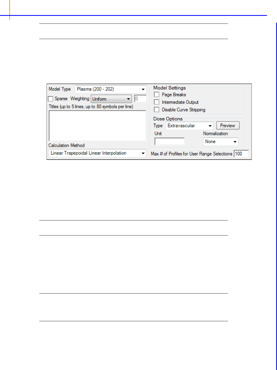
Phoenix WinNonlin

User’s Guide

126

Note: Parameter names cannot contain empty spaces. The case of each preferred parameter name is

preserved.

For more on NCA output parameters see

“NCA parameter formulas”.

Options tab

The Options tab allows users to select the NCA model and set options for the selected model.

• Use the Model Type menu to select the NCA model type (i.e., whether the input data are from

plasma, urine, or drug effect measurements). Select Plasma (200-202), Urine (210-212), or

Drug Effect (220).

• Check the Sparse checkbox to use analysis methods for sparse datasets. See

“Sparse sampling

calculation”

for more information on using sparse datasets with NCA models.

• Use the Weighting menu to select the regression that estimates Lambda Z or slopes. Select

User Defined, Uniform, 1/Y, or 1/(Y*Y).

Note: The relative proportions of the weights are important, not the weights themselves. See “Weighting”

for more on weighting schemes.

Rules for using the Weighting menu:

• If User Defined is selected then users can enter their own Observed to Power N value. The

value of N must be typed in the Weighting text field.

• Sparse data requires Uniform weighting.

• When a log-linear fit is done (Uniform weighting for Lambda Z), then the fit is implicitly using

a weighting approximately equal to 1/Yhat

Note: If 1/Y and the Linear Log Trapezoidal calculation method are selected, a user might assume that

the weighting scheme is 1/LogY, rather than 1/Y. This is not the case, however, since concentra-

tions between zero and one would have negative weights and could not be included in the analy-

sis.

• Use the Titles text box to type a title for the analysis. The title is displayed at the top of each page

in the Core Output and can include up to 5 lines of text.

• Select a method for calculating the area under the curve from the Calculation Method menu.



The chosen method applies to all AUC, AUMC, and partial area computations. All methods

NCA

127

reduce to the log trapezoidal rule, the linear trapezoidal rule, or both. The methods differ based on

when the rules are applied. See

“Partial area calculation” for descriptive equations of the calcula-

tion methods. Select from:

Linear Log Trapezoidal. This method uses the linear trapezoidal rule up to Cmax and then the

log trapezoidal rule for the remainder of the curve, to compute AUCs. Points for partial areas are

inserted using the logarithmic interpolation rule after Cmax, or after C0 for IV bolus, if C0 > Cmax.

Otherwise, the linear trapezoidal rule is used. If Cmax is not unique, then the first maximum is

used.

Linear Trapezoidal Linear Interpolation. This is the default method and recommended for Drug

Effect Data (220). It uses the linear trapezoidal rule, which is applied to each pair of consecutive

points in the dataset that have non-missing values, and sums up these areas to compute AUCs. If

a partial area is selected that has an endpoint that is not in the dataset, then the linear interpola-

tion rule is used to insert a concentration value for that endpoint.

Linear Up Log Down. The linear trapezoidal rule is used to compute AUCs any time that the con-

centration data is increasing, the logarithmic trapezoidal rule is used any time that the concentra-

tion data is decreasing. Points for partial areas are inserted using the linear interpolation rule if the

surrounding points show that concentration is increasing, and the logarithmic interpolation rule if

the concentration is decreasing.

Linear Trapezoidal Linear/Log Interpolation. This method is the same as Linear Trapezoidal

Linear Interpolation except when a partial area is selected that has an endpoint that is not in the

dataset. In that case, the logarithmic interpolation rule is used to insert points after Cmax, or after

C0 for IV bolus, if C0 > Cmax. Otherwise, the linear interpolation rule is used. If Cmax is not

unique, then the first maximum is used.

Note: The Linear Log Trapezoidal, the Linear Up Log Down, and the Linear Trapezoidal Linear/Log

Interpolation methods all apply the same exceptions in area calculation and interpolation. If a Y

value (concentration, rate, or effect) is less than or equal to zero, Phoenix defaults to the linear

trapezoidal or linear interpolation rule for that point. If adjacent Y values are equal to each other,

Phoenix defaults to the linear trapezoidal or linear interpolation rule.

Model settings

•Check the Page Breaks checkbox to include page breaks in the ASCII text output.

•Check the Intermediate Output checkbox to add to the text Core Output the values of each iter-

ation during estimation of Lambda Z and for each of the sub-areas in partial area computations.

•Check the Disable Curve Stripping checkbox to turn off Lambda Z or slope estimation for all

profiles. When this option is selected Lambda Z or slopes are not estimated, parameters that are

extrapolated to infinity are not calculated, and the Rules tab is disabled.

• Disable curve stripping for one or more individual profiles:

•Select Slopes in the Setup tab.

• Enter a start time that is greater than the last time point in a given profile and an end time

greater than the start time.

Dose options

Note: Dose Options are not available for the Drug Effect (220) model.

• Use the Type menu to select the dosing route. Dose type selections determine two things: spe-

cific model type and columns available in the Dosing panel. Select Extravascular, IV Bolus, IV

Infusion, or Dosing Defined.

Phoenix WinNonlin

User’s Guide

128

• Set the dosing unit by clicking the Units Builder - Dose […] button or typing the dosing unit into

the Unit text field. Only applicable when an internal worksheet is being used for the Dosing data.



See

“Using the Units Builder” for more details.

• Click Preview to see a preview of dose option selections in a separate window. Click OK to close

the preview window.

• Use the Normalization menu to select the appropriate factor if the dose amount is normalized by

subject body weight or body mass index. Select None, kg. g, mg, m**2, or 1.73 m**2.

If doses are in milligrams per kilogram of body weight, select mg as the dosing unit and kg as the

dose normalization.

The Normalization menu affects the output parameter units. For example, if dose volume is in

liters, selecting kg as the dose normalization changes the units to L/kg.

Dose normalization affects units for all volume and clearance parameters in NCA models, as well

as AUC/D in NCA plasma models, and Percent_Recovered in NCA urine models.

Other options

• Enter the Max # of Profiles for User Range Selections in the field (default is 100). 



If the number of profiles exceeds this value, then the user selection of slopes will be disabled and

the engine will calculate the slopes using the Best Fit method. Selecting the Slopes Selector

worksheet or Slopes worksheet will display a message notifying the user that the limit has been

exceeded and the Best Fit method will be used for all profiles.

User Defined Parameters tab

The User Defined Parameters tab allows users to include concentrations/Y values at specified times,

as well as additional NCA parameters.

•Check the Include with Final Parameters box to append the user-defined parameters (both the

computed concentrations/Ys and any additional user-defined parameters) to the Final Parame-

ters worksheets, both the pivoted and non-pivoted versions.

• Enter time or X values at which to compute the concentration or Y value.

For Plasma models, enter a value(s) in the field to have the NCA object compute the concentra-

tion (or the mean concentration, if the Sparse Sampling box in the Options tab is checked) at

that time and include the result in the output.

For Drug Effect models, enter a value(s) in the field to have the NCA object compute the Y

value at that X value and include the result in the output.



Up to 30 values can be entered as a comma-separated list. Values can also be specified by using

multiple ‘

seq’ statements with the format seq(first_time,end_time,increment). For

example,

seq(0,6,1),8,12,seq(18,36,6).

NCA

129

Note: If a concentration/drug effect value does not exist in the data set for the specified time/X value, it is

calculated following the same rules as for computing Y-values for partial area endpoints, see

“Par-

tial area calculation”.

• Click Add to define other NCA parameters to include in the output.

• Enter a name for the parameter in the Parameter column. 



The name is checked for validity as it is entered and a message is displayed in the last column of

the table if it is not valid. Since the names become column headers in the output, they must also

follow the rules for column headers: start with a letter or underscore; contain only letters, num-

bers, underscores, and ‘%’; and not contain spaces, periods, or symbols. The name cannot match

any of the following:

• default names for NCA final parameters

• preferred names for NCA final parameters

• previously defined additional NCA parameters

• names that will be generated by the Compute concentrations at times option

• the words “Dose” and “Sort”

• names of columns defined as Carry variables

• Enter an equation that defines how the parameter is to be computed in the Definition column. The

math function operators +, –, *, /, and ^ can be used in the Definition, as well as ln(x), log(x,base),

log10(x), exp(x), and sqrt(x). The parameter can be a function of the following:

• default parameter names (even if selected to be excluded from the results)

• preferred names specified on the Parameter Names setup tab (even if selected to be

excluded from the results)

• partial areas

• if an external dosing worksheet is used, the name of the column mapped to Dose and the

name of the column mapped to Tau

• if an internal dosing worksheet is used, the “Dose” and “Tau” columns

• Carry variables (names of columns mapped as Carry)

• previously defined user-defined parameter names (those that are above the current name in

the user interface)

Phoenix WinNonlin

User’s Guide

130

Note that:

• If more than one dose amount is specified for a profile, the last dose value will be used when

computing the parameter.

• If a carryalong is a time-dependent variable (that is, if the carryalong takes on different values

per profile), any user-defined parameters defined in terms of this carryalong will be unde-

fined.

• If any of the values to be used when computing the user-defined parameter are missing (for

example, an equation that uses Rsq when the Lambda Z fitting fails or was disabled), the

value of the user-defined parameter will be missing (blank) in the results.

• Any names used are case-sensitive (they must be correct in terms of uppercase and lower-

case).

• To assist with entering final parameter names in the equation, when the user starts to type a

name, a dropdown list provides a list of final parameters that match. Double-click an entry

from the list to auto-complete typing that name. The list contains only final parameters, even

though other names, such as dosing and carryalong names, can be used. The list contains all

possible final parameters in NCA, but some may not be applicable to the current selection of

model and dosing options.

• In the Units Label column enter the unit name that is to appear when the parameter values are

reported. No conversion of units is done for user-defined parameters.

• Click the red X in the row to remove that parameter.

Rules tab

The Rules tab contains optional settings that apply to the Lambda Z calculation in Plasma and Urine

models. (The Rules tab does not apply to Slope1 and Slope2 in Drug Effect models.)

Figure 17-1. Rules tab for NCA object

Lambda Z Rules for Best Fit method: These optional rules are used only in the automatic selection

of Lambda Z.

• In the Max # of points field, specify the maximum number of points that can be used in the

best-fit method for Lambda Z. If a value is specified, the NCA engine will not consider time

ranges that contain more than the specified number of points when finding the best Lambda

Z. The entered value must be at least 3.

• In the Start Time Not Before field, specify the minimum start time that can be used in the

best-fit method for Lambda Z. If a value is specified, the NCA engine will not consider time

ranges that start before this minimum start time when finding the best Lambda Z.

Lambda Z Acceptance Criteria: These optional acceptance criteria apply to both the Best Fit

method and the Time Range method. These rules are used to flag profiles (described further below)

where the Lambda Z final parameter does not meet the specified acceptance criteria.

NCA

131

• Specify the minimum value of Rsq_adjusted that indicates an acceptable fit for Lambda Z in

the Rsq_adjusted field. Value must be between 0 and 1.

• Use the pull-down menu to select whether to use AUC_%Extrap_obs or

AUC_%Extrap_pred (or, for Urine models, AURC_%Extrap_obs or AURC_%Extrap_pred)

when indicating the acceptable fit for Lambda Z. In the field, enter the maximum value to use.

Value must be between 0 and 100.

•In the Span field, specify the minimum span or number of half-lives needed for the Lambda Z

range to be acceptable. Values must be positive.

If a profile does not have an acceptable Lambda Z fit as specified by the acceptance criteria, an

output flag value of ‘Not_Accepted’ is used to flag each of the criterion that is not met by that pro-

file. In addition, a flag value of ‘Missing’ is used to flag all profiles where the parameter used for

acceptance cannot be computed. Note that all computed results for flagged profiles are still

included in the output, but the final parameters for these profiles will be marked by the flags. All

profiles that have an acceptable Lambda Z fit (i.e., meet the acceptance criterion) will have the

flag value of ‘Accepted’.

The flags appear in columns in the Final Parameters Pivoted output worksheet immediately after

the column for the parameter used for the acceptance criterion. The flag column names are ‘Flag’

appended with the parameter name used for acceptance, e.g., Flag_Rsq_adjusted, Flag_Span. If

the user wants to remove the profiles failing to meet the acceptance criteria from the output, the

Final Parameters Pivoted worksheet can be processed by the Data Wizard to delete these pro-

files, by filtering on the flag values of ‘Not_Accepted’ and excluding these rows. Note that the Flag

columns do not appear in the output when there are no flagged profiles, that is, when all profiles

meet the acceptance criterion or when the acceptance criterion is not set.

In the Final Parameters output worksheet and in the Core Output text, where the final parameter

output is stacked, the flag names and values appear below the acceptance parameter. If the

acceptance parameter is selected to not be included in the worksheet output in the “Parameters

Names” setup, the corresponding flag will also not be included in the worksheet.

See

“Data checking and pre-treatment” for a list of cases that also produce flagged output.

Plots tab

The Plots tab allows users to select individual plots to include in the output.

• Use the checkboxes to toggle the creation of graphs.

• Click Reset Existing Plots to clear all existing plot output.



Each plot in the Results tab is a single plot object. Every time a model is executed, each object

remains the same, but the values used to create the plot are updated. This way, any styles that

are applied to the plots are retained no matter how many times the model is executed. Clicking

Reset Existing Plots removes the plot objects from the Results tab, which clears any custom

changes made to the plot display.

• Use the Enable All and Disable All buttons to check or clear all checkboxes for all plots in the

list.

Phoenix WinNonlin

User’s Guide

132

Results

After an NCA object is executed, the output is displayed on the Results tab in Phoenix.

•

Worksheet output: worksheets listing input data, output parameters, as well as execution

summary.

•

Plot output: plots of observed and predicted data.

• Core Output: text version of all model settings and output, including any errors that occurred

during modeling.

• The Settings text file lists the user-specified settings in the NCA object.

Worksheet output

Worksheet output contains summary tables of the modeling data and a summary of the information in

the Core Output. The worksheets present the output in a form that can be used for reporting and fur-

ther analyses. The results worksheets are listed on the Results tab underneath Output Data.

Note: The worksheets produced depend on the analysis type and model settings.

Dosing Used: The dosing regimen specified in the Dosing panel.

Exclusions: Any excluded data points specified in the Slopes panel.

Final Parameters: Estimates of the final parameters for each level of the sort variable, including

times and areas above (“TimeHigh”), in (“TimeBetween”) and below (“TimeLow”) the therapeutic

response (AUCHigh, AUCLow, etc.). Parameter names that include “Inf” are extrapolated to infinity

using estimated Lambda Z.

Final Parameters Pivoted: The same as Final Parameters, but with one parameter per column, in

order to conveniently perform further analysis on individual parameters.

Partial Areas: Lists start and end times used to define the partial areas under the curve.

Plot Titles: The title of each graph in the output.

Slopes Settings: The settings for the user specified for the Terminal elimination phase. 

It includes the start and end time for each defined time range, excluded points, fit method used and

whether the time range was set by the System or the User.

Summary Table: The sort variables, X variable, points included in the regression for Lambda Z

(noted with *), Y variable, predicted Y for the regression, residual for the regression, area under the

curve (AUC), area under the moment curve AUMC and the weight used for the regression.

Therapeutic Response: Lists the lower and upper boundaries used to define the therapeutic

response windows.

User Defined Computed Y: List of user-entered time or X values and the concentration or Y values. 

The Type column indicates if the value was Observed or Computed by interpolation.

User Defined Parameters: List of any parameters defined by the user in the User Defined Parame-

ters tab.

User Defined Parameters Pivoted: The same as User Defined Parameters, but with one parameter

per column, in order to conveniently perform further analysis on individual parameters.

Plot output

Executing an NCA object generates an ‘Observed Y and Predicted Y vs X’ plot for each subject. Plot

output is listed underneath Plots in the Results tab.

133

Note: Hovering over a regression line in the NCA plot result (Observed Y and Predicted Y vs X plot) dis-

plays [time, conc] value pairs. However only coordinates of the predicted value at the nearest

observed time points are displayed. In other words, hovering over the regression line does not give

continuous predicted coordinates.

Phoenix WinNonlin

User’s Guide

134

NCA computation rules

Computational rules for the NCA engine are discussed in sections:

Time deviations in steady-state data

Data checking and pre-treatment

NCA computations are covered under the headings:

Lambda Z or Slope Estimation settings

Therapeutic response

Partial area calculation

Sparse sampling calculation

Drug effect calculation

Weighting

Time deviations in steady-state data

When using steady-state data, Phoenix computes AUC_TAU from dose time to dose time+tau, based

on the tau value set in the Dosing panel. However, in most studies, there are sampling time devia-

tions. For example, if dose time=0 and tau=24, the last sample might be at 23.975 or 24.083 hours. In

this instance, the program will estimate the AUC_TAU based on the estimated concentration at 24

hours, and not the concentration at the actual observation time. For steady state data, Cmax, Tmax,

Cmin and Tmin are found using observations taken at or after the dose time, but no later than dose

time+tau.

Data checking and pre-treatment

Prior to calculation of pharmacokinetic parameters, Phoenix institutes a number of data-checking and

pre-treatment procedures as follows.

• Sorting: Prior to analysis, data within each profile is sorted in ascending time order. (A profile is

identified by a unique combination of sort variable values.)

• Inserting initial time points: If a PK profile does not contain an observation at dose time, Phoe-

nix inserts a value using the following rules. (Note that, if there is no dosing time specified, the

dosing time is assumed to be zero.)

Extravascular and Infusion data: For single dose data, a concentration of zero is used; for

steady-state, the minimum observed during the dose interval (from dose time to dose time +tau)

is used.

IV Bolus data: Phoenix performs a log-linear regression of first two data points to back-extrapo-

late C0. If the regression yields a slope >= 0, or at least one of the first two y-values is zero, or if

one or both of the points is viewed as an outlier and excluded from the Lambda Z regression, then

the first observed y-value is used as an estimate for C0. If a weighting option is selected, it is

used in the regression.

Urine data: A rate value of zero is used at dose time.

Drug Effect data: An effect value equal to the user-supplied baseline is inserted at dose time

(assumed to be zero if none is supplied).

The inserted point at dose time is needed to compute the initial trapezoid from dose time to the

first observation for the AUC final parameters and to compute partial areas or therapeutic

response parameters that depend on times from the dose time to the first observation. The

inserted point is never used in Lambda Z computations.

135

Only one observation per profile at each time point is permitted. If multiple observations at the

same time point are detected, the analysis is halted with an error message. No output is gener-

ated.

• Data exclusions: NCA automatically excludes unusable data points meeting the following crite-

ria:

Missing values: For plasma models, if either the time or concentration value is missing or non-

numeric, then the associated record is excluded from the analysis. For urine models, records with

missing or non-numeric values for any of the following are excluded: collection interval start or

stop time, drug concentration, or collection volume. Also for urine models, if the collection volume

is zero, the record is excluded.

Data points preceding the dose time: If an observation time is earlier than the dosing time, then

that observation is excluded from the analysis. For urine models, the lower time point is checked.

Data points for urine models: In addition to the above rules, if the lower time is greater than or

equal to the upper time, or if the concentration or volume is negative, the data must be corrected

before NCA can run.

• Flagging data deficiencies in the Final Parameters output: After exclusion of unusable data

points as described in the prior section, profiles that result in no non-missing observations, and

profiles that result in only one non-missing observation where a valid point at dose time cannot be

inserted, have a flag called “Flag_N_Samples” in the Final Parameters output. More specifically,

these cases are:

• Profile with all missing observations (N_Samples=0) for any NCA Model Type. No Final

Parameters can be reported.

• Urine model profile with all urine volumes equal to zero. This is equivalent to no measure-

ments being taken (N_Samples=0). No Final Parameters can be reported.

• Profile with all missing observations, except one non-missing observation at dose time, for

Plasma or Drug Effect models (N=1 and a point cannot be inserted at dose time because the

one observation is already at dose time). All Final Parameters that can be defined, e.g.,

Cmax, Tmax, Cmin, Tmin, are reported. (This case does not apply to Urine models — the

midpoint of an acceptable observation would be after dose time.)

• Bolus-dosing plasma profile with all missing observations, except one non-missing observa-

tion after dose time (N=1 and a point cannot be inserted at dose time because NCA does not

back-extrapolate C0 when there is only one non-missing observation). All Final Parameters

that can be defined, e.g., Cmax, Tmax, Cmin, Tmin, are reported.

Each of these cases will have a ‘Flag_N_Samples” value in the Final Parameters output that is

‘Insufficient’. This flag allows these profiles to be filtered out of the output worksheets if desired,

using the Data Wizard.

Note: A non-bolus profile with all missing observations, except one non-missing positive observation

after dose time is not a data deficiency, because a valid point is inserted at dose time – (dose time,

0), or (dose time, Cmin) for steady state – which provides a second data point.

Lambda Z or Slope Estimation settings

This section pertains to NCA and IVIVC objects.

Phoenix will attempt to estimate the rate constant, Lambda Z, associated with the terminal elimination

phase for concentration data. If Lambda Z is estimable, parameters for concentration data will be

extrapolated to infinity. For NCA drug effect models, Phoenix estimates the two slopes at the begin-

ning and end of the data. NCA does not extrapolate beyond the observed data for drug effect models.

Phoenix WinNonlin

User’s Guide

136

Lambda Z or slope range selection

Adjusted R

1 R

–n 1–

n 2–

-------------------------------------------

–=

Phoenix will automatically determine the data points to include in Lambda Z or slope calculations as

follows. (The exception to this is if the time range to use in the calculation of Lambda Z or slopes is

not specified in an NCA object and curve stripping is not disabled, as described under “Options tab”.)

r concentration data: To estimate the best fit for Lambda Z, Phoenix repeats regressions of

the natural logarithm of the concentration values using the last three points with non-zero concen-

trations, then the last four points, last five points, etc. Points with a concentration value of zero are

not included since the logarithm cannot be taken. Points prior to Cmax, points prior to the end of

infusion, and the point at Cmax for non-bolus models, are not used in the Best Fit method (they

can only be used if the user specifically requests a time range that includes them). For each

regression, an adjusted R

is computed:

where

n is the number of data points in the regression and R

is the square of the correlation

coefficient.

Lambda Z is estimated using the regression with the largest adjusted R

and: 

– If the adjusted R

does not improve, but is within 0.0001 of the largest adjusted R

value, the

regression with the larger number of points is used. 

– Lambda Z must be calculated from at least three data points.

– The estimated slope must be negative, so that its negative Lambda Z is positive.

For sparse sampling data: For sparse data, the mean concentration at each time (plasma or

serum data) or mean rate for each interval (urine data) is used when estimating Lambda Z. Other-

wise, the method is the same as for concentration data.

For drug effect data: Phoenix will compute the best-fitting slopes at the beginning of the data

and at the end of the data using the same rules that are used for Lambda Z (best adjusted R-

square with at least three points), with the exception that linear or log regression can be used

according to the user's choice and the estimated slope can be positive or negative. If the user

specifies the range only for Slope1, then in addition to computing Slope1, the best-fitting slope for

Slope 2 will be computed at the end of the data. If the user specifies the range only for Slope2,

then the best-fitting slope for Slope 1 will be computed at the beginning of the data.

The data points included in each slope are indicated on the Summary table of the output work-

book and text for model 220. Data points for Slope1 are marked with “1” in workbook output and

footnoted using “#” in text output; data points for Slope2 are labeled “2” and footnoted using an

asterisk, “*”.

Calculation of Lambda Z

Once the time points being used in the regression have been determined either from the Best Fit

method or from the user’s specified time range, Phoenix can estimate Lambda Z by performing a

regression of the natural logarithm of the concentration values in this range of sampling times. The

estimate slope must be negative, Lambda Z is defined as the negative of the estimated slope.

Note: Using this methodology, Phoenix will almost always compute an estimate for Lambda Z. It is the

user’s responsibility to evaluate the appropriateness of the estimated value.

137

Calculation of slopes for effect data

Phoenix estimates slopes by performing a regression of the response values or their natural logarithm

depending on the user’s selection. The actual slopes are reported; they are not negated as for

Lambda Z.

Limitations of Lambda Z and slope estimation

It is not possible for Phoenix to estimate Lambda Z or slope in the following cases.

• There are only two non-missing observations and the user requested automatic range selec-

tion (Best Fit).

• The user-specified range contains fewer than two non-missing observations.

• Automatic range selection is chosen, but there are fewer than three positive concentration

values after the Cmax of the profile for non-bolus models and fewer than two for bolus models

or the slope is not negative.

• For infusion data, automatic range selection is chosen, and there are fewer than three points

at or after the infusion stop time.

• The time difference between the first and last data points in the estimation range used is

approximately < 1e –10.

In these instances, the curve fit for that subject will be omitted. The parameters that do not depend on

Lambda Z (i.e., Cmax, Tmax, AUClast, etc.) will still be reported, but the software will issue a warning

in the text output, indicating that Lambda Z was not estimable.

Therapeutic response

For non-compartmental analysis of concentration data, Phoenix computes additional parameters for

different time range computations, as listed below. The parameters included depend on whether

upper, lower, or both limits are supplied. See

“Therapeutic response windows” for additional computa-

tion details.

Time range from dose time to last observation 

Additional parameters:

TimeLow: Total time below lower limit. Included when lower or both limits are specified.

TimeBetween: Total time between lower/upper limits. Included when both limits are specified.

TimeHigh: Total time above upper limit. Included when lower or both limits are specified.

AUCLow: AUC that falls below lower limit: Included when lower or both limits are specified.

AUCBetween: AUC that falls between lower/upper limits. Included when both limits are specified.

AUCHigh: AUC that falls above upper limit. Included when lower or both limits are specified.

Time range from dose time to infinity using Lambda Z (if Lambda Z exists)

Additional parameters:

TimeInfBetween: Total time (extrapolated to infinity) between lower/upper limits. Included when

both limits are specified.

TimeInfHigh: Total time (extrapolated to infinity) above upper limit. Included when lower or both

limits are specified.

AUCInfLow: AUC (extrapolated to infinity) that falls below lower limit: Included when lower or

both limits are specified.

AUCInfBetween: AUC (extrapolated to infinity) that falls between lower/upper limits. Included

when both limits are specified.

AUCInfHigh: AUC (extrapolated to infinity) that falls above upper limit. Included when lower or

both limits are specified.

Phoenix WinNonlin

User’s Guide

138

Therapeutic response windows

For therapeutic windows, one or two boundaries for concentration values can be given, and the pro-

gram computes the time spent in each window determined by the boundaries and computes the area

under the curve contained in each window. To compute these values, for each pair of consecutive

data points, including the inserted point at dosing time if there is one, it is determined if a boundary

crossing occurred in that interval. Call the pair of time values from the dataset (

, t

i+1

) and called the

boundaries

lower

and y

upper

If no boundary crossing occurred, the difference

i+1

, t

is added to the appropriate parameter

TimeLow, TimeBetween, or TimeHigh, depending on which window the concentration values are

in. The

AUC for (t

, t

i+1

) is computed following the user’s specified AUC calculation method as

described in the section on the

“Options tab”. Call this AUC*. The parts of this AUC* are added to

the appropriate parameters

AUCLow, AUCBetween, or AUCHigh. For example, if the concentra-

tion values for this interval occur above the upper boundary, the rectangle that is under the lower

boundary is added to

AUCLow, the rectangle that is between the two boundaries is added to AUC-

Between and the piece that is left is added to AUCHigh. This is equivalent to these formulae:

AUCLow = AUCLow + y

lower

– t

)

AUCBetween = AUCBetween + (y

upper

– y

lower

)(t

– t

)

AUCHigh = AUCHigh + AUC* – y

upper

– t

)

If there was one boundary crossing, an interpolation is done to get the time value where the cross-

ing occurred; call this

t*. The interpolation is done by either the linear rule or the log rule following the

user’s AUC calculation method as described in the section on the

“Options tab”, i.e., the same rule is

used as when inserting a point for partial areas. To interpolate to get time

t* in the interval (t

, t

i+1

) at

which the concentration value is

Linear interpolation rule for time:

Log interpolation rule for time:

The AUC for (

, t*) is computed following the user’s specified AUC calculation method. The differ-

ence

t* – t

is added to the appropriate time parameter and the parts of the AUC are added to the

appropriate AUC parameters. Then the process is repeated for the interval (

t*, t

i+1

If there were two boundary crossings, an interpolation is done to get

t* as above for the first

boundary crossing, and the time and parts of AUC are added in for the interval (

, t*) as above. Then

another interpolation is done from

to t

i+1

to get the time of the second crossing t** between (t*,

i+1

), and the time and parts of AUC are added in for the interval (t*, t**). Then the times and parts of

AUC are added in for the interval (

t**, t

i+1

t* t

–

i 1+

–

----------------------

i 1+

–+=

t* t

 y

ln–ln

i 1+

ln y

ln–

-------------------------------------------

i 1+

–+=

139

The extrapolated times and areas after the last data point are now considered for the therapeutic win-

dow parameters that are extrapolated to infinity. For any of the AUC calculation methods, the AUC

rule after tlast is the log rule, unless an endpoint for the interval is negative or zero in which case the

linear rule must be used. The extrapolation rule for finding the time

t* at which the extrapolated curve

would cross the boundary concentration

is:

If the last concentration value in the dataset is zero, the zero value was used in the above compu-

tation for the last interval, but now ylast is replaced with the following if Lambda Z is estimable:

last

= exp(Lambda_z_intercept – Lambda_z(t

last

))

If ylast is in the lower window:

InfBetween and InfHigh values are the same as Between and

High values. If Lambda Z is not estimable, AUCInfLow is missing. Otherwise:

AUCInfLow = AUCLow + (y

last

/ Lambda_z)

If ylast is in the middle window for two boundaries:

InfHigh values are the same as High values.

If Lambda Z is not estimable,

InfLow and InfBetween parameters are missing. Otherwise: Use the

extrapolation rule to get

t* at the lower boundary concentration. Add time from tlast to t* into

TimeInfBetween. Compute AUC* from tlast to t*, add the rectangle that is under the lower bound-

ary into

AUCInfLow, and add the piece that is left into AUCInfBetween. Add the extrapolated area

in the lower window into

AUCInfLow. This is equivalent to:

t* = (1/Lambda_z)(Lambda_z_intercept – ln(y

lower

))

TimeInfBetween = TimeBetween + (t* – t

last

)

AUCInfBetween = AUCBetween + AUC* – y

lower

(t* – t

last

)

AUCInfLow = AUCLow + y

lower

(t* – t

last

) + y

lower

/ Lambda_z

If ylast is in the top window when only one boundary is given, the above procedure is followed

and the

InfBetween parameters become the InfHigh parameters.

If there are two boundaries and y

last

is in the top window: If Lambda Z is not estimable, all extrap-

olated parameters are missing. Otherwise, use the extrapolation rule to get

t* at the upper boundary

concentration value. Add time from tlast to

t* into TimeInfHigh. Compute AUC* for tlast to t*, add

the rectangle that is under the lower boundary into

AUCInfLow, add the rectangle that is in the mid-

dle window into

AUCInfBetween, and add the piece that is left into AUCInfHigh. Use the extrapola-

tion rule to get

t** at the lower boundary concentration value. Add time from t* to t** into

TimeInfBetween. Compute AUC** from t* to t**, add the rectangle that is under the lower bound-

ary into

AUCInfLow, and add the piece that is left into AUCInfBetween. Add the extrapolated area

in the lower window into

AUCInfLow. This is equivalent to:

t* = (1/Lambda_z)(Lambda_z_intercept – ln(y

upper

))

t** = (1/Lambda_z)(Lambda_z_intercept – ln(y

lower

))

TimeInfHigh = TimeHigh + (t* – t

last

)

TimeInfBetween = TimeBetween + (t** – t*)

Lambda_z

---------------------------





Lambda_z_intercept y

ln–=

Phoenix WinNonlin

User’s Guide

140

AUCInfHigh = AUCHigh + AUC* – y

upper

(t* – t

last

)

AUCInfBetween = AUCBetween



+ AUC* + (y

upper

– y

lower

)(t* – t

last

)

AUC** – y

lower

(t** – t*)

AUCInfLow = AUCLow + y

lower

(t* – t

last

)

lower

(t** – t*) + y

lower

/ Lambda_z

Partial area calculation

Linear trapezoidal rule

Logarithmic trapezoidal rule

where

t is (t

– t

Note: If the logarithmic trapezoidal rule fails in an interval because C

<= 0, C

<= 0, or C

, then the

linear trapezoidal rule will apply for that interval.

Linear interpolation rule (to find

C* at time t* for t

< t* < t

)

Logarithmic interpolation rule

AUC



--------------------

=

AUMC

t

 t

+

-----------------------------------------

=

AUC

t

–

------







-------------------

=

AUMC

t

 t

–

------







-----------------------------------------

 t



–

------







--------------------

–=

C* C

t* t

–

---------------

–+=

C* C



t* t

–

---------------

ln C

ln–+ln







exp=

141

Note: If the logarithmic interpolation rule fails in an interval because C

<= 0 or C

<= 0, then the linear

interpolation rule will apply for that interval.

Extrapolation (to find

C* after the last numeric observation)

Additional rules for plasma and urine models

The following additional rules apply for plasma and urine models (not model 220 for Drug Effect):

• If a start or end time falls before the first observation and after the dose time, the corresponding

value is interpolated between the first data point and

C0. C0=0 except in IV bolus models (model

201), where

C0 is the dosing time intercept estimated by Phoenix, and except for models 200 and

202 at steady state, where

C0 is the minimum value between dose time and tau.

• If a start or end time falls within the range of the data but does not coincide with an observed data

point, then a linear or logarithmic interpolation is done to estimate the corresponding

Y, according

to the AUC Calculation method selected in the NCA Options. (See

“Options tab”.) Note that loga-

rithmic interpolation is overridden by linear interpolation in the case of a non-positive endpoint.

• If a start or end time occurs after the last numeric observation (i.e., not “missing” or “BQL”) and

Lambda Z is estimable, Lambda Z is used to estimate the corresponding

Y = exp(Lambda_z_intercept – Lambda_z(t))

= [exp(

Lambda_z_intercept – Lambda_z(t

last

))]

[exp(–

Lambda_z(t – t

last

))]

= (predictedConcAtTlast)exp(–

Lambda_z(t – t

last

))

The values

Lambda_z_intercept and Lambda_z are those values found during the regression

for Lambda Z. Note that a last observation of zero will be used for linear interpolation, i.e., this rule

does not apply prior to a last observation of zero.

• If a start or end time falls after the last numeric observation and Lambda Z is not estimable, the

partial area will not be calculated.

• If both the start and end time for a partial area fall at or after the last positive observation, then the

log trapezoidal rule will be used. However, if any intervals used in computing the partial area have

non-positive endpoints or equal endpoints (for example, there is an observation of zero that is

used in computing the partial area), then the linear trapezoidal rule will override the log trapezoi-

dal rule.

• If the start time for a partial area is before the last numeric observation and the end time is after

the last numeric observation, then the log trapezoidal rule will be used for the area from the last

observation time to the end time of the partial area. However, if the last observation is non-posi-

tive or is equal to the extrapolated value for the end time of the partial area, then the linear trape-

zoidal rule will override the log trapezoidal rule.

The end time for the partial area must be greater than the start time. Both the start and end time for

the partial area must be at or after the dosing time.

Sparse sampling calculation

The NCA object provides special methods to analyze concentration data with few observations per

subject. The NCA object treats this sparse data as a special case of plasma or urine concentration

data. It first calculates the mean concentration curve of the data, by taking the mean concentration

value for each unique time value for plasma data, or the mean rate value for each unique midpoint for

Phoenix WinNonlin

User’s Guide

142

urine data. For this reason, it is recommended to use nominal time, rather than actual time, for these

analyses. The standard error of the data is also calculated for each unique time or midpoint value.

Using the mean concentration curve, the NCA object calculates all of the usual plasma or urine final

parameters listed under “NCA parameter formulas”. In addition, it uses the subje

ct information to cal-

culate standard errors that will account for any correlations in the data resulting from repeated sam-

pling of individual animals.

The NCA sparse methodology calculates PK parameters based on the mean profile for all the sub-

jects in the dataset. For batch designs, where multiple time points are measured for each subject, this

methodology only generates unbiased estimates if equal sample sizes per time point are present. If

this is not the case, then bias in the parameter estimates is introduced.

Note: In order to create unbiased estimates, the sparse sampling routines used in the NCA object

require that the dataset does not contain missing data.

For plasma data (models 200–202), the NCA object calculates the standard error for the mean con-

centration curve’s maximum value (Cmax), and for the area under the mean concentration curve from

dose time through the final observed time (AUCall). Standard error of the mean Cmax will be calcu-

lated as the sample standard deviation of the y-values at time Tmax divided by the square root of the

number of observations at Tmax, or equivalently, the sample standard error of the

y-values at Tmax.

Standard error of the mean AUC will be calculated as described in Nedelman and Jia (1998), using a

modification in Holder (2001), and will account for any correlations in the data resulting from repeated

sampling of individual animals. Specifically:

SE AUC

Var AUC

=

Since AUC is calculated by the linear trapezoidal rule as a linear combination of the mean concentra-

tion values,

where:

m=last observation time for AUCall, or time of last measurable (positive) mean concentration for

AUClast

AUC

i 0=



the sample mean at time i=

–2 i,0=

i 1+

i 1–

–2 i,1 m 1–,,=

m 1–

–2 i, m=











143

it follows that:

where:

= number of animals sampled at both times i and j 

= number of animals sampled at time i 

= sample variance of concentrations at time i 

= sample covariance between concentrations c

and c

for all animals k that are sampled at

both times

i and j

The above equations can be computed from basic statistics, and appear as equation (7.vii) in Nedel-

man and Jia (1998). When computing the sample covariances in the above, NCA uses the unbiased

sample covariance estimator, which can be found as equation (A3) in Holder (2001):

–C

–

1–1

-----

–







-----

–







----------------------------------------------------------------

k 1=



For urine models (models 210–212), the standard errors are computed for Max_Rate, the maximum

observed excretion rate, and for AURC_all, the area under the mean rate curve through the final

observed rate.

For cases where a non-zero value

C0 must be inserted at dose time t

to obtain better AUC estimates

(see “Data checking and p

re-treatment”), the AUC estimate contains an additional constant term:

C*=C0(t

– t

)/2. In other words, w

is multiplied by C0, instead of being multiplied by zero as occurs

when the point (0,0) is inserted. An added constant in AÛC will not change

Var (A ÛC) , so SE_AU-

Clast and SE_AUCall also will not change. Note that the inserted C0 is treated as a constant even

when it must be estimated from other points in the dataset, so that the variances and covariances of

those other data points are not duplicated in the

Var (A ÛC) computation.

For the case in which

=1, and r

=1 or r

=1, then s

is set to 0 (zero).

The AUCs must be calculated using one of the linear trapezoidal rules. Select a rule using the instruc-

tions listed under “Options tab”.

Drug effect calculation

NCA for drug effect data requires the following input data variables:

Dependent variable, i.e., response or effect values (continuous scale)

Independent variable, generally the time of each observation. For non-time-based data, such as

concentration-effect data, take care to interpret output parameters such as “Tmin” (independent

variable value corresponding to minimum dependent variable value) accordingly.

It also requires the following constants:

Dose time (relative to observation times), entered in the Dosing worksheet

Var AUC



------------

i 0=



-----------------------

ij



Phoenix WinNonlin

User’s Guide

144

Baseline response value, entered in the Therapeutic Response tab of the Model Properties or

pulled from a Dosing worksheet as described below

Threshold response value (optional), entered in the Therapeutic Response tab of the NCA Dia-

gram

If the user does not enter a baseline response value, the baseline is assumed to be zero, with the fol-

lowing exception. When working from a Certara Integral study that includes a Dosing worksheet, if no

baseline is provided by the user, Phoenix will use the response value at dose time as baseline, and if

the dataset does not include a response at dose time, the user will be required to supply the baseline

value.

If there is no response value at dose time, or if dose time is not given, see “Data checking and pre-

treatment” for the insertion of the point (dosetime, baseline).

Instead

of Lambda Z calculations, as computed in NCA PK models, the NCA PD model can calculate

the slope of the time-effect curve for specific data ranges in each profile. Unlike Lambda Z, these

slopes are reported as their actual value rather than their negative. See “Lambda Z or Slope Estima-

tion

settings” for more information.

ike other NCA models, the PD model can compute partial areas under the curve, but only within the

range of the data (no extrapolation is done). If a start or end time does not coincide with an observed

data point, then interpolation is done to estimate the corresponding Y, following the equations and

rules described under “Partial area calculation”.

r PD data, the default and recommended method for AUC calculation is the Linear Trapezoidal with

Linear Interpolation (set as described under “Options tab”.) Use caution with log

trapezoidal since

areas are calculated both under the curve and above the curve. If the log trapezoidal rule is appropri-

ate for the area under a curve, then it would underestimate the area over the curve. For this reason,

Phoenix uses the linear trapezoidal rule for area where the curve is below baseline when computing

AUC_Below_B, and similarly for threshold and AUC_Below_T.

Weighting

Phoenix provides flexibility in performing weighted nonlinear regression and using weighted regres-

sion. Weights are assigned using menu options or by adding weighting values to a dataset. Each

operational object in Phoenix that uses weighted values has instructions for using weighting.

There are three ways to assign weights, other than uniform weighting, through the Phoenix user inter-

face:

Weighted least squares: weight by a power of the ob

served value of Y.

Iterative reweighting: weight by a power of the pr

edicted value of Y.

Reading weights from the dataset: include weight as a column in the

dataset.

Weighted least squares

1 Y

When using weighted least squares, Phoenix weights each observation by the value of the dependent

variable raised to the power of n. That is, WEIGHT=Y

. For example, selecting this option and setting

n= –0.5 instructs Phoenix to weight the data by the square root of the reciprocal of observed Y:

If n has a negative value, and one or more of the Y values are le

ss than or equal to zero, then the cor-

responding weights are set to zero.

The application scales the weights such that the sum of the weights for each function equals the num-

ber of observations with non-zero weights. See “Scaling of weights”.

145

Iterative reweighting

1 Y



Iterative Reweighting redefines the weights for each observation to be F

, where F is the predicted

response. For example, selecting this option and setting n= –0.5 instructs Phoenix to weight the data

by the square root of reciprocal of the predicted value of Y, i.e.,

As with Weighted least squares, if N is negative, and one

or more of the predicted Y values are less

than or equal to zero, then the corresponding weights are set to zero.

Iterative reweighting differs from weighted least squares in that for weighted least squares the weights

are fixed. For iteratively re-weighted least squares the parameters change at each iteration, and

therefore the predicted values and the weights change at each iteration.

For certain types of models, iterative reweighting can be used to obtain maximum likelihood esti-

mates. For more information see the article by Jennrich and Moore (1975). Maximum likelihood esti-

mation by means of nonlinear least squares. Amer Stat Assoc Proceedings Statistical Computing

Section 57–65.

Reading weights from the dataset

It is also possible to have a variable

in the dataset that has as its values the weights to use. The

weights should be the reciprocal of the variance of the observations. As with Weighted Least

Squares, the application scales the weights such that the sum of the weights for each function equals

the number of observations with non-zero weights.

Scaling of weights

When weights are read from a dataset

or when weighted least squares is used, the weights for the

individual data values are scaled so that the sum of the weights for each function is equal to the num-

ber of data values with non-zero weights.

The scaling of the weights has no effect on the model fitting as the weights of the observations are

proportionally the same. However, scaling of the weights provides increased numerical stability.

Consider the following example:

Suppose weighted least squares with the power –2 was specified, which is the same as weighting by

1/Y*Y. The corresponding values are as shown in the third column. Each value of Y

–2

is divided by the

sum of the values in the third column, and then multiplied by the number of observations, so that:

(0.0277778/.0452254)*3=1.8426238, or 1.843 after rounding.

Note that 0.0278/0.0051 is the same proportion as 1.843/0.338.

Phoenix WinNonlin

User’s Guide

146

NCA parameter formulas

Plasma or serum data

Urine data

Sparse sampling (pre-clinical) data

Drug effect data model 220

User defined parameters

References

See also “NCA” and, for additional reading, see “References”.

Plasma or serum data

Data structure: NCA for blood concentration data requires the following input data:

• Time of each sample

• Plasma or serum concentrations

Output: Models 200–202 estimate the parameters in the following lists.

Plasma parameters that do not require Lambda Z estimation

Plasma parameters that are estimated when Lambda Z is estimated

Plasma parameters that are estimated when at steady-state

Plasma parameters that do not require Lambda Z estimation

Dosing time: Available as ‘Time’ in the Dosing Used results. Time of last administered dose. It is

assumed to be zero unless otherwise specified. This parameter is used mainly with steady-state data,

where time may be coded as the time elapsed since the first dose, or the elapsed time since the time

of the first dose.

N_Samples: This parameter reports the number of non-missing observations used in the analysis of

the profile (time is at or after dosing time, the observation is numeric, and the volume is positive for

urine models). It does not count points inserted by engine, e.g., inserted at dosing time.

Dose: Amount of last administered dose. This is assumed to be zero if not specified.

No_points_Lambda_z: Number of points used in computing Lambda Z. If Lambda Z is not estima-

ble, zero.

Tlag: Time of observation prior to the first observation with a measurable (non-zero) concentration.

For plasma models, Tlag is only computed when the dosing type is extravascular.

Tmax: Time of maximum observed concentration. For non-steady-state data, the entire curve is con-

sidered. If the maximum observed concentration is not unique, then the first maximum is used.

Cmax: Maximum observed concentration, occurring at time Tmax, as defined above.

Cmax_D: =

Cmax/Dose

C0: Initial concentration. Given only for IV Bolus dosing. It is equal to the first observed concentration

value if that value occurs at the dose time. Otherwise, it is estimated by back-extrapolating (see

AUC_%Back_Ext below).

Tlast: Time of last measurable (positive) observed concentration.

Clast: Observed concentration corresponding to Tlast.

AUClast: Area under the curve from the time of dosing to the time of the last measurable (positive)

concentration (Tlast).

147

AUClast_D: = AUClast/Dose

AUCall: Area under the curve from the time of dosing to the time of the last observation. If the last

concentration is positive, AUClast=AUCall. Otherwise, AUCall will not be equal to AUClast, as it

includes the additional area from the last measurable (positive) concentration down to zero or nega-

tive observations.

AUMClast: Area under the moment curve from the time of dosing to the last measurable (positive)

concentration.

MRTlast: Mean residence time from the time of dosing to the time of the last measurable concentra-

tion.

For non-infusion models: =

AUMClast/AUClast



For infusion models: = (AUMClast/AUClast) – (Tinf/2)

where

Tinf is the length of infusion.

Plasma parameters that are estimated when Lambda Z is estimated

The following list includes several parameters that are extrapolated to infinity. These parameters are

calculated two ways: based on the last observed concentration (indicated by “_obs” appended to the

parameter name), or based on the last predicted concentration (indicated by “_pred” appended to the

parameter name), where the predicted value is based on the linear regression performed to estimate

Lambda Z.

Rsq: Goodness of fit statistic for the terminal elimination phase.

Rsq_adjusted: Goodness of fit statistic for the terminal elimination phase, adjusted for the number of

points used in the estimation of Lambda Z.

Corr_XY: Correlation between time (X) and log concentration (Y) for the points used in the estimation

of Lambda Z.

Lambda_z: First-order rate constant associated with the terminal (log-linear) portion of the curve.

Estimated by linear regression of time vs. log concentration.

Lambda_z_intercept: Intercept on log scale estimated via linear regression of time vs. log concentra-

tion.

Lambda_z_lower: Lower limit on time for values to be included in the calculation of Lambda Z.

Lambda_z_upper: Upper limit on time for values to be included in the calculation of Lambda Z.

HL_Lambda_z: Terminal half-life: = ln(2)/



Span: = (

Lambda_z_upper – Lambda_z_lower)/HL_Lambda_z

Clast_pred: Predicted concentration at

Tlast:

exp(Lambda_z_intercept – Lambda_z*Tlast)

AUCINF(_obs, _pred): AUC from time of dosing extrapolated to infinity, based on the last observed

concentration (_obs) or last predicted concentration (_pred).

AUClast + (Clast/Lambda_z)

AUCINF_D(_obs, _pred): =

AUCINF/Dose

AUC_%Extrap(_obs, _pred): Percentage of AUCINF(_obs, _pred) due to extrapolation from Tlast to

infinity:

= 100[(

AUCINF– AUClast)/AUCINF]

Phoenix WinNonlin

User’s Guide

148

AUC_%Back_Ext(_obs, _pred): Computed for IV Bolus models. Percentage of AUCINF that was

due to back extrapolation to estimate C0 when the first measured concentration is not at dosing time.

Vz(_obs, _pred), Vz_F(_obs, _pred)

: Volume of distribution based on the terminal phase.

For non-steady-state data: =

Dose/[Lambda_z(AUCINF)]

Cl(_obs, _pred), Cl_F(_obs, _pred)

: Total body clearance for extravascular administration.

Dose/AUCINF

AUMCINF(_obs, _pred): Area under the first moment curve (AUMC) extrapolated to infinity, based

on the last observed concentration (obs) or the last predicted concentration (pred).

AUMC_%Extrap(_obs, _pred): Percent of AUMCINF(_obs, _pred) that is extrapolated.

= 100[(

AUMCINF – AUMClast)/AUMCINF]

MRTINF(_obs, _pred): Mean residence time (MRT) extrapolated to infinity. For non-steady-state

data:

For non-infusion models: =

AUMCINF/AUCINF 

For infusion models: = (

AUMCINF/AUCINF) – (Tinf/2)

where

Tinf is the length of infusion. 

(Note that, for extravascular dosing (oral model 200), MRTINF includes Mean Input Time as well

as time in systemic circulation.)

Vss(_obs, _pred): For non-steady-state data: An estimate of the volume of distribution at steady-

state based on the last observed (obs) or last predicted (pred) concentration.

= (MRTINF)(CL)

Computed for IV Bolus and Infusion dosing only. Not computed for extravascular dosing (oral model

200), as MRTINF for oral models includes Mean Input Time as well as time in systemic circulation and

therefore is not appropriate to use in calculating Vss.

For extravascular models (model 200), the fraction of dose absorbed cannot be estimated; therefore

Volume and Clearance for these models are actually Volume/F or Clearance/F where F is the fraction

of dose absorbed.

Plasma parameters that are estimated when at steady-state

Tau: Available in the Dosing Used results worksheet for steady-state data. The (assumed equal) dos-

ing interval for steady-state data.

Tmax: Time of maximum observed concentration. For steady-state data, based on observations col-

lected during the dosing interval, that is, at or after the dosing time, but no later than the dosing time

plus Tau, where Tau is the dosing interval. If the maximum observed concentration is not unique, then

the first maximum is used.

Cmax: Maximum observed concentration, occurring at time Tmax, as defined above.

Tmin: Time of minimum observed concentration. For steady-state data, based on observations col-

lected during the dosing interval (i.e., after the dosing time, but no later than dosing time plus Tau,

where Tau is the dosing interval). If the minimum observed concentration is not unique, then the first

minimum is used.

AUMClast

tlast Clast

Lambda_z

------------------------------

Clast

Lambda_z

------------------------------

149

Cmin: Minimum observed concentration occurring at time Tmin as defined above.

Note: Regulatory agencies differ on the definition of Cmin: some agencies define Cmin the same

as Ctau is defined below. Both Cmin and Ctau are included in the output so that users can use the

correct parameter for their situation.

Ctau: Concentration at dosing time plus Tau. Observed concentration if the value exists in the input

data; otherwise, the predicted concentration value. Predicted concentrations are calculated following

the same rules as for computing inserting missing endpoints needed for partial areas, see

“Partial

area calculation”.

Cavg: Average concentration, computed = AUC_TAU/Tau

Swing: = (Cmax – Cmin)/Cmin

Swing_Tau: = (Cmax – Ctau)/Ctau

Fluctuation%: = 100[(Cmax – Cmin)/Cavg] where Cmin and Cmax were obtained between dos-

ing time and dosing time plus Tau.

Fluctuation%_Tau: = 100[(Cmax – Ctau)/Cavg]

CLss, CLss_F

: An estimate of the total body clearance, computed for IV Bolus and Infusion dosing

only.

MRTINF(_obs, _pred): Mean residence time (MRT) extrapolated to infinity based on AUCINF(_obs,

_pred).

For non-infusion: 

For infusion: 

where TI represents infusion duration. (Note that, for oral model 200, MRTINF includes Mean

Input Time as well as time in systemic circulation.)

Vz, Vz_F

: =

Vss(_obs, _pred): An estimate of the volume of distribution at steady-state based on the last

observed (obs) or last predicted (pred) concentration. Computed for IV Bolus and infusion dosing

only.

MRTINF(CLss)

Not computed for extravascular dosing (oral model 200), as MRTINF for oral models includes Mean

Input Time as well as time in systemic circulation and therefore is not appropriate to use in calculating

Vss.

Dose

AUC



-----------------

AUMC



 AUCINF AUC



–+

AUC



-----------------------------------------------------------------------------------

AUMC



 AUCINF AUC



–+

AUC



-----------------------------------------------------------------------------------

-----

–

Dose



AUC





---------------------------

Phoenix WinNonlin

User’s Guide

150

Accumulation Index: =

AUC_TAU: The partial area from dosing time to dosing time plus Tau. See

“Partial area calculation”

for information on how it is computed.

AUC_TAU_D: =

AUC_TAU/Dose

AUC_TAU_%Extrap: Percentage of AUC_TAU that is due to extrapolation from Tlast to dosing time

plus Tau.

= 

AUMC_TAU: Area under the first moment curve from dosing time to dosing time plus Tau. See

“Par-

tial area calculation”

for information on how it is computed.

AUClower_upper: (Optional) User-requested area(s) under the curve from time “lower” to “upper”.

For extravascular models (model 200), the fraction of dose absorbed cannot be estimated; therefore

Volume and Clearance for these models are actually Volume/F or Clearance/F where F is the fraction

of dose absorbed.

Urine data

Data structure: NCA for urine data requires the following input data:

Starting and ending time of each urine collection interval

Urine concentrations

Urine volumes

From this data, models 210–212 compute the following for the analysis:

Midpoint of each collection interval=(Starting time+Ending time)/2

Excretion rate for each interval (amount eliminated per unit of time)=(Concentration*Volume)/

(Ending time-Starting time)

Output: Models 210–212 estimate the following parameters.

The worksheet will include the Sort(s), Carry(ies), parameter names, units, and computed values. A

User Defined Parameters Pivoted worksheet will include the pivoted form of the User Defined Param-

eters worksheet.

Urine parameters that do not depend on Lambda Z

Dosing time: Available as ‘Time’ in the Dosing Used results. Time of last administered dose. It is

assumed to be zero unless otherwise specified. This parameter is used mainly with steady-state data,

where time may be coded as the time elapsed since the first dose, or the elapsed time since the time

of the first dose.

Dose: Amount of last administered dose. This is assumed to be zero if not specified.

N_Samples: Number of non-missing observations in the analysis. Does not include missing or non-

numeric observations, observations before dosing time, or urine observations where volume is zero.

Does not include the point at dosing time if it was not observed but was inserted by the engine.

1 e

Lambda_z–

–

---------------------------------------------

100

AUC_TAU AUClast–

AUC_TAU

---------------------------------------------------------

if Dosing_Time  Tlast+,

0 if Dosing_Time  Tlast+,

151

No_points_lambda_z: Number of points used in the computation of Lambda Z. If Lambda Z cannot

be estimated, this is set to zero.

Tlag: Midpoint of the collection interval prior to the first collection interval with measurable (non-zero)

rate. Computed for all urine models.

Tmax_Rate: Midpoint of the collection interval associated with the maximum observed excretion rate. 

If the maximum observed excretion rate is not unique, then the first maximum is used.

Max_Rate: Maximum observed excretion rate, at time Tmax_Rate as defined above.

Mid_Pt_last: Midpoint of collection interval associated with last measurable (positive) observed

excretion rate.

Rate_last: Last observed measurable (positive) rate at time Mid_Pt_last.

AURC_last: Area under the urinary excretion rate curve from time of dosing to Mid_Pt_last.

AURC_last_D: =

AURC_last/Dose

Vol_UR: Sum of Urine Volumes (urine)

Amount_Recovered: Cumulative amount eliminated.

Percent_Recovered: = 100(

Amount_Recovered/Dose)

AURC_all: Area under the urinary excretion rate curve from the time of dosing to the midpoint of the

interval with the last rate. If the last rate is positive, AURC_last=AURC_all.

Urine parameters that are estimated when Lambda Z is estimated

The following list includes some parameters that are extrapolated to infinity. These parameters are

calculated two ways: based on the last observed excretion rate: Rate_last (indicated by “_obs”

appended to the parameter name), or based on the last predicted excretion rate: Rate_last_pred

(indicated by “_pred” appended to the parameter name), where the predicted value is based on the

linear regression performed to estimate Lambda Z.

Rsq: Goodness of fit statistic for the terminal elimination phase.

Rsq_adjusted: Goodness of fit statistic for the terminal elimination phase, adjusted for the number of

points used in the estimation of Lambda Z.

Corr_XY: Correlation between midpoints and log excretion rates for the points used in the estimation

of Lambda Z.

Lambda_z: First-order rate constant associated with the terminal (log-linear) portion of the curve.

This is estimated via linear regression of midpoints vs. log excretion rates.

Lambda_z_intercept: Intercept on log scale estimated via linear regression of midpoints vs. log

excretion rates.

Lambda_z_lower: Lower limit on midpoint for values to be included in Lambda Z estimation.

Lambda_z_upper: Upper limit on midpoint for values to be included in Lambda Z estimation.

HL_Lambda_z: Terminal half-life=ln(2)/

Lambda Z

Span: = (

Lambda_z_upper – Lambda_z_lower)/HL_Lambda_z

Rate_last_pred: Predicted rate at Mid_Pt_last.

AURC_INF(_obs, _pred): Area under the urinary excretion rate curve extrapolated to infinity, based

on the last observed excretion rate (_obs) or the last predicted rate (_pred), i.e., the excretion rate at

Concentration_Volume



Phoenix WinNonlin

User’s Guide

152

the final midpoint estimated using the linear regression for Lambda Z. Note that AURC_INF is theoret-

ically equal to Amount_Recovered, but will differ due to experimental error.

AURC_%Extrap(_obs, _pred): Percent of AURC_INF(_obs, _pred) that is extrapolated.

Sparse sampling (pre-clinical) data

When an NCA model is loaded with the Sparse Sampling option (see “Options tab”), the data are

treated as a special case of plasma or urine concentration data. The NCA engine computes the mean

concentration or rate at each unique time value or interval. Using the mean concentration curve

across subjects, it estimates the same parameters normally calculated for plasma or urine data, plus

those listed below. See

“Sparse sampling calculation” for additional details of NCA computations with

sparse data.

Note: The names of some of the output worksheets change when the data is sparse: Final Parameters

becomes Mean Curve Final Parameters, and Summary Table becomes Mean Curve Summary

Table.

Plasma or serum concentration parameters

Sparse sampling methods for plasma data (models 200–202) compute the following parameters in

addition to those listed in

“Plasma or serum data”.

SE_Cmax: Standard error of data at Tmax (time of maximum mean concentration).

SE_AUClast: It is the standard error of the area under the mean concentration curve from dose time

to Tlast, where Tlast is the time of last measurable (positive) mean concentration.

SE_AUCall: Standard error of the area under the mean concentration curve from dose time to the

final observation time.

Note: SE_AUClast and SE_AUCall provide a measurement of the uncertainty for AUClast and AUCall,

respectively, and are usually the same. Differences between these parameter values will only be

observed if some of the measurements were flagged as BQL (below the quantitation limit).

Note: With Sparse Sampling, since SE for AUC computations depend on AUC being a linear combina-

tion of the mean concentrations, SE_AUClast and SE_AUCall are not included in the output when

the output when log trapezoidal rules are specified as the method for computing AUC.

Urine excretion rate parameters

Sparse sampling methods for urine data (models 210–212) compute the following parameters in addi-

tion to those listed under

“Urine data”.

SE_Max_Rate: Standard error of the data at the time of maximum mean rate.

SE_AURC_last: Standard error of the area under the mean urinary excretion rate curve from dose

time through the last interval that has a measurable (positive) mean rate.

SE_AURC_all: Standard error of the area under the mean urinary excretion rate curve from dose

time through the final interval.

153

Individuals by time

This sheet includes the individual subject data, along with N (number of non-missing observations),

the mean and standard error for each unique time value (plasma data) or unique midpoint value (urine

data).

References

Holder (2001). Comments on Nedelman and Jia's extension of Satterthwaite's approximation applied

to pharmacokinetics. J Biopharm Stat 11(1-2):75–9.

Nedelman, Gibiansky and Lau (1995). Applying Bailer's method for AUC intervals to sparse sampling.

Pharm Res 12:124–8.

Nedelman and Jia (1998). An extension of Satterthwaite's approximation applied to pharmacokinet-

ics. J Biopharm Stat 8(2):317–28.

Yeh (1990). Estimation and Significant Tests of Area Under the Curve Derived from Incomplete Blood

Sampling. ASA Proceedings of the Biopharmaceutical Section 74–81.

Drug effect data model 220

Figure 20-1. Illustration of a time-effect curve with AUCs highlighted

Output parameter names use the following conventions:

B is the baseline effect value (discussed above).

T is the user-supplied threshold effect value.

“Above” means towards increasing Y values, even for inhibitory effects.

Estimated parameters for model 220

N_Samples: This parameter reports the number of non-missing observations used in the analysis of

the profile (time is at or after dosing time, the observation is numeric, and the volume is positive for

urine models). It does not count points inserted by engine, e.g., inserted at dosing time.

Slope1 (or 2): Slope of the first (or second) segment of the curve. See

“Lambda Z or Slope Estimation

settings”

Rsq_Slope1 (or 2): Goodness of fit statistic for slope 1 or 2.

Rsq_adj_Slope1 (or 2): Goodness of fit statistic for slope 1 or 2, adjusted for the number of points

used in the estimation.

Phoenix WinNonlin

User’s Guide

154

Corr_XY_Slope1 (or 2): Correlation between time (X) and effect (or log effect, for log regression) (Y)

for the points used in the slope estimation.

No_points_Slope1 (or 2): The number of data points included in calculation of slope 1 or 2.

Slope1_lower or Slope2_lower: Lower limit on Time for values to be included in the slope calcula-

tion.

Slope1_upper or Slope2_upper: Upper limit on Time for values to be included in the slope calcula-

tion.

Tmin: Time of minimum observed response value (Rmin).

Rmin: Minimum observed response value.

Tmax: Time of maximum observed response value (Rmax).

Rmax: Maximum observed response value.

Baseline: Baseline response (Y) value supplied by the user, (assumed to be zero if none is supplied)

or, for Certara Integral studies with no user-supplied baseline value, effect value at dose time.

AUC_Above_B: Area under the response curve that is above the baseline (dark gray areas in the

above diagram).

AUC_Below_B: Area that is below the baseline and above the response curve (combined blue and

pink areas in the above diagram).

AUC_Net_B: =

AUC_Above_B – AUC_Below_B. This is likely to be a negative value for inhibitory

effects.

Time_Above_B: Total time that Response is greater than or equal to Baseline.

Time_Below_B: Total time that Response is less than Baseline.

Time_%Below_B: = 100*

Time_Below_B/(Tfinal – Tdose), where Tfinal is the final observation

time and

Tdose is dosing time.

When a threshold value is provided, model 220 also computes the following.

Threshold: Threshold value used.

AUC_Above_T: Area under the response curve that is above the threshold value (combined light and

dark gray areas in the above diagram).

AUC_Below_T: Area that is below the threshold and above the response curve (pink area in the

above diagram).

AUC_Net_T: =

AUC_Above_T – AUC_Below_T

Time_Above_T: Total time that Response >= Threshold.

Time_Below_T: Total time that Response < Threshold.

Time_%Below_T: = 100*

Time_Below_T/(Tlast – Tdose) 

where Tlast is the final observation time and Tdose is dosing time.

Tonset: Time that the response first crosses the threshold coming from the direction of the baseline

value, as shown in the above diagram.

Tonset=Tdose if the first response value is across the thresh-

old, relative to baseline. The time will be interpolated using the calculation method selected in the

model options. (See

“Options tab”.)

Toffset: Time greater than Tonset at which the curve first crosses back to the baseline side of thresh-

old, as shown in the diagram above.

155

Diff_Toffset_Tonset: = Toffset – Tonset

Time_Between_BT: Total time spent between baseline and threshold (sum of length of green arrows

in diagram).

AUClower_upper: (Optional) user-requested area(s) under the curve from time “lower” to time

“upper”.

Use caution in interpreting Tonset and Toffset for noisy data if Baseline and Threshold are close

together.

User defined parameters

Any user defined parameters will be computed and reported in the User Defined Parameters and

User Defined Parameters Pivoted worksheets. The worksheets include entries for Sort, Carry, param-

eter name, unit, and estimated value. A User Defined Parameters Pivoted worksheet will include the

pivoted form of the User Defined Parameters worksheet.

C<time value>: For Plasma models with user-defined times only, one column per requested time

value. (For plasma models, a computed concentration at time zero will be reported as the parameter

C0_0, since C0 is already used for the initial concentration measurement.)

Y<x-value>: For Drug Effect models with user-defined x-values only, one column per requested x-

value.

<user-defined name>: Parameter defined using the User Defined Parameters tab.

References

Holder (2001). “Comments on Nedelman and Jia's extension of Satterthwaite's approximation applied

to pharmacokinetics.” J Biopharm Stat 11(1–2):75–9.

Nedelman and Jia (1998). “An extension of Satterthwaite's approximation applied to pharmacokinet-

ics.” J Biopharm Stat 8(2):317–28.

Phoenix WinNonlin

User’s Guide

156

NCA examples

This section presents several examples of the NCA operational object usage within Phoenix. Knowl-

edge of how to do basic tasks using the Phoenix interface, such as creating a project and importing

data, is assumed.

The examples include:

Analysis of three profiles using NCA

Exclusion and partial area NCA example

Sparse sampling NCA example

Urine study NCA example

Drug effect NCA example

Multiple profile analysis using NCA

Analysis of three profiles using NCA

Suppose a researcher has obtained time and concentration data following oral administration of a test

compound to three subjects, and wants to perform noncompartmental analysis and summarize the

results.

The completed project (

NCA.phxproj) is available for reference in …\Examples\WinNonlin.

Set up the project and data for the three profiles

Create a new project named NCA.

2. Import the file …\Examples\WinNonlin\Supporting files\Bguide1 single

dose and steady state.dat

Note: Units must be added to the time and concentration columns before the dataset can be used in a

noncompartmental analysis.

3. With Bguide1 single dose and steady state selected in the Data folder, go to the Columns tab

(lower part of the Phoenix window) and select the Time column header in the Columns box.

4. Clear the Unit field and type hr.

5. Select the Conc column header in the Columns box.

6. Clear the Unit field and type ng/mL.

Or 

Click the Units Builder button and use the Units Builder dialog tools

Note: Units added to ASCII datasets can be preserved if the datasets are saved in .dat or .csv file

format. Phoenix adds the units to a row below the column headers. To import a

.dat or .csv file

with units, select the Has units row option in the File Import Wizard dialog.

Set up the NCA object for analysis of the three profiles

Noncompartmental analysis for extravascular dosing is available as Model 200 in the Phoenix model

library. Phoenix displays the model type (Plasma, Urine, or Drug Effect) in the Options tab of an NCA

object.

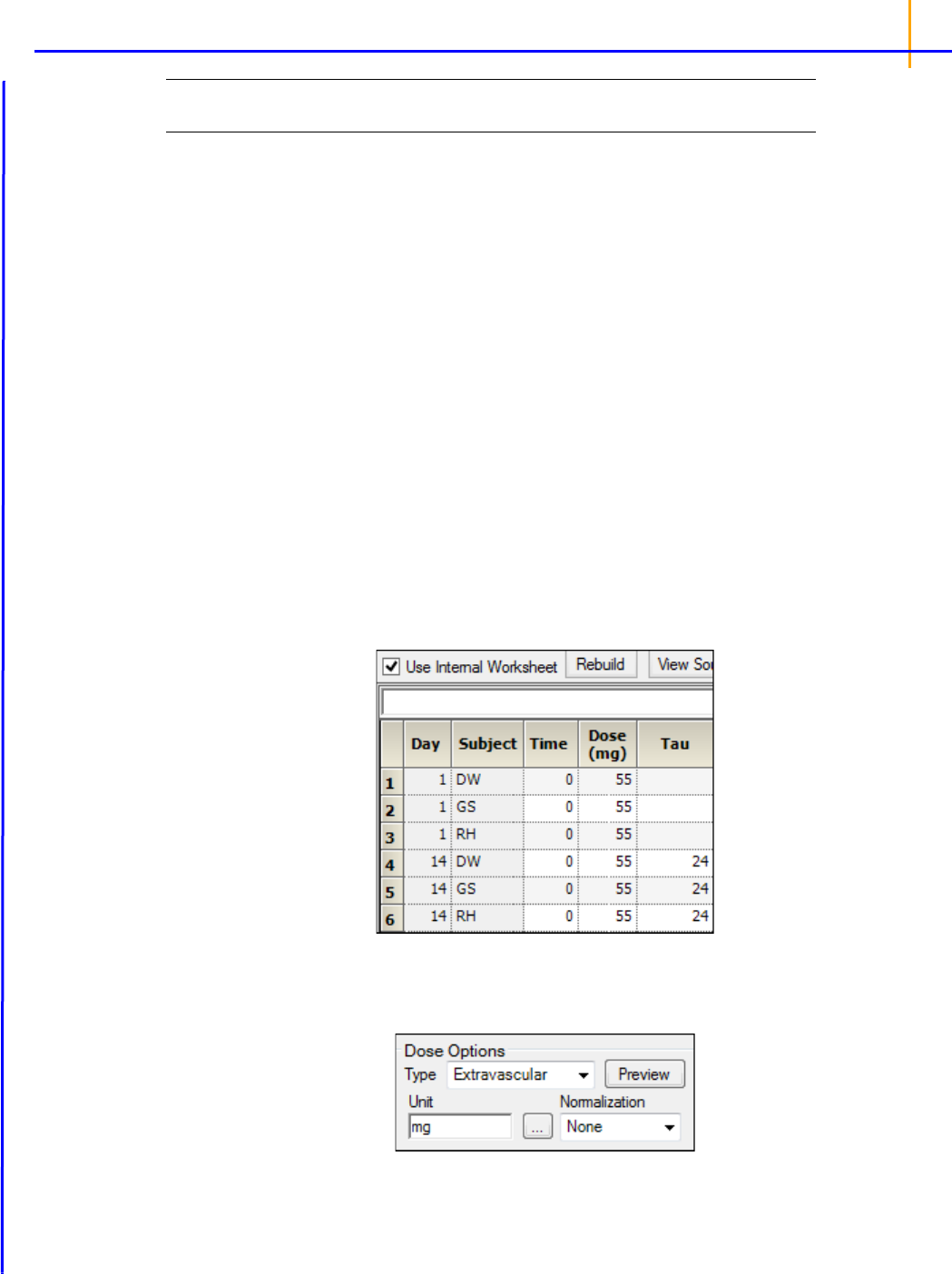
157

Note: The exact model used is determined by the dose type. Extravascular Input uses Model 200, IV-

Bolus Input uses Model 201, and Constant Infusion uses Model 202.

1. Select Workflow in the Object Browser and then select Insert > NonCompartmental Analysis >

NCA.

2. Drag the Bguide1 single dose and steady state worksheet from the Data folder to the NCA

object’s Main Mappings panel.

3. Map the data types as follows:

Day to the Sort context (make sure to map Day first) 

Subject to the Sort context 

Time mapped to the Time context 

Conc to the Concentration context

Prepare the dosing information from the profiles

Select Dosing in the NCA object's Setup list.

2. In the Dosing panel, select the Use Internal Worksheet checkbox.

3. Click OK in the Select sorts dialog to accept the default sort variables.

4. For each row:

In the Time column, enter

0.

In the Dose column, enter

55. 

In the Tau column, enter

24 for the three Day 14 rows (rows 4, 5, and 6).

5. In the Dose Options area of the Options tab, type mg in the Unit field and press the Enter key.

The units are immediately added to the column header.

6. Extravascular is selected by default in the Type menu. Do not change this setting.

Phoenix WinNonlin

User’s Guide

158

Set up the terminal elimination phase for the analysis

Phoenix attempts to estimate the rate constant Lambda Z, associated with the terminal elimination

phase. Although Phoenix is capable of selecting the times to be used in the estimation of Lambda Z,

this example provides Phoenix with the time range.

Specify the times to be included.

1. Select Slopes in the Setup list.

2. For each row:

In the Start Time column, type

8.

In the End Time column, type

24.

Do not type any values into the Exclusions column.

3. Select Slopes Selector in the Setup list. 



The Time Range is selected in the Lambda Z Calculation Method menu. The Start and End

times have been specified for each subject. A line is displayed on each graph that shows the

Lambda Z time range.



In this example, no points are excluded from the specified Lambda Z time range. The example

“Exclusion and partial area NCA example” demonstrates Lambda Z exclusions.

Specify therapeutic response options

The next step is to define a target concentration range to enable calculation of the time and area

located above, below, and within that range.

Note: See “Exclusion and partial area NCA example” for an NCA example that includes computation of

partial areas under the curve.

1. Select Therapeutic Response in the Setup list.

2. Select the Use Internal Worksheet checkbox.

3. Click OK in the sorts dialog to accept the default sort variables.

4. For each row:

Type

2 in the Lower column.

Type

4 in the Upper column.

Set preferred units for the analysis

The next step in setting options is to specify preferred output units. The independent variable, depen-

dent variable, and dosing regimen must have units before preferred output units can be set.

1. Select Units in the Setup list.



The Units worksheet lists both the Default units and the Preferred units for each parameter. The

new preferred volume unit needs to be set to L (liter).

2. Select the cell in the Preferred column for Volume (Vz, Vz/F, Vss).

3. Type L and press ENTER.

159

Specify NCA model options for the analysis

Four methods are available for computing the area under the curve. The default method is the linear

trapezoidal rule with linear interpolation. This example uses the Linear Log Trapezoidal method: lin-

ear trapezoidal rule up to Tmax, and log trapezoidal rule for the remainder of the curve.

Use the Options tab to specify settings for the NCA model options. The Options tab is located under-

neath the Setup tab.

1. Select Linear Log Trapezoidal in the Calculation Method menu.

2. In the Titles field type Example of Noncompartmental Analysis.

Set an acceptance criteria rule

Acceptance criteria for Lambda Z, which are applicable to both the Best Fit method and the Time

Range method, can be specified on the Rules tab. These rules are used to flag profiles where the

Lambda_z final parameter does not meet the specified acceptance criteria.

1. Select the Rules tab.

2. In the Rsq_adjusted field, type 0.97 to flag any profile with an Rsq_adjusted value greater than

or equal to this value.

Profiles that break the rule are flagged in the output and can be quickly filtered out of the results. The

process will be illustrated later in this example.

Execute and view the results of the analysis

At this point, all of the necessary commands have been specified.

1. Click (Execute icon) to execute the object.

2. In the Results tab, select Final Parameters in the list.



Subject DW’s concentrations were within the theoretical therapeutic range for just over 13.8 hours,

as reflected in the parameter TimeBetween.

3. In the Results tab, select Observed Y and Predicted Y vs X in the list.



The NCA object’s plot output includes Observed Y and Predicted Y vs X graphs for each subject

(switch between the plots using the tabs below the graph).

Phoenix WinNonlin

User’s Guide

160

4. In the Results tab, select Core output in the list.



The NCA object’s Core Output text file contains user settings, a brief summary table, and final

parameters output for each subject.

Figure 21-1. Settings portion of the Core Output

Filter out flagged profiles

In the Results tab, select Final Parameters Pivoted in the list.

161

Figure 21-2. Part of the Final Parameters Pivoted worksheet

For this example, a rule was set for the value of Rsq_adjusted (see “Set an acceptance criteria rule”).

The output indicates that the profile for DW broke this rule with a value of ‘Accepted’ in the Flag_R-

sq_adjusted column.

To remove any profiles failing to meet acceptance criteria from the output, the Final Parameters Piv-

oted worksheet can be processed by the Data Wizard to delete these profiles. The worksheet is fil-

tered on the flag values of 'Not Accepted' and identified rows are then excluded.

Note: The NCA.phxproj file does not include processing by the Data Wizard, but the information is

included here as a reference.

a) Insert a Data Wizard object.

b) In the Options tab, set Action to Filter and click Add.

c) Click the Select Source icon in the Mappings panel and select the NCA Final Parameter Piv-

oted worksheet.

d) In the Options tab, click the Add button to the right of the Specify Filter field.

e) In the Filter Specification dialog, define the filter to Exclude rows that have a value of Not

Accepted in the Flag_Rsq_adjusted column (or other “Flag_” column on which you want to filter

profiles).

Once the filter is defined, execute the Data Wizard object.

Summarize the analysis output with statistics

At this point, it is convenient to summarize the results of the noncompartmental analysis using a

Descriptive Statistics object. This example summarizes parameter estimates across subjects.

1. Select Workflow in the Object Browser and then select Insert > Computation Tools > Descrip-

tive Statistics.

2. In the Descriptive Statistic’s Main Mappings panel click the Select Source icon.

3. Under the NCA node, select the Final Parameters worksheet and click OK.

4. In the Main Mappings panel, map the data types to the following contexts:

Map Day to the Sort context (make sure to map Day first).

Leave Subject mapped to None.

Map Parameter to the Sort context.

Leave Units mapped to None.

Map Estimate to the Summary context.

Note: Mapping Day and Parameter to Sort computes statistics on the parameter estimates for each day

and mapping Estimate to Summary computes one statistic per parameter per day.

Phoenix WinNonlin

User’s Guide

162

5. In the Options tab, check the Confidence Intervals and Number of SD Statistics checkboxes,

but do not change the default values for these two items.

6. Execute the object.

The three subjects spent an average of 13.6 hours within the therapeutic concentration range on Day

1, as shown by the parameter TimeBetween.

Use ratios to compare data

The Ratios and Differences object can be used to quickly setup ratios and/or differences between

parameter values in order to compare data. A description of the object can be found in

“Ratios and

Differences”

1. In the Object Browser, click the NCA object.

2. In the Results list, right-click Final Parameters Pivoted and select Send To > Computation

Tools > Ratios and Differences.

3. In the Main Mappings panel of the Ratios and Differences object, map the data types to the follow-

ing contexts:

Map Day to the Filter context.

Map Subject to the Sort context.

Map the rest of the data types to the Carry context by first mapping N_Samples to Carry and then

drag the corner of the selected cell all the way to the bottom of the grid. It may take a few seconds.

4. In the Options tab, set up two ratios as shown in the following image. Use the Add button to add

the second row of options to the table.

5. Execute the object.

6. In the Results tab, select Ratios Differences and compare the ratios for each subject.

This concludes the multiple profile example.

163

Exclusion and partial area NCA example

This example demonstrates the exclusion of points in the terminal elimination phase and computation

of partial area under the curve in the Phoenix NCA object. The time-concentration data is for a single

subject and the data is provided in

NCA2.csv, which is located in the Phoenix examples directory.

Noncompartmental analysis for extravascular dosing is available as model 200 in Phoenix’s noncom-

partmental analysis object. Phoenix always displays the model type in the NCA object’s Options tab.

Note: The exact model used is determined by the dose type. Extravascular Input uses Model 200, IV-

Bolus Input uses Model 201, and Constant Infusion uses Model 202.

The completed project (

NCA_PartialAreas.phxproj) is available for reference in …\Exam-

ples\WinNonlin

Set up the NCA object

Create a project called NCA_PartialAreas.

2. Import the file …\Examples\WinNonlin\Supporting files\NCA2.csv.

In the File Import Wizard dialog, make select the Has units row option.

Click Finish.

3. Select Workflow in the Object Browser and then select Insert > NonCompartmental Analysis >

NCA.

4. Drag the NCA2 worksheet from the Data folder to the NCA object’s Main Mappings panel to map it

as the input source.

Leave Time mapped to the Time context.

Map Conc to the Concentration context.

Prepare the dosing information

In this example, one dose of 70 mg was administered at time zero.

1. Select Dosing in the Setup list.

2. In the Dosing panel, check the Use Internal Worksheet checkbox.

3. In the first cell in the Time column type 0.

4. In the first cell in the Dose column type 70.

5. Do not enter any values in the Tau column.

6. Extravascular is selected by default in the Type menu in the Options tab. Do not change this set-

ting.

7. In the Unit field type mg and press the Enter key.

Set up the terminal elimination phase

Phoenix attempts to estimate the rate constant Lambda Z associated with the terminal elimination

phase. Although Phoenix is capable of selecting the times to be used in the estimation of Lambda Z,

this example provides Phoenix with the time range.

1. Select Slopes in the Setup list.

2. In the Slopes panel, type 0.33 in the Start Time column.

Phoenix WinNonlin

User’s Guide

164

3. Type 2.5 in the End Time column.

4. Exclude the data point at 1.5 by typing 1.5 in the Exclusions column and press the Enter key.

5. Select Slopes Selector in the Setup list.

The Start and End times and the Exclusion are marked on the graph display.

Specify the AUCs to calculate

Partial areas under the curve are computed for zero to 3.0 hours and 1.25 to 2.5 hours.

1. Select Partial Areas in the Setup list.

2. Select the Use Internal Worksheet checkbox.

3. In the Options tab, change the Max # of Partial Areas pull-down menu to 2.

4. In the first row, type 0 in the Start Time column and type 3 in the End Time column.

5. In the second row, type 1.25 in the Start Time column, type 2.5 in the End Time column and

press the Enter key.

Specify the NCA model options

This example includes titles in the graph output and uses the Linear Log Trapezoidal method to calcu-

late areas under the curve.

Use the Options tab to specify settings for the NCA model options.

1. The default setting for Model Type is Plasma (200-202). Do not change this setting.

Note: The exact model type (200, 201, or 202) is determined by the dose type.

2. Select Linear Log Trapezoidal in the Calculation Method menu.

3. In the Titles field type A Second NCA Example.

165

Request a concentration at a specified time

Set up a request to calculate the concentration at time 0.25 and include the information in the results.

1. Select the User Defined Parameters tab.

2. Check the Include with Final Parameters check box.

3. In the Compute Concentrations at Times field, enter 0.25.

Define a new parameter

Add a new dose-normalized parameter.

1. In the User Defined Parameters tab, click the Add button.

2. Enter AUCall_D in the Parameter column.

3. Enter AUCall/Dose in the Definition column.

4. Enter hr*ng/mL/mg in the Units Label column.

Execute and view the NCA results

All necessary settings are complete.

1. Click (Execute icon) to execute the object.

2. In the Results tab, click Final Parameters.

Figure 22-1. Part of the Final Parameters worksheet

Note the partial area estimates near the bottom of the Final Parameters.

3. Click Summary Table in the Results list.

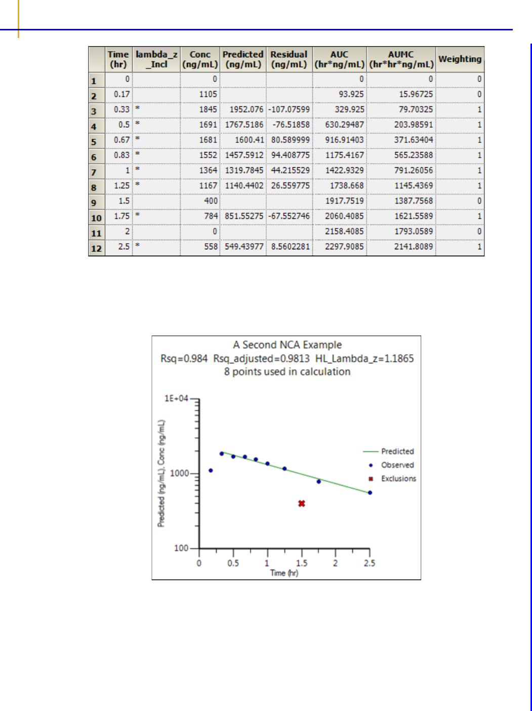
Phoenix WinNonlin

User’s Guide

166

Note that values used in the calculation of Lambda Z are marked with an asterisk in the column

Lambda_z_Incl. The data point corresponding to time 1.5, which was excluded manually, is not

marked with an asterisk. The observation at time 2.0, with a value of zero, was automatically

excluded.

4. Click Observed Y and Predicted Y vs X.

The excluded data point is marked on the Observed Y and Predicted Y vs X plot output of

observed and predicted data.

This concludes the partial areas example.

167

Sparse sampling NCA example

This example demonstrates how to model with sparse sampling. The time-concentration data is pro-

vided in

SparseSamplingChaioYeh.xls. The dosing and therapeutic response data are stored

SparseSamplingChaioYeh_sources.xls. These files are located in the Phoenix exam-

ples directory.

The completed project (

NCA_SparseSampling.phxproj) is available for reference in

…\Examples\WinNonlin.

Set up the NCA object

Create a project called NCA_SparseSampling.

2. Import the two files …\Examples\WinNonlin\Supporting files\SparseSam-

plingChaioYeh.xls

and SparseSamplingChaioYeh_sources.xls.

In the File Import Wizard dialog, select the Has units row option for Sheet 1 and Dosing work-

sheets.

3. Select Workflow in the Object Browser and then select Insert > NonCompartmental Analysis >

NCA.

4. Rename the NCA object just added as SparseSamplingChaioYeh.

5. Drag the SparseSamplingChaioYeh worksheet from the Data folder to the SparseSamplingC-

haioYeh object’s Main Mappings panel. Map the context as follows:

Subject set to None context

Time to Time context

Conc to Concentration context

Set up for sparse sampling

Select Dosing in the Setup list.

2. Expand the SparseSamplingChaioYeh_sources item in the Object Browser Data folder and drag

the Dosing item to the Dosing panel.

Type is already mapped to the None context.

Dose is already mapped to the Dose context.

Time is already mapped to the Time context.

3. Select Therapeutic Response in the Setup list.

4. In the expanded SparseSamplingChaioYeh_sources item in the Object Browser Data folder,

drag the TherapeuticResponse item to the Therapeutic Response panel.

Lower is already mapped to the Lower context.

5. In the Options tab, check the Sparse check box.

Execute and view the NCA results

All necessary settings are complete.

1. Click (Execute icon) to execute the object.

2. In the Results tab, click Final Parameters.

Phoenix WinNonlin

User’s Guide

168

Figure 23-1. Part of the Final Parameters worksheet

3. Click Summary Table.

4. Click Observed Y and Predicted Y vs X.

169

This concludes the sparse sampling example.

Phoenix WinNonlin

User’s Guide

170

Urine study NCA example

This example demonstrates how to model a urine study. The time range, concentration, and data is

provided in

urine.xls. The dosing data are stored in urine_sources.xls. These files are

located in the Phoenix examples directory.

The completed project (

NCA_UrineStudy.phxproj) is available for reference in …\Exam-

ples\WinNonlin

Set up the NCA object

Create a project called NCA_UrineStudy.

2. Import the two files …\Examples\WinNonlin\Supporting files\urine.xls and

urine_sources.xls.

In the File Import Wizard dialog, select the Has units row option for both worksheets.

3. Select Workflow in the Object Browser and then select Insert > NonCompartmental Analysis >

NCA.

4. Rename the NCA object just added as urine.

5. In the Options tab, set the Model Type to Urine (210-212).

6. Drag the urine worksheet from the Data folder to the urine object’s Main Mappings panel to map it

as the input source.

7. In the Main Mappings panel, map the data types to the following contexts:

Map Lower to the Start Time context.

Map Upper to the End Time context.

Leave Concentration mapped to the Concentration context.

Leave Volume mapped to the Volume context.

8. Select Dosing in the Setup list.

9. Drag the urine_sources item from the Data folder to the Dosing panel.

Type is already mapped to the None context.

Dose is already mapped to the Dose context.

Time is already mapped to the Time context.

10. Select Therapeutic Response in the Setup list.

11. In the Therapeutic Response panel, check the Use Internal Worksheet checkbox.

12. In the first cell of the Lower column, enter 4.

Execute and view the NCA results

All necessary settings are complete.

1. Click (Execute icon) to execute the object.

2. In the Results tab, click Final Parameters.

171

Figure 24-1. Part of the Final Parameters worksheet

3. Click Summary Table.

Values used in the calculation of Lambda Z are marked with an asterisk in the Lambda_z_Incl col-

umn.

4. Click Observed Y and Predicted Y vs X.

Phoenix WinNonlin

User’s Guide

172

This concludes the urine study example.

173

Drug effect NCA example

This example demonstrates how to model a urine study. The time range, concentration, and data are

provided in

nca_pd.xls. The dosing data are stored in nca_pd_sources.xls. These files are

located in the Phoenix examples directory.

The completed project (

NCA_DrugEffect.phxproj) is available for reference in …\Exam-

ples\WinNonlin

Set up the NCA object

Create a project called NCA_DrugEffect.

2. Import the two files …\Examples\WinNonlin\Supporting files\nca_pd.xls and

nca_pd_sources.xls.

In the File Import Wizard dialog, select the Has units row option for Sheet 1.

3. Select Workflow in the Object Browser and then select Insert > NonCompartmental Analysis >

NCA.

4. Rename the NCA object just added as nca_pd.

5. In the Options tab, set the Model Type to Drug Effect (220).

6. Drag the nca_pd worksheet from the Data folder to the nca_pd object’s Main Mappings panel to

map it as the input source.

Map Time to the X context.

Map Cortisol_RR to the Y context.

7. Select Dosing in the Setup list.

8. Expand the nca_pd_sources item in the Object Browser Data folder and drag the Dosing item to

the Dosing panel.

Type is already mapped to the None context.

Time is already mapped to the Time context.

9. Select Partial Areas in the Setup list.

10. In the expanded nca_pd_sources item in the Object Browser Data folder, drag the PartialAreas

item to the Partial Areas panel.

Map Curve to the Area # context.

Map Lower to the Start Time context.

Map Upper to the End Time context.

11. Select Parameter Names in the Setup list.

12. In the expanded nca_pd_sources item in the Object Browser Data folder, drag the Names item to

the Parameter Names panel.

Map Name to the Parameter Name context.

Leave Preferred mapped to the Preferred context.

Map Include to the Include in Workbook context.

13. Select Slopes in the Setup list and enter the following information:

For the first row:

60 for Start Time

67 for End Time

Time Range for Fit Method

Linear for Lin/Log



For the second row:

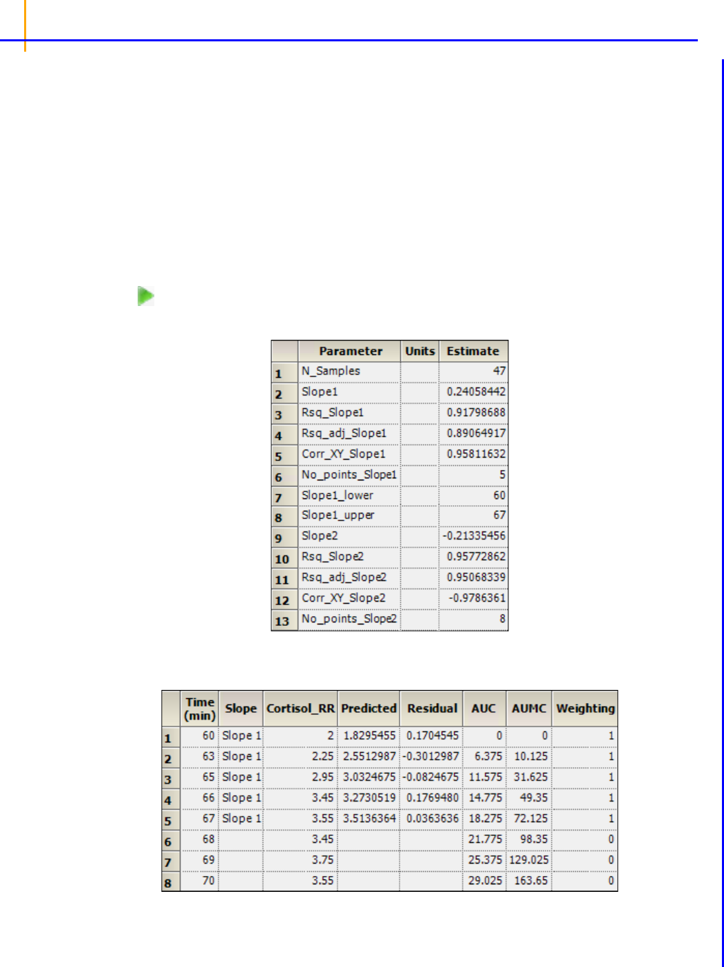
Phoenix WinNonlin

User’s Guide

174

125 for Start Time

133 for End Time

Time Range for Fit Method

Linear for Lin/Log

14. Select Therapeutic Response in the Setup list, check the Use Internal Worksheet box and enter

the following information:

2.5 for Baseline

5 for Threshold

Execute and view the NCA results

All necessary settings are complete.

15. Click (Execute icon) to execute the object.

16. In the Results tab, click Final Parameters.

Figure 25-1. Part of the Final Parameters worksheet

17. Click Summary Table.

This concludes the drug effect example.

175

Multiple profile analysis using NCA

Data for noncompartmental analyses can include one or more sort variables. Sort variables have

discrete values that identify time-concentration profiles to be analyzed individually. Input datasets

should be stacked (long and skinny) rather than unstacked (short and wide).

Stacking simply means moving information stored in column headings into the rows. For example,

matrix data such as plasma or urine can be placed in one row, and all associated data are arranged in

rows beside the matrix data. This means that all measurements appear in a single column, with one

or more additional columns flagging which data belong to which matrix. The data for one matrix must

be listed first, then all the data for the other matrix.

For noncompartmental analysis data, this means that time (the independent variable) and concentra-

tion (the dependent variable) data for all individuals should occupy only one column each, with one or

more additional columns (sort variables) used to identify individual profiles.

This example demonstrates the general steps to summarize a dataset using noncompartmental anal-

ysis. The dataset contains time-concentration profiles from a two period crossover study with six sub-

jects.

The study data for this example are contained in

Profiles.CSV, which is located in the Phoenix

examples directory. This crossover study includes two sort variables: Subject (subject identifiers) and

Form (formulation). There are six subjects, each of whom was tested with two formulations, for a total

of twelve profiles.The completed project (

Multiple_Profiles.phxproj) is available for refer-

ence in

…\Examples\WinNonlin.

Set up the project

Create a new project called Multiple Profiles.

2. Import the file …\Examples\WinNonlin\Supporting files\Profiles.CSV.

In the File Import Wizard dialog, select the Has units row option.

Review profile plots

Before analyzing the data, examine a plot of each profile to confirm the model and scan for outlying

data points.

1. Right-click Profiles in the Data folder and then select Send To > Plotting > XY Plot.

2. In the XY Data Mappings panel:

Map Subject to the Group context.

Map Form to the Lattice Conditions Page (Sort) context.

Map Time to the X context.

Map Conc to the Y context.

Note: The plot display options are located in the XY Plot's Options tab. Expand items in the Options

menu tree by clicking the (+) signs.

3. In the Options tab, with Plot selected in the menu tree, click the Title tab.

4. In the Title field type Plotting Multiple Profiles.

5. Click (Execute icon) to execute the object. 



There are two formulations in the input dataset. Since Form (formulation) was mapped to the Page

Phoenix WinNonlin

User’s Guide

176

(Sort) Lattice Condition context, two plots are generated, each representing a formulation, and

each on a separate tab. The plot for the first formulation (Capsule) is displayed automatically.

6. Click the Page 02 tab to view the plot for the second formulation (Tablet).

Set up the NCA object for the multiple profile analysis

The noncompartmental analysis (NCA) plasma model 200 (extravascular dosing) is suitable for this

data. All subjects had a dose of 100 ng at time zero for each formulation. All profiles use uniform

weighting, and allow Phoenix to select the terminal elimination phase. The linear trapezoidal method

with linear interpolation is used to compute the areas under the curve.

1. Right-click Profiles in the Data folder and select Send To > NonCompartmental Analysis >

NCA.

177

2. In the Main Mappings panel:

Map Subject to the Sort context.

Map Form to the Sort context.

Leave Time mapped to the Time context.

Map Conc to the Concentration context.

Prepare the dosing information from the multiple profiles

Select Dosing in the Setup list.

2. Check the Use Internal Worksheet checkbox.

Click OK in the Dosing sorts dialog to accept the default sort variables.

For each cell in the Time column, enter

0.

For each cell in the Dose column, enter

100. 

Do not enter any value in the Tau column.

3. In the Dose Options area of the Options tab, type ng in the Unit field and press the Enter key.

4. Extravascular is selected by default in the Type menu. Do not change this setting.

Add a partial area calculation

Select Partial Areas in the Setup list.

2. Check the Use Internal Worksheet checkbox.

Click OK in the Partial Areas sorts dialog to accept the default sort variables.

For each cell in the Start Time column, enter

0.

For each cell in the End Time column, enter

120.

Specify the NCA model options for the multiple profile analysis

In the Options tab, the default setting for Model Type is Plasma (200-202). Do not change this

setting.

Note: The exact plasma model type (200, 201, or 202) is determined by the dose type.

2. The default setting for Calculation Method is Linear Trapezoidal Linear Interpolation. Do not

change this setting.

3. In the Titles field type Processing Multiple Profiles with Model 200.

Set up a user-defined parameter

Go to the User Defined Parameters tab.

2. Check the Include with Final Parameters checkbox.

3. Enter 75 in the field to compute the concentration at 75 minutes.

Phoenix WinNonlin

User’s Guide

178

Execute and view the results of the multiple profile analysis

At this point, all of the necessary mappings and options have been specified.

1. Execute the object. 



In each Results worksheet, the sort variables Subject and Form are included as columns in the

data grid, and the output is presented for each level of the sort variables. See the NCA

“Results”

for descriptions of the output.

2. Select the Observed Y and Predicted Y vs X plot in the Results tab and double-click it. The plot

is opened in its own window.

3. In the Options menu tree below the plot, select Lattice under Plot.

4. Clear the Bind Lattice to Data checkbox.

5. Click the up and down arrows in the Lattice Rows and Lattice Columns boxes to change the

number of rows/columns, respectively, that form the lattice.

6. Close the Observed Y and Predicted Y vs X window.

Phoenix can display a maximum of 15 latticed rows and 15 latticed columns, but no more than 200

charts per page. The number of plots that can be displayed per page depends on the monitor size and

resolution. If too many plots are placed on one page the axes labels, legends, and other plot informa-

tion can be difficult to read. Additional information on lattices can be found in

“More on latticed plots in

Phoenix”

Summarize the multiple profile analysis output with statistics

Phoenix's Descriptive Statistics object is used to summarize several of the output parameters in the

Final Parameters Pivoted worksheet. The Descriptive Statistics object generates separate statistics

for each formulation.

1. Right-click Workflow in the Object Browser and select New > Computation Tools > Descriptive

Statistics.

2. In the Descriptive Statistics Main Mappings panel click (Select Source icon).

3. In the dialog, under the NCA node, select the Final Parameters Pivoted worksheet and click OK.

4. Map:

Form to the Sort context.

Tmax, Cmax, and AUCall to the Summary context.

Leave all other data types mapped to None.

5. In the Options tab, check the Confidence Intervals and Number of SD Statistics checkboxes,

but do not change the default values for these two items.

6. Execute the object.

This example summarizes

AUCall, the area under the curve through the last measured value,

Cmax, the maximal concentration of drug in the blood, and Tmax, the time at maximal concentration.

179

Create a Cmax plot with error bars

This section will illustrate how to use the means and SDs of data, computed by the Descriptive Statis-

tics object, to create an overlaid plot with error bars. The Descriptive Statistics results obtained in the

previous section will be filtered so that the output for only one variable (Cmax) remains. The data will

then be used to create the error bars for a plot of Cmax values.

First filter the Descriptive Statistics results:

1. Right-click Workflow in the Object Browser and select New > Data Management > Data Wizard.

2. In the Options tab, select Filter from the Action menu and click Add right below the menu.

3. Click the Select Source icon in the Mappings panel.

4. In the Select Source dialog, under the Descriptive Statistics node, select Statistics, and click

OK.

Phoenix WinNonlin

User’s Guide

180

5. In the Options tab, click the Add button to the right of the Specify Filter field.

6. In the Filter Specification dialog, select Include as the Action.

7. Type Cmax in the Select Column or Enter Value field.

8. Make sure the Apply to entire row box is checked.

9. Click OK.

10. Execute the object.

The Result worksheet now only contains the rows of Cmax data.

Now set up the X-Categorical XY Plot object:

1. Right-click Workflow in the Object Browser and select New > Plotting > X-Categorical XY Plot.

2. Click the Select Source icon in the Mappings panel and select the NCA Final Parameters Piv-

oted worksheet and click OK.

3. Map:

Form to the X context.

Cmax to the Y context.

Leave all other data types mapped to None.

4. In the Options tab, select Plot in the menu tree and then the Graphs sub-tab.

5. Click the Add button.

6. Select the CategoricalX 1 Data item in the Setup tab, click the Select Source icon.

7. In the Select Source dialog, under the Data Wizard node, select Result, and click OK.

8. Map:

Form to the X context.

Mean to the Y context.

SD to both the Error Bars Lower and Upper contexts.

Adjust the appearance of the plot:

1. In the Options tab, with Plot selected in the menu tree, go to the Title sub-tab.

2. Enter Cmax Results per Formulation with Mean and Std Dev in the field and

click the icon to center the plot title.

3. In the menu tree, select Cmax vs Form under the Graphs node.

4. Change the Marker Color to Red and set the Marker Size to 7.

5. Select Mean vs Form under the Graphs node.

6. In the Content sub-tab, check the Offset checkbox and enter 14 for the number of pixels.

7. Select the Appearance sub-tab and set the Marker Shape to Triangle.

8. In the menu tree, expand the Mean vs Form node and select Error Bars.

9. Click the Appearance sub-tab and set the Color to Red and the Cap Width to 9.

10. Execute the object.

The output is an overlay of two graphs (Cmax vs Form and Mean vs Form) that includes error bars.

181

Export results to Microsoft Word

The results of any operational object can be exported to a Microsoft Word document. This example

shows how to format plot output and export it to Microsoft Word. By default, plots are exported at a

resolution of 1024 by 768 pixels.

1. Select File > Word Export.

2. In the Word Export dialog, click the (+) signs beside Workflow > NCA > Results to expand the

menu tree.

3. Select the Observed Y and Predicted Y vs X checkbox.

4. Select the Summary Table checkbox.

Phoenix WinNonlin

User’s Guide

182

5. Click Options.

6. Select the Landscape option button in the Document tab.

7. Make sure the Add source line to objects checkbox is cleared and click Finished.

8. Click Export.

Phoenix creates a new Microsoft Word document and exports the selected objects into the docu-

ment.

9. In the Export Complete dialog, click OK.

10. Save the Word file and exit Microsoft Word.

11. Close the project by right-clicking the project in the Object Browser and selecting Close Project.

NonParametric Superposition

183

NonParametric Superposition

In pharmacokinetics it is often desirable to predict the drug concentration in blood or plasma after mul-

tiple doses, based on concentration data from a single dose. This can be done by fitting the data to a

compartmental model with some assumptions about the absorption rate of the drug. An alternative

method is based on the principle of superposition, which does not assume any pharmacokinetic (PK)

model.

Phoenix’s nonparametric superposition object is used to predict drug concentrations after multiple

dosing at steady state, and is based on noncompartmental results describing single dose data. The

predictions are based upon an accumulation ratio computed from the terminal slope (Lambda Z). The

feature allows predictions from simple (the same dose given in a constant interval) or complicated

dosing schedules. The results can be used to help design experiments or to predict outcomes of clini-

cal trials when used in conjunction with the semicompartmental modeling function.

Use one of the following to add the object to a Workflow:

Right-click menu for a Workflow object: 

New > NonCompartmental Analysis > Nonparametric Superposition 

Main menu: 

Insert > NonCompartmental Analysis > Nonparametric Superposition

Right-click menu for a worksheet: 

Send To > NonCompartmental Analysis > Nonparametric Superposition

Note: To view the object in its own window, select it in the Object Browser and double-click it or press

ENTER. All instructions for setting up and execution are the same whether the object is viewed in

its own window or in Phoenix view.

User interface description

Results

NonParametric Superposition methodology

NonParametric Superposition example

User interface description

Main Mappings panel

Administered Dose panel

Terminal Phase panel

Dosing panel

Options tab

Plots tab (See the

“Plots tab” description in the NCA section.)

Main Mappings panel

Use the Main Mappings panel to identify how input variables are used in the NonParametric object.

NonParametric superposition requires a dataset containing time and concentration data, and sort vari-

ables to identify individual profiles. Required input is highlighted orange in the interface.

None: Data types mapped to this context are not included in any analysis or output.

Sort: Categorical variable(s) identifying individual data profiles, such as subject ID in a nonpara-

metric analysis. A separate analysis is performed for each unique combination of sort variables.

Time: The relative or nominal sampling times used in a study.

Concentration: The measured amount of a drug in blood plasma.

Phoenix WinNonlin

User’s Guide

184

Administered Dose panel

Using the Administered Dose panel is optional. When this panel is not used, it is assumed that the

administered dose, or the dose associated with the data, is the same as the Loading Dose specified

in the Regular Dosing tab, or the same as the dose at time zero specified in the Variable Dosing tab.

Required input is highlighted orange in the interface.

Note: The sort variables in the dosing data worksheet must match the sort variables used in the main

input dataset.

None: Data types mapped to this context are not included in any analysis or output.

Sort: Categorical variable(s) identifying individual data profiles, such as subject ID in a nonpara-

metric analysis. A separate analysis is performed for each unique combination of sort variables.

Administered Dose: The amount of drug given.

Terminal Phase panel

A dataset containing terminal phase information is options. If the dataset is available, use the Termi-

nal Phase panel for mapping the start and end times for the terminal elimination phase for each pro-

file. Use an internal worksheet to set the range (NPS does not use an extern worksheet mapping for

Lambda Z setup.)

Note: The sort variables in the dosing data worksheet must match the sort variables used in the main

input dataset.

None: Data types mapped to this context are not included in any analysis or output.

Sort: Categorical variable(s) identifying individual data profiles, such as subject ID in a nonpara-

metric analysis. A separate analysis is performed for each unique combination of sort variables.

Start and End: Start and end times for the terminal elimination phase. These contexts are gener-

ally not required. However, if the user maps an external worksheet to Terminal Phase, then the

Start and End columns are required.

Dosing panel

The Dosing panel is only available if Variable is selected in the Dosing type menu. If the main input

dataset used with the nonparametric superposition object contains variable times between doses,

then use the Dosing panel to enter the separate time and dose values. Required input is highlighted

orange in the interface.

None: Data types mapped to this context are not included in any analysis or output.

Time: Time that the drug is administered. 

Dose: The amount of drug administered.

Options tab

The Options tab allows users to select the dosing type, specify options related to regular and variable

dosing, and enter dosing values for regular dosing.

NonParametric Superposition

185

• In the Dosing Type menu, select the dosing interval type.

Regular: For dosing at a regular time interval.

Variable: For dosing at variable time intervals.

If variable dosing is selected then the Dosing panel is displayed in the Setup tab list. The Dosing

panel is used to enter separate doses and times.

Selecting different dosing type changes the options in the Options tab. For regular dosing type

options see

“Regular dosing options”. For variable dosing type options see “Variable dosing

options”

• In the Number of data output points field, type the number of data output points.

The default number of data points for regular dosing is 101. The default number of data points for

variable dosing is 1001.

• In the Method for computations menu, select the method used for interpolation and extrapola-

tion of untransformed data.

Linear: Uses only Linear interpolation. Use when data after Tmax is not necessarily exponentially

declining.

Linear/Log: For each dosing interval, uses Linear interpolation through the Tmax of that interval,

and Log interpolation after Tmax.

Regular dosing options

• In the Loading Dose field, type the initial dose used to calculate the AUC (area under the curve).

• In the Maintenance dose field, type the maintenance dose used to calculate the AUC.

• In the Tau field, type the dosing interval value.

Note: The value entered in the Tau field must match the time values used in the dataset. For example, if

the time in the dataset is measured in hours and a dose is given once every day, type 24 in the Tau

field.

• Select the Display at steady state option button to have Phoenix generate the Predictions vs

Time plot at steady state.

• Select the Display N

dose option button to have Phoenix generate the Predictions vs Time at a

particular dose.

• In the Display N

dose field, type the dose used to generate the Predictions vs Time plot.

Variable dosing options

• Select the Repeat every N time units checkbox to specify a repeating dosing regimen.

• In the Repeat every N time units field, type the repeat time for one dosing cycle.

Note: The time units entered in the Repeat every N time units field must match the time units used in

the Dosing panel. For example, if the dosing cycle repeats every 24 hours, type 24 in the Repeat

every N time units field.

• In the Output time range fields, type the start and end times used to create the predicted output

data.

Phoenix WinNonlin

User’s Guide

186

Results

NonParametric superposition generates worksheets containing predicted concentrations and Lambda

Z values, as well as plots of predicted concentration over time for each sort level, and a summary plot.

• The Concentrations worksheet contains times and predicted concentrations for each level of

the sort variables. If a regular dosing schedule is selected, this output represents times and

concentrations between two doses at steady state. If a variable dosing schedule is selected,

the output includes the times and concentrations within the supplied output range.

• The Lambda Z worksheet contains the Lambda Z value and the half-life for each sort key.

Note: NPS and NCA Best-Fit Lambda Z calculations can generate slightly different Lambda Z values (at

the sixth significant digit) when the input data contains eight significant digits or more.



NPS stops if the last three points fail to compute Lambda Z (such as the last three points going

uphill). If this situation occurs, you can execute NCA on the data using the default settings, and

then map the NCA Slopes result to the Terminal Phase setup in the NPS object. The NCA execu-

tion will check further back in the dataset to see if a larger group of points ending with the last point

will yield a valid Lambda Z.

NonParametric Superposition methodology

NonParametric superposition assumes that each dose of a drug acts independently of every other

dose; that the rate and extent of absorption and average systemic clearance are the same for each

dosing interval; and that linear pharmacokinetics apply, so that a change in dose during the multiple

dosing regimen can be accommodated.

In order to predict the drug concentration resulting from multiple doses, one must have a complete

characterization of the concentration-time profile after a single dose. That is, it is necessary to know

C(t

) at sufficient time points t

, (i=1,2,…,n), to characterize the drug absorption and elimination pro-

cess. Two assumptions about the data are required: independence of each dose effect, and linearity

of the underlying pharmacokinetics. The former assumes that the effect of each dose can be sepa-

rated from the effects of other doses. The latter, linear pharmacokinetics, assumes that changes in

drug concentration will vary linearly with dose amount.

The required input data are the time, dosing, and drug concentration. The drug concentration at any

particular time during multiple dosing is then predicted by simply adding the concentration values as

shown in the next section (

“Computation method”).

Note: User-defined terminal phases apply to all sort keys. In addition, dosing schedules and doses are

the same for all sort keys.

Computation method

Given the concentration data points C(t

) at times t

, (i=1,2,…,n), after a single dose D, one may

obtain the concentration

C(t) at any time t through interpolation if t

< t <t

, or extrapolation if t > t

The extrapolation assumes a log-linear elimination process; that is, the terminal phase in the plot of

log(

C(t)) versus t is approximately a straight line. If the absolute value of that line’s slope is 

and

the intercept is ln(

), then C(t) = exp(–

t) for (t > t

The slope



and the intercept are estimated by least squares from the terminal phase; the time

range included in the terminal phase may be specified by the user or, if not specified, estimates from

t

-----





Ct 

–=

Conc t C

jt



12 m,,,==

t C

t  t +–t 2+–

 tn1–+–

t  t +–

1  n 1––exp–

1 –exp–

--------------------------------------------------

exp+=

exp++

exp+exp+=

t C

t 

 t +–

1 –exp–

-------------------------------------exp+=

Ct Ct

i 1–

Ct

i 1–

–

i 1–

–

i 1–

–

--------------------

i 1–



NonParametric Superposition

187

the best linear fit (based on adjusted R

as in the Best Fit method in Noncompartmental Analysis) will

be used. The half life is: ln(2)/



Suppose there are m additional doses D

, j = 1,…,m, and each dose is administered after 

time

units from the first dose. The concentration due to dose

will be:

where t is time since the first dose and C(t – 

) = 0 for t  

The total predicted concentration at time

t will be:

If the same dose is given at constant dosing intervals

, and  is sufficiently large that drug concentra-

tions reflect the post-absorptive and post-distributive phase of the concentration-time profile, then

steady state can be reached after sufficient time intervals. Let the concentration of the first dose be

(t) for 0 < t < , so  is greater than t

. Then the concentration at time t after n

dose (i.e., t is rela-

tive to dose time) will be:

As , the steady state (

ss) is reached:

To display the concentration curve

at steady state, Phoenix assumes steady state is at ten times the

half life.

For interpolation, Phoenix offers two methods: linear interpolation and log-interpolation. Linear inter-

polation is appropriate for log-transformed concentration data and is calculated by:

n 

Ct Ct

i 1–

Ct



i 1–

log–

log



i 1–

–

i 1–

–

--------------------

+log













i 1–

,

exp=

Phoenix WinNonlin

User’s Guide

188

Log-interpolation is appropriate for original concentration data, and is evaluated by:

For additional information see Appendix E of Gibaldi and Perrier (1982). Pharmacokinetics, 2nd ed.

Marcel Dekker, New York.

NonParametric Superposition example

This example uses the output from the semicompartmental modeling example, detailed under “Semi-

compartmental model example”. The study data are from an early Ph

ase I PK/PD trial. Quick input is

sought for the design of a seven day multiple dose study. However, the profiles are irregular, and it is

not easy to apply a compartmental modeling approach to the data.

This section uses the NonParametric Superposition object to predict plasma concentrations and

effect-site concentrations at steady-state based on single-dose data. This feature allows for predic-

tions on data that are otherwise difficult to model.

Knowledge of how to do basic tasks using the Phoenix interface, such as creating a project and

importing data, is assumed.

The completed project (

NPS.phxproj) is available for reference in …\Examples\WinNonlin.

Set up an estimation of steady-state plasma concentrations

1. Create a projec

t called NPS.

2. Import the files

…\Examples\WinNonlin\Supporting files\SCM_Results.xls.

In the File Import Wizard dialog, select the Has units row option.

1. Right-click SC

M_Results in the Data folder and select Send To > NonCompartmental Analysis

> NonParametric Superposition.

2. In the Main Mappings panel:

p Subject to the Sort context.

Leave Time mapped to the Time context.

Map Conc to the Concentration context.

Leave Ce mapped to None.

Leave Effect mapped to None.

3. In the Options tab below the Setup panel, type

50 in the Loading Dose field.

4. In the Ma

intenance Dose field type 50.

5. In the Ta

u (dosing interval) field type 4.

Execute and view the plasma estimation results

1. Click (Execute icon)

to execute the object.

NonParametric Superposition

189

The Concentration worksheet provide predicted steady-state plasma concentrations. The Lambda z

worksheet lists the Lambda Z and half-life estimates.

The plot output shows predicted steady state concentrations over time for each subject. The first sub-

ject’s plot is shown below.

Set up an estimation of steady-state effect-site concentrations

Select the NonParametric object’s Setup panel.

2. In the Main Mappings panel, re-map the data types to the following contexts:

Leave Subject mapped to the Sort context.

Leave Time mapped to the Time context.

Map Conc to None.

Map Ce to the Concentration context.

Leave Effect mapped to None.

3. Select Terminal Phase from the Setup list.

4. Check the Use Internal Worksheet checkbox.

5. For each row:

In the Start column, type

4. 

In the End column, type

Execute and view the effect-site concentration estimation results

Execute the object.

Phoenix WinNonlin

User’s Guide

190

The new NonParametric worksheet results provide predicted effect site concentrations at steady-

state and Lambda Z and half-life estimates.

The plot output shows predicted effect site concentrations at steady-state over time for each subject.

The first subject’s graph is shown below.

Compute the steady-state effect

Now it is possible to compute the steady-state effect from the predicted steady-state concentrations at

the effect site.

In the Semicompartmental example, the PD model 103 was used (its sample graph is shown below).

The effect formula for model 103 is E=E0*(1 – (C/(C+IC50))). This formula will be adjusted for each

subject in the study.

1. In the Results tab, right-click the Concentrations (effect site concentrations) worksheet and select

Copy to Data Folder.



The worksheet is added to the project’s Data folder and renamed “Concentrations from NonPara-

metric”.

2. In the Object Browser, select Concentrations from NonParametric in the Data folder.

3. In the Columns tab below the table, click Add under the Columns list.

NonParametric Superposition

191

4. In the New Column Properties dialog, the Numeric option button is selected by default. Do not

change this setting.

5. In the Column Name field type Effect and click OK.



The Effect column is added in the Columns list and in the table in the Grid tab.

6. Use the Down Arrow button beside the Columns list to move the Effect column header to the bot-

tom of the Columns list.

7. In the Object Browser, right-click Concentrations from NonParametric and select Edit in Excel.



Phoenix displays a message warning users that changes made in Excel are not recorded in Phoe-

nix.

8. Click OK.



The worksheet is opened in Excel. If you see a pop-up dialog stating that the format and extension

of the file do not match, click Yes to continue as the file is safe to open. 



In Excel, enter the PD model 103 effect formula in the Effect column for each subject at time zero.

Use the E0 and IC50 values from the PD Model object’s Final Parameters worksheet.

9. Select the cell in the Effect column at time zero for the first subject, JDW.

10. Type the effect formula shown below in the Effect column cell at time 0 (zero) for subject JDW,

which is row 3.

= 102.93*(1-(C3/(C3+0.09))) (for subject JDW)

11. Repeat for the second and third subjects, LEJ (row 104) and SCC (row 205).

= 100.17*(1-(C104/(C104+0.09))) (for subject LEJ)



= 100.45*(1-(C205/(C205+0.08))) (for subject SCC)

12. After the Effect value formula is set up at time zero for each subject copy the formula to the other

time points for each subject.



Because of the way Phoenix handles its interactions with Excel, users cannot use the Save As

option in Excel to save the worksheet with a different name or to a different location. The Save

option must be used.

13. Select File > Save.

14. Close Excel. Be sure to save the worksheet before closing Excel, or all changes are lost. 

An Apply Changes message dialog is displayed.

15. Click Yes to apply the changes. An entry is written in the worksheet History tab noting that it was

edited in Excel.

16. When asked whether to save formulas, select No so that the worksheet is editable in Phoenix.



The Concentrations from NonParametric worksheet now has Effect values derived from the equa-

tions used in the Excel edit and can still be used with operational objects.

Plot time vs effect

Once the steady-state effects and concentrations are generated it is possible to use the modified con-

centrations from NonParametric worksheet to plot time vs. effect for each subject by mapping the

worksheet to an XY Plot object.

Phoenix WinNonlin

User’s Guide

192

1. Right-click Concentrations from NonParametric in the Data folder and select Send To > Plot-

ting > XY Plot.

2. In the XY Data Mappings panel:

Map Subject to the Group context.

Map Time to the X context.

Leave Ce mapped to None.

Map Effect to Y context.

3. Execute the object.

This concludes the Nonparametric superposition example.

Semicompartmental Modeling

193

Semicompartmental Modeling

Semicompartmental modeling was proposed by Kowalski and Karim (1995) for modeling the temporal

aspects of the pharmacokinetic-pharmacodynamic relationship of drugs. Their model was based on

the effect-site link model of Sheiner, Stanski, Vozeh, Miller and Ham (1979) to estimate effect-site

concentration

, but uses a piecewise linear model for plasma concentration C

rather than specify-

ing a PK model for

. The potential advantage of this approach is reducing the effect of model mis-

specification for

when the underlying PK model is unknown.

Use one of the following to add the object to a Workflow:

Right-click menu for a Workflow object: 

New > NonCompartmental Analysis > Semicompartmental Modeling. 

Main menu: 

Insert > NonCompartmental Analysis > Semicompartmental Modeling.

Right-click menu for a worksheet: 

Send To > NonCompartmental Analysis > Semicompartmental Modeling.

Note: To view the object in its own window, select it in the Object Browser and double-click it or press

ENTER. All instructions for setting up and execution are the same whether the object is viewed in

its own window or in Phoenix view.

User interface description

Results

Semicompartmental calculations

Semicompartmental model example

User interface description

Main Mappings panel

Options tab

Plots tab (See the

“Plots tab” description in the NCA section.)

Main Mappings panel

Use the Main Mappings panel to identify how input variables are used in the Semicompartmental

object. Semicompartmental modeling requires a dataset containing time and concentration data, and

sort variables to identify individual profiles. Required input is highlighted orange in the interface.

None: Data types mapped to this context are not included in any analysis or output.

Sort: Categorical variable(s) identifying individual data profiles, such as subject ID in a semicompart-

mental analysis. A separate analysis is performed for each unique combination of sort variables.

Time: The relative or nominal dosing times used in a study.

Concentration: The measured amount of a drug in blood plasma.

Effect: The measured effect data.

Phoenix WinNonlin

User’s Guide

194

Options tab

The Options tab allow users to select the computation method and the Ke0 value.

•In the Computation Method menu, select the method Phoenix uses to perform the semicompart-

mental analysis.

Linear uses a linear piecewise PK model.

Log uses a log-linear piecewise PK model.

Linear/Log start with linear to Tmax and then log-linear after Tmax; this is also the default option.

• In the Ke0 field, type the value for the equilibrium rate constant.

Results

The Semicompartmental model object generates four charts, one worksheet, and one text file.

Up to four plots are created for each profile. Each profile’s plot is displayed on its own page in the

Results tab. Click the page tabs at the bottom of each plot panel to view the plots for individual pro-

files. If drug effect data is included in the dataset,

Effect vs Ce and Effect vs Cp plots are also cre-

ated.

Ce vs Time: Estimated effect site concentration vs. time.

Cp vs Time: Plasma concentration vs. time.

Effect vs Ce: Drug effect vs. the estimated effect site concentration.

Effect vs Cp: Drug effect vs. plasma concentration.

A text file called Settings is also created. It lists the user-specified settings in the Semicompartmental

object

The Semicompartmental object creates a worksheet called Results. This worksheet contains: sort

variables (if any are used), time points used in the study, drug concentration levels in blood plasma,

Ce (estimated effect site concentration), effect data (if included). Any units associated with the time

and concentration columns in the input data are carried through to the semicompartmental modeling

output.

Semicompartmental calculations

Phoenix’s semicompartmental modeling estimates effect-site concentrations for given times and

plasma concentrations and an appropriate value of

. This function should be used when a coun-

terclockwise hysteresis is observed in the graph of effect versus plasma concentrations. The hystere-

sis loop collapses with the graph of effect versus effect-site concentrations.

A scientist developing a PK/PD link model based upon simple IV bolus data can use this function to

compute effect site concentrations from observed plasma concentrations following more complicated

administration regimen without first modeling the data, i.e., semicompartmental modeling determines

if the hysteresis can be collapsed using an effect compartment, without requiring a full compartmental

model. The results can then be compared to the original datasets to determine if the model suitably

describes pharmacodynamic action after the more complicated regimen.

Semicompartmental Modeling

195

Data and assumptions

Drug concentration in plasma C

for each subject is measured at multiple time points after the drug is

administrated. To minimize the bias in estimating

, the time points need to be adequately sampled

such that accurate estimation of the AUC by noncompartmental methods can be obtained. Effect-site

link model is used and the value of the equilibration rate constant

that accounts for the lag

between the

and the C

curves is required. The default option is for a piecewise Linear/Log model

to be assumed for

Computation method

---------

–=

t C

j 1–



j 1–

– t

j 1–

+=

j 1–

––

j 1–



--------

–







1 e

j 1–

––

–



j 1–

–

t C

j1–

–

j 1–

–exp t

j 1–

=

In the effect-site link model proposed by Sheiner, Stanski, Vozeh, Miller and Ham (1979), a hypotheti-

cal effect compartment was proposed to model the time lag between the PK and PD responses. The

effect site concentration

is related to C

by first-order disposition kinetics and can be obtained by

solving the differential equation:

where

is a known constant. In order to solve this equation, one needs to know C

as a func-

tion of time, which is usually given by compartmental PK models.

Here, use a piecewise linear model for

where:

nd:

Using the above two equations can lead to a recursive equation for

The initial condition is

(0)=C

(0) =0.

One can also assume a log-linear piecewise PK model for



j 1–

–t

j 1–

–=

j1–

j 1–

=

Phoenix WinNonlin

User’s Guide

196

where:

and:



and are estimated by a linear regression, assuming C

(0) = C

(0) = 0.

Phoenix provides three methods. The ‘linear’ method uses linear piecewise PK model; the ‘log’

method uses log-linear piecewise PK model; the default ‘log/linear’ method uses linear to Tmax and

then log-linear after Tmax. The Effect field is not used for the calculation of

but when it is provided,

the

E vs C

and E vs C

plots will be plotted.

References

Kowalski ad Karim (1995). A semicompartmental modeling approach for pharmacodynamic data

assessment, J Pharmacokinet Biopharm 23:307–22.

Sheiner, Stanski, Vozeh, Miller and Ham (1979). Simultaneous modeling of pharmacokinetics and

pharmacodynamics: application to d-tubocurarine. Clin Pharm Ther 25:358–71.

Semicompartmental model example

This example uses the dataset in the file PK.CSV, which is located in the Phoenix examples direc-

tory. The data are from an early Phase I PK/PD trial. Quick input is sought for the design of a seven

day multiple dose study. However, the profiles are irregular, and it is not easy to apply a compartmen-

tal modeling approach to the data. A semicompartmental approach will be attempted here. This

example then continues with a NonParametric Superposition prediction of plasma concentrations and

effect-site concentrations at steady-state, using the Semicompartmental results (see

“NonParametric

Superposition example”

Knowledge of how to do basic tasks using the Phoenix interface, such as creating a project and

importing data, is assumed.

The completed project (

SCM.phxproj) is available for reference in …\Examples\WinNonlin.

Explore the input data

Create a new project called SCM.

2. Import the file …\Examples\WinNonlin\Supporting files\PK.CSV.

In the File Import Wizard dialog, select the Has units row option.



The braces in the Effect column header indicate that the units are nonstandard and will be carried

throughout the analysis but they cannot be used in unit conversions.



j1–

ln C

ln–

j 1–

–

-------------------------------------------

j 1–

––

j 1–



–

-------------------



j 1–

––

j 1–

––

–+

Semicompartmental Modeling

197

3. Right-click PK in the Data folder and select Send To > Plotting > XY Plot.

4. In the XY Data Mappings panel:

Map Subject to the Group context.

Map Time to the X context.

Map Conc to the Y context.

Leave Effect mapped to None.

5. Click (Execute icon) to execute the object. 



The plot indicates that compartmental modeling might be problematic. The data are highly vari-

able.

6. Return to the Setup panel and re-map the input data:

Leave Subject mapped to the Group context.

Map Time to None.

Map Conc to the X context.

Map Effect to the Y context.

7. In the Options tab below the Setup panel, select Graphs > Effect vs Conc in the menu tree.

8. Clear the Sort X Values checkbox.



Clearing the Sort X Values checkbox tells Phoenix to not sort the dataset by ascending concentra-

tion values before creating the XY plot.

9. Execute the object.

Phoenix WinNonlin

User’s Guide

198

Notice the hysteresis in the plot. Semicompartmental modeling supports calculation of effect-site

concentrations based on Ke0. In this example, pre-clinical studies indicated that the Ke0 is

between 0.2 and 0.3 per hour in rats and dogs.

Set up the Semicompartmental object

This example estimates effect-site concentrations using semicompartmental modeling:

1. Right-click PK in the Data folder and select Send to > NonCompartmental Analysis > Semi-

compartmental Modeling.

2. In the Main Mappings panel:

Map Subject to the Sort context.

Leave Time mapped to the Time context.

Map Conc to the Concentration context.

Leave Effect mapped to the Effect context.

3. In the Options tab below the Setup panel, type 0.25 in the Ke0 field.

Execute and view the Semicompartmental results for the PK data

Execute the object.

The Semicompartmental Model provides both workbook and graph output.

The Results worksheet shows the calculated concentration of the drug in the effect compartment, Ce,

at each Time in the input dataset, along with the input Conc and Effect data, for each subject.

Semicompartmental Modeling

199

Figure 28-1. Part of the Semicompartmental Results worksheet

The Semicompartmental object generated four plots for each subject.

Figure 28-2. Effect-compartment concentration (Ce) over time (Ce vs Time)

Phoenix WinNonlin

User’s Guide

200

Figure 28-3. Concentration over time (Cp vs Time)

Figure 28-4. Effect as a function of Ce (Effect vs Ce)

Semicompartmental Modeling

201

Figure 28-5. Effect over concentration (Effect vs Cp)

Based on the plots, PD model 103, an Inhibitory Effect E0 model, is appropriate to use to model the

concentration in the effect compartment (Ce) versus effect relationship.

Model the pharmacodynamics

Right-click Workflow in the Object Browser and select New > Modeling > Least Squares

Regression Models > PD Model.

2. Use the Select Source icon to map the Semicompartmental Results worksheet as the input

source for the PD Model object.

3. In the Mappings panel:

Map Subject to the Sort context.

Leave Time mapped to None.

Leave Conc mapped None.

Map Ce to the X variable context.

Map Effect to the Y variable context.

4. In the Model Selection tab below the Setup panel, check the model Number 103 checkbox.



The default model parameter options are used. Phoenix generates initial parameter values and

parameter bounds. To view the parameter option settings, select the Parameter Options tab.

Execute and view the PD Model results for the Semicompartmental output

Execute the object.



Phoenix analyzes each subject separately and includes all time points per subject.



The Final Parameters output provides estimates for E0 and IC50 for each subject. These are used

later to predict steady-state effect values.

Phoenix WinNonlin

User’s Guide

202

2. Click Observed Y and Predicted Y vs X under Plots.



The Observed Y and Predicted Y vs X plot illustrates the fit of PD model 103 to the effect data

when Ce from Semicompartmental modeling is used as the measure of exposure. The Observed

Y and Predicted Y vs X plot for the first subject is shown below.

The other plots address model fit.

The NonParametric superposition example uses the output from this example. You may wish to save

this project or leave the project open if you are continuing with the NonParametric superposition

example.

203

Modeling

Least-Squares Regression Models interface

Least-Squares Regression Models Results

Nonlinear Regression Overview

Least-Squares Regression Model calculations

Least-Squares Regression models include the following. Many of the models can be run using the

NLME engine (even if you do not have an NLME license). This is done by setting up a Maximum Like-

lihood Models object for individual modeling and using the Set WNL Model button to select the

model. See

“PK model options” in the Phoenix NLME documentation for more information. Refer to

“An example of individual modeling with Maximum Likelihood Model object” for an illustration of how a

dataset can be fitted to a two-compartment model with first-order absorption in the pharmacokinetic

model library using either the Least-Squares Regression PK Model or a Maximum Likelihood Model

object GUI.

Dissolution Models

Choose from Hill, Weibull, Double Weibull, or Makoid-Banakar dissolution models.

Indirect Pharmacodynamic Response Models

Four basic models have been developed for characterizing indirect pharmacodynamic responses

after drug administration. These models are based on the effects (inhibition or stimulation) that

drugs have on the factors controlling either the input or the dissipation of drug response. See

“Indirect Response models” for more details.

Linear Models

Phoenix includes a selection of models that are linear in the parameters. See

“Linear models” for

more details on available models. Refer to

“Linear Mixed Effects” for more sophisticated linear

models.

Michaelis-Menten Models

Phoenix’s Michaelis-Menten models are one-compartment models with intravenous or 1st order

absorption, and can be used with or without a lag time to the start of absorption. For more on

Phoenix’s Michaelis-Menten models, see

“Michaelis-Menten models”. Information on required

constants is available in

“Dosing constants for the Michaelis-Menten model”.

Pharmacodynamic Models

Phoenix includes a library of eight pharmacodynamic (PD) models. The PD models include sim-

ple and sigmoidal Emax models, and inhibitory effect models. For more on Phoenix’s PD models,

see

“Pharmacodynamic models”.

Pharmacokinetic Models

Phoenix includes a library of nineteen pharmacokinetic (PK) models. The PK models are one to

three compartment models with intravenous or first-order absorption, and can be used with or

without a lag time to the start of absorption. For more on Phoenix’s PK models, see

“Pharmacoki-

netic models”

. See also the “PK model examples”.

PK/PD Linked Models

When pharmacological effects are seen immediately and are directly related to the drug concen-

tration, a pharmacodynamic model is applied to characterize the relationship between drug con-

centrations and effect. When the pharmacologic response takes time to develop and the

observed response is not directly related to plasma concentrations of the drug a linked model is

usually applied to relate the pharmacokinetics of the drug to its pharmacodynamics.

Phoenix WinNonlin

User’s Guide

204



The PK/PD linked models can use any combination of Phoenix’s Pharmacokinetic models and

Pharmacodynamic models. The PK model is used to predict concentrations, and these concen-

trations are then used as input to the PD model. This means that the PK data are not modeled, so

the linked PK/PD models treat the pharmacokinetic parameters as fixed, and generate concentra-

tions at the effect site to be used by the PD model. Model parameter information is required for

the PK model in order to simulate the concentration data. Refer to

“PD output parameters in a PK/

PD model”

for parameter details.

User-Defined ASCII Models

Phoenix does not support the creation of ASCII models. ASCII models have been deprecated in

favor of the Phoenix Modeling Language (PML). However, users can still import and run legacy

WinNonlin ASCII models. For more on PML, see

“Phoenix Modeling Language”. Refer to “ASCII

Model dosing constants”

for details on required constants.

Note: There can be a loss of accuracy in Least-Squares Regression Modeling univariate confidence

intervals for small sample sizes (NDF < 5). The Univariate CIs in use an approximation for the t-

value which is very accurate when the degrees of freedom is at least five, but loses accuracy as

the degrees of freedom approaches one. The degrees of freedom are the number of observations

minus the number of parameters being estimated (not counting parameters that are within the sin-

gularity tolerance, i.e., nearly completely correlated).

Note: In extremely rare instances, the nonlinear modeling core computational engine may get into an

infinite loop during the minimization process. This infinite looping will cause Phoenix to “hang” and

the application must be shutdown using the Task Manager. The process

wnlpk32.exe may

also need to be shutdown. The problem typically occurs when the parameter space in which the

program is working within is very flat. To work around the problem, it is first suggested that the

user change the minimization algorithm found on the Engine Settings tab to Nelder-Mead and

retry the problem. If this fails to correct the problem, varying the initial estimates and/or using

bounds on the parameters may allow processing to complete as expected.

Least-Squares Regression Models interface

Use one of the following to add the object to a Workflow:

Right-click menu for a Workflow object: New > Least Squares Regression Models > [object

name]. 

Main menu: Insert > Least Squares Regression Models > [object name].

Right-click menu for a worksheet: Send To > Least Squares Regression Models > [object

name].

Note: To view the object in its own window, select it in the Object Browser and double-click it or press

ENTER. All instructions for setting up and execution are the same whether the object is viewed in

its own window or in Phoenix view.

Main Mappings panel

Dosing panel

Initial Estimates panel

PK Parameters panel

Units panel

Stripping Dose panel

Least-Squares Regression Models interface

205

Constants panel

Format panel

Linked Model tab

Weighting/Dosing Options tab

Parameter Options tab

Engine Settings tab

Plots tab (See the

“Plots tab” description in the NCA section.)

Main Mappings panel

Use the Main Mappings panel to identify how input variables are used in a model. A separate analysis

is performed for each profile. Required input is highlighted orange in the interface.

None: Data types mapped to this context are not included in any analysis or output.

Sort: Categorical variable(s) identifying individual data profiles, such as subject ID and treatment in a

crossover study. A separate analysis is done for each unique combination of sort variable values.

X: For Dissolution, Indirect Response, Linear, PD, and PK/PD Linked Models. The independent vari-

able in a dataset.

Y: For Dissolution, Indirect Response, Linear, PD, and PK/PD Linked Models. The dependent variable

a dataset. Not needed if the Simulation checkbox is selected.

Time: For Michaelis-Menten, PK, and ASCII Models. Nominal or actual time collection points in a

study.

Concentration: For Michaelis-Menten, PK Models, and ASCII Models. Drug concentration values in

the blood. Not needed if the Simulation checkbox is selected.

Function: For ASCII Models. Model function.

Carry: Data variable(s) to include in the output worksheets. Note that time-dependent data variables

(those that change over the course of a profile) are not carried over to time-independent output (e.g.,

Final Parameters), only to time-dependent output (e.g., Summary).

Weight: For Indirect Response, PK, PD, and PK/PD Linked Models. Used if weighting data is con-

tained in the dataset. This column is only available if User Defined and Source are selected in the

Weighting/Dosing Options tab.

Note: When using a PK operational object, external worksheets for stripping dose, units and initial esti-

mates can be accessed in different ways. The differences will occur if there is more than 1 row of

information on these external worksheets that correspond to one or more individual profiles of data

of the Main input worksheet. In such cases, the stripping dose for PK models will be determined as

the first value found on that external worksheet whereas the units and initial parameters will be

based on the last row found on those external worksheets (for any given profile). To avoid any con-

fusion stemming from these differences, it is suggested that external worksheets maintain a one-

to-one row-based correspondence to the Main input profiles whenever possible.

Dosing panel

Available for Indirect Response, PK, and PK/PD Linked Models only, the Dosing panel allows users to

type or map dosing data for the different models. The Dosing panel mapping columns change

depending on the PK model type selected in the Model Selection tab. Required input is highlighted

orange in the interface.

Phoenix WinNonlin

User’s Guide

206

If multiple sort variables have been mapped in the Main Mappings panel, the Select sorts dialog is

displayed so that the user can select the sort variables to include in the internal worksheet. Required

input is highlighted orange in the interface.

None: Data types mapped to this context are not included in any analysis or output.

Sort: Sort variables.

Time: The time of dose administration.

Dose: The amount of drug administered. Dosing units are used.

End Time: The end time of the infusion.

Infusion Length: The total amount of time for an IV infusion. Only used in conjunction with a bolus

dose.

Bolus: Amount of the bolus dose.

Amount Infused: Total amount of drug infused. Dosing units are used.

Note: If the dosing data is entered using the internal dosing worksheet, and different profiles require dif-

ferent numbers of doses, then leave the Time, End Time, Dose, Infusion Length, Bolus, or

Amount Infused cells blank for profiles that require less than the highest number of doses.

When using an internal worksheet, click the Rebuild button to reset the worksheet to its default state

and delete all entered values.

Initial Estimates panel

The Initial Estimates panel allows users to type or map initial values and lower and upper boundaries

for different indirect response parameters.

Note: Multiple-dose datasets require users to provide initial parameter values. For more on setting initial

parameter estimates, see the

“Parameter Estimates and Boundaries Rules” section.



If initial estimates and parameter boundaries for ASCII models are not set in the code, then they

must be set in the Initial Estimates panel.

In datasets containing multiple sort variables, the initial estimates must be provided for each level of

the sort variables unless the Propagate Final Estimates checkbox is selected. Checking this box

applies the same types of parameter calculations and boundaries to all sort levels. Required input is

highlighted orange in the interface.

If multiple sort variables have been mapped in the Main Mappings panel, the Select sorts dialog is

displayed so that the user can select the sort variables to include in the internal worksheet.

None: Data types mapped to this context are not included in any analysis or output.

Sort: Sort variables.

Parameter: Model parameters such as v (volume) or km (Michaelis constant).

Initial: Initial parameter estimate values.

Fixed or Estimated: For Dissolution models. Whether the initial parameter is fixed or estimated.

Lower: Lower parameter boundary.

Upper: Upper parameter boundary.

Least-Squares Regression Models interface

207

The lower and upper values limit the range of values the parameters can take on during model fit-

ting. This can be very valuable if the parameter values become unrealistic or the model will not

converge. Although bounds are not always required, it is recommended that Lower and Upper

bounds be used routinely. If they are used, every parameter must be given lower and upper

bounds.

The Phoenix default bounds are zero for one bound and ten times the initial estimate for the other

bound. For models with parameters that may be either positive or negative, user-defined bounds

are preferred.

Note: For the WinNonlin Generated Initial Parameter Values option with Dissolution models, to avoid

getting pop-up warnings that “WinNonlin will determine initial estimate” when using the Initial Esti-

mates internal worksheet setup, delete the initial values and change the menu option from Esti-

mated to Fixed before entering the initial estimates. Once the dropdown is changed from Fixed to

Estimated, the initial value entered cannot be deleted and the warning pop-up will be displayed.

Note that this situation does not affect the estimation process, as the entered initial value will not

be used and WinNonlin will estimate the initial value as requested.

When using an internal worksheet, click the Rebuild button to reset the worksheet to its default state

and delete all entered values.

PK Parameters panel

This panel is available for Indirect Response and PK/PD Linked models only.

Note: Users are required to enter initial PK parameter values in the PK Parameters panel in order for

the model to run.



To display the units in the PK Parameters panel, units must be included in the time, concentration,

and dose input data and the concentration units entered in the PK Units text field in the Model

Selection tab.

If multiple sort variables have been mapped in the Main Mappings panel, the Select sorts dialog is dis-

played so that the user can select the sort variables to include in the internal worksheet. Required

input is highlighted orange in the interface.

None: Data types mapped to this context are not included in any analysis or output.

Sort: Sort variables.

Parameter: Name of the parameter.

Value: Value of the parameter.

When using an internal worksheet, click the Rebuild button to reset the worksheet to its default state

and delete all entered values.

Units panel

For all Least-Squares Regression Models except Michaelis-Menten, an object’s display units can be

changed to fit a user’s preferences. Required input is highlighted orange in the interface.

Depending on the type of model, there are some prerequisites for setting preferred units:

• For Indirect Response and PK Models, the Time, Concentration, and Dose data must all

contain units before users can set preferred units.

Phoenix WinNonlin

User’s Guide

208

• For PD and PK/PD Linked Models, the data mapped to the X and Y contexts must all contain

units before users can set preferred units.

• For ASCII Models, units must be set in the ASCII model code.

Each parameter used in a model and the parameter’s default units are listed in the Units panel.

None: Data types mapped to this context are not included in any analysis or output.

Name: Model parameters associated with the units.

Default: The model object’s default units.

Preferred: The user’s preferred units for the parameter.

When using an internal worksheet, click the Rebuild button to reset the worksheet to its default state

and delete all entered values.

Note: if you see an “Insufficient units” message in the table, check that units are defined for time and

concentration in your input.

Stripping Dose panel

The Stripping Dose panel is available when one of the macro constant PK models that use a stripping

dose is specified in the Model Selection tab (i.e., models 8, 13, 14, 17, or 18). This panel is used to

enter the stripping dose amount, which is the dose associated with initial parameter values for macro

constant models.

If a user selects a macro constant PK model and provides user-specified initial estimates, then the

user must specify the associated dose. If a user chooses to have Phoenix generate initial parameter

values, then the stripping dose is identical to the administered dose.

None: Data types mapped to this context are not included in any analysis or output.

Sort: Sort variables.

Dose: The stripping dose.

If multiple sort values have been mapped in the Main Mapping panel, the Select sorts dialog is dis-

played so that the user can select the sort variables to include in the internal worksheet.

Constants panel

The Constants panel is available only for Michaelis-Menten and ASCII Models and allows users to

type or map dosing data for the model. Specific dosing information is determined using dosing con-

stants. For more on how constants relate to dosing in Michaelis-Menten models, see

“Dosing con-

stants for the Michaelis-Menten model”

. For more on how constants relate to dosing in ASCII models,

see

“ASCII Model dosing constants”.

When using an external worksheet for Constants, the Number of Constants will be determined from

the number of rows per profile after mapping the following:

None: Data types mapped to this context are not included in any analysis or output.

Sort: Sort variables.

Order: The number of dosing constants used.

Value: The value for each dosing constant. For example, the value for CON[0] is 1 if the model is sin-

gle-dose.

For an internal worksheet, set the Number of Constants on the Options panel, or specify

NCON in

the model text, to expand the internal worksheet for entering the Constants.

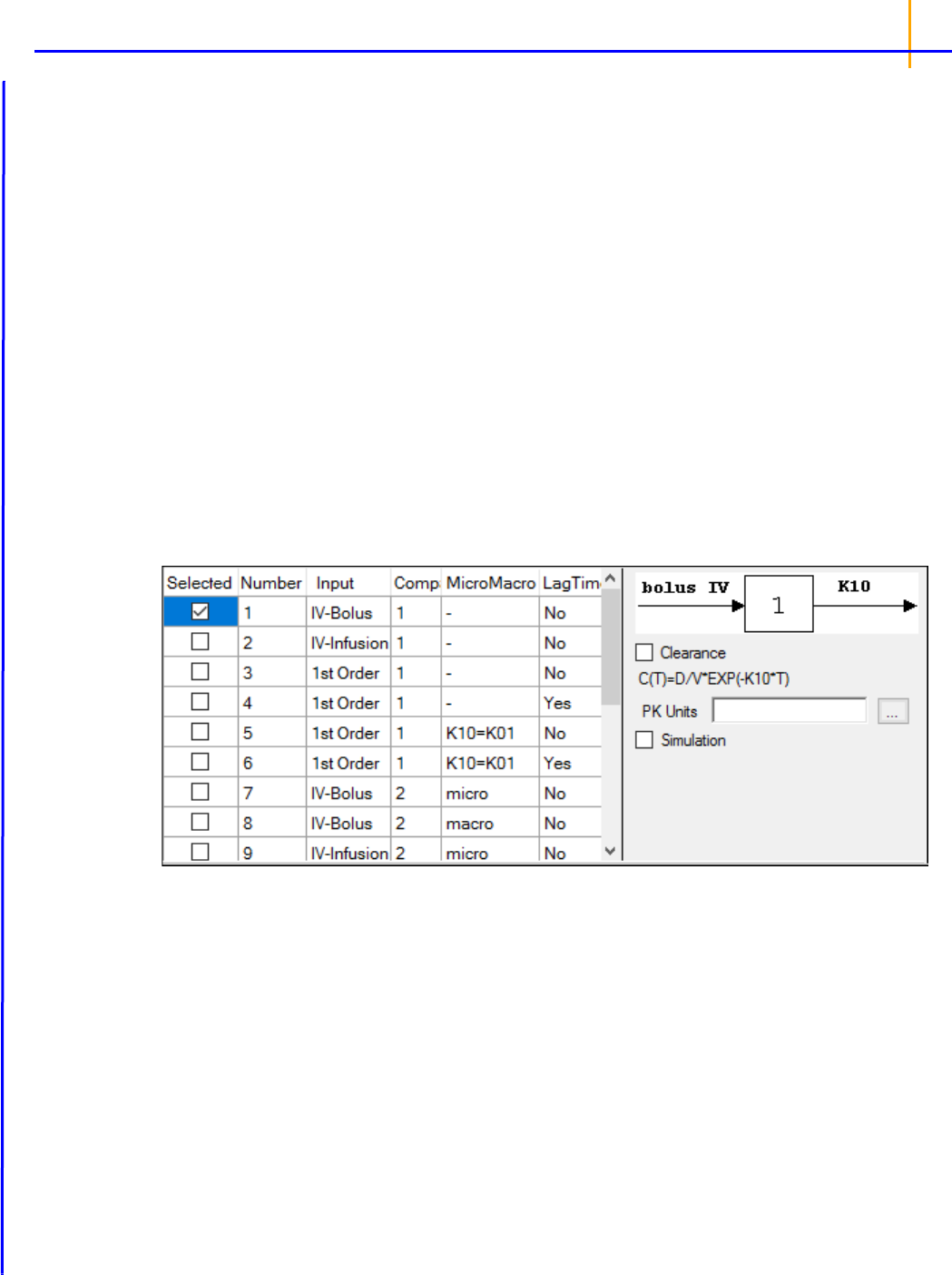
Least-Squares Regression Models interface

209

Format panel

The Format panel is only available for ASCII Models and is used to map ASCII code to an ASCII

model. Users can view and edit ASCII model code in this panel.

•Check the Use internal Text Object checkbox to edit the ASCII code. 



Phoenix displays a message box asking users if they want to copy the ASCII code to an internal

source:

• Click Yes to have the ASCII code copied to the internal text editor.

• Click No to remove the ASCII code and start with a blank internal text editor.

If ASCII code was previously mapped to the User ASCII Model panel then that code is displayed in

the internal text editor, instead of a blank panel.

More information on the text editor is available on the Syncfusion website.

Model Selection tab

The Model Selection tab for most of the Least-Squares Regression Models allows users to select a

model and whether or not the model uses simulated data/clearance parameter. (For the User ASCII

Model, the Model Selection tab contains weighting options as described in the

“Weighting/Dosing

Options tab”

description.)

• Check the checkbox beside the model number to choose it. For Dissolution models, click an

option button to select a model.

Refer to any of the following sections for model details:

Linear models

Michaelis-Menten models

Pharmacodynamic models

Pharmacokinetic models

Selecting a model displays a diagram beside the model selection menu that describes the

model’s functions. The model’s equation is listed beneath the diagram.

Phoenix WinNonlin

User’s Guide

210

• Set the options for the selected model.

• For Indirect Response, PK, and PK/PD Linked models, select the Clearance checkbox to

add a clearance parameter to the model. (The clearance parameter option is not available for

PK models 8, 10, 13, 14, 17, 18, or 19.)

• For Michaelis-Menten Models, use the Number of Constants box to type or select the num-

ber of dosing constants used per profile. (For more on how the number of constants corre-

sponds to the number, amount, and time of doses, see

“Dosing constants for the Michaelis-

Menten model”

• For PK/PD Linked Models, enter concentration units in the PK Units text field or click the

Units Builder […] button to use the Units Builder dialog.

Note: For PK/PD Linked Models, to view all PK parameter units in the PK Parameters panel, users must

supply concentration units in the PK Units text field in the Model Selection tab and dose units in

the Weighting/Dosing Options tab.

•Check the Simulation checkbox to simulate concentration data. Enter units for the simulated

data in the Y Units text field or click the Units Builder […] button to use the Units Builder dialog.



If the Simulation checkbox is selected then no concentration variable is required to run the

model.

Linked Model tab

The Linked Model tab allows users to select the model to link with model specified in the Model Selec-

tion tab. It is available only for the Indirect Response and PK/PD Linked Models.

Least-Squares Regression Models interface

211

• Check the checkbox beside the model number to choose it.

For more on these models, see

“Indirect Response models”. For PK/PD Linked Models, see “Pharma-

codynamic models”

For a list of PD output parameters used in linked PK/PD models, see

“PD output parameters in a PK/

PD model”

Selecting a model displays a diagram beside the model selection menu that describes the model’s

functions. The model’s equation is listed beneath the diagram.

Weighting/Dosing Options tab

The Weighting Options tab (in Dissolution, Linear, M-M, and PD Model objects) and the Weighting/

Dosing Options tab (in Indirect Response, PK, and PK/PD Linked Model objects) allows users to

select a weighting scheme and specify and preview dosing options.

Weighting options

• Use the Weighting menu to select one of six weighting schemes:

User Defined: Weights are read from a column in the dataset.

Uniform: Users can enter custom observed to or predicted to the power of N values. If selected,

then users must select Observed or Predicted in the Source menu and type the power value in

the Power to text field.

1/Y: Weight the data by 1/observed Y.

1/Yhat: Weight the data by 1/predicted Y (iterative reweighting).

1/(Y*Y): Weight the data by 1/observed Y

.

1/(Yhat*Yhat): Weight the data by 1/predicted Y

(iterative reweighting).

Phoenix WinNonlin

User’s Guide

212

• Use the Source menu to select one of three weighting sources:

Source: Selecting this option sets the weighting to User Defined and adds a Weight column to

the Main Mappings panel. If selected, users must map the weighting column in the dataset to the

Weight context in the Main Mappings panel.

Observed: Select to use weighted least squares. This is the default selection for 1/Y and 1/(Y*Y).

The default power for 1/Y is –1 and for 1/(Y*Y) it is –2.

Predicted: Select to use iterative reweighting. This is the default selection for 1/Yhat and 1/

(Yhat*Yhat). The default power for 1/Yhat is –1 and for 1/(Yhat*Yhat) it is –2.

• Type a power value in the Power to text field. (This option is disabled if Source is set to Source.)

Entering

-1 automatically sets the weighting to 1/Y (if Observed is the source) or 1/Yhat (if Pre-

dicted is the source).

Entering

-2 automatically sets the weighting to 1/(Y*Y) (if Observed is the source) or 1/

(Yhat*Yhat) (if Predicted is the source).

•Check the No Scaling checkbox to not scale the weighting for observed weighting values.



When weights are contained in a dataset or Observed is selected as the source, the weights for

individual data values are scaled so that the sum of weights for each function is equal to the num-

ber of data values. Weights must not be 0 (zero) in order to scale.



Scaling has no effect on the model fitting, because the weights of the observations are propor-

tionally the same. However, scaling weights provides increased numerical stability.

Dosing options

Available for Indirect Response, PK, and PK/PD Linked models.

• Enter the dosing unit in the Unit text field or click the […] button to use the Units Builder dialog to

set the dosing unit.

Note: For Indirect Response Models, to view all PK parameter units in the PK Parameters panel, users

must supply units for the time and concentration data in the input and specifying dose units in the

Weighting/Dosing Options tab.



For PK/PD Linked Models, to view all PK parameter units in the PK Parameters panel, users must

supply concentration units in the PK Units text field in the Model Selection tab and dose units in

the Weighting/Dosing Options tab.

• Use the Normalization menu to select the appropriate factor, if the dose amount is normalized by

subject body weight or body mass index. Options include: None, kg, g, mg, m**2, 1.73 m**2.



Dose normalization usage:

• If doses are in milligrams per kilogram of body weight, select mg as the dosing unit and kg as

the dose normalization.

•The Normalization menu affects the output parameter units. For example, if dose volume is

in liters, selecting kg as the dose normalization changes the units to

L/kg.

• Dose normalization affects units for all volume and clearance parameters in PK models.

• Type the number of doses per profile into the # Doses text field. (Only enabled if an internal work-

sheet is used for Dosing.) 

Least-Squares Regression Models interface

213



If different profiles require different numbers of doses, enter the highest number of doses.

• Click Preview Dosing to view a preview of dose option selections. 



If an external dosing data worksheet is used to provide dosing data, then the preview window will

show the number of doses and dosing time points per profile. Click OK to close the preview win-

dow.

Parameter Options tab

All iterative estimation procedures require initial estimates of the parameter values. Phoenix com-

putes initial estimates via curve stripping for single-dose models. For all other situations, including

multiple-dose models, users must provide initial estimates or boundaries to be used by Phoenix in

creating initial estimates. Parameter boundaries provide a basis for grid searching initial parameter

estimates, and also limit the estimates during modeling. This is useful if the values become unrealistic

or the model does not converge. For more on setting initial parameter estimates, refer to

“Parameter

Estimates and Boundaries Rules”

Set the parameter calculation method:

Note: The default minimization method, Gauss-Newton (Hartley) (located in the Engine Settings tab),

and the Parameter Boundaries option Do Not Use Bounds are recommended for all Linear mod-

els.

• Select the User Supplied Initial Parameter Values option button to enter initial parameter esti-

mates in the Initial Estimates panel.

Or

Select the WinNonlin Generated Initial Parameter Values option button to have Phoenix deter-

mine the initial parameter values.

• If the User Supplied Bounds option button is selected, Phoenix uses curve stripping to pro-

vide initial estimates. If curve stripping fails, then Phoenix uses the grid search method.

• If the WinNonlin Bounds option button is selected, Phoenix uses curve stripping to provide

initial estimates, and then applies boundaries to the model parameters for model fitting. If

curve stripping fails, the model fails because Phoenix cannot use grid search for initial esti-

mates without user-supplied boundaries.

•Check the Propagate Final Estimates checkbox to propagate initial parameter estimates across

all sort levels.

This option is available when more than one sort variable is used in the main dataset.



If this option is selected, then initial estimates and boundaries are entered or mapped only for the

first sort level. The final parameter estimates from the first sort level provide the initial estimates

for each consecutive sort level.

Set the boundary calculation method:

Parameter boundaries provide a basis for grid searching initial parameter estimates, and also limit the

estimates during modeling. This is useful if the values become unrealistic or the model does not con-

F

P 1

--------------

FP1 +FP1–



---------------------------------------------------------

Phoenix WinNonlin

User’s Guide

214

verge. For more on using parameter boundaries, refer to “Parameter Estimates and Boundaries

Rules”.

•

Select the User Supplied Initial Bounds option to enter parameter boundaries in the Initial Esti-

mates panel.

Or select the WinNonlin Bounds option to have Phoenix determine the parameter boundaries.

Or select the Do No Use Bounds option to not use parameter boundaries.

Engine Settings tab

The Engine Settings tab provides control over the model fitting algorithm and related settings.

• Use the Minimization menu to select the method to use with the Indirect Response model.



Method 1: The Nelder-Mead algorithm does not require the estimated variance-covariance

matrix as part of its algorithm, so it often performs very well on ill-conditioned datasets. Ill-condi-

tioned indicates that, for the given dataset and model, there is not enough information contained

in the data to precisely estimate all of the parameters in the model or that the sum of squares sur-

face is highly curved. Although the procedure works well, it can be slow, particularly when used to

fit a system of differential equations.



Method 2: Gauss-Newton (Levenberg and Hartley) is the default algorithm and performs well

on a wide class of problems, including ill-conditioned datasets. Although the Gauss-Newton

method does require the estimated variance-covariance matrix of the parameters, the Levenberg

modification suppresses the magnitude of the change in parameter values from iteration to itera-

tion to a reasonable amount. This enables the method to perform well on ill-conditioned datasets.



Method 3: Gauss-Newton (Hartley) is another Gauss-Newton method. It is not as robust as

Methods 1 and 2 but is extremely fast. Method 3 is recommended when speed is a consideration

or when maximum likelihood estimation or linear regression analysis is to be performed. It is not

recommended for fitting complex models.

Note: The use of bounds is recommended with Methods 2 and 3. For linear regressions, use Method 3

without bounds.

•In the Increment for Partial Derivatives text field, type the incremental value that the parameter

value is to be multiplied by.



Nonlinear algorithms require derivatives of the models with respect to the parameters. The pro-

gram estimates these derivatives using a difference equation. For example (

= the increment

with which the parameter value is multiplied)

• In the Number of Predicted Values text field, type the number of predicted values used to deter-

mine the number of points in the predicted data.

Least-Squares Regression Models Results

215



Use this option to create a dataset that will plot a smooth curve. When fitting or simulating multiple

dose data, the predicted data plots may be much improved by increasing the number of predicted

values. The minimum allowable value is 10; the maximum is 20,000.



If the number of derivatives is greater than zero (i.e., differential equations are used), this com-

mand is ignored and the number of predicted points is equal to the number of points in the data-

set.



For compiled models without differential equation, the default value is 1000. The default for user

models is the number of data points in the original dataset. This value may be increased only if

the model has no more than one independent variable.

Note: To better reflect peaks (for IV dosing) and troughs (for extravascular, IV infusion and IV bolus dos-

ing), the predicted data for the built-in PK models includes dosing times, in addition to the concen-

trations generated. For all three types, concentrations are generated at dosing times; in addition,

for infusion models, data are generated for the end of infusion.

• In the Convergence Criteria text field, type the criterion value used to determine convergence. 



The default is 0.0001. Convergence is achieved when the relative change in the residual sum of

squares is less than the convergence criterion.

• Leave the Meansquare text field blank, unless the mean square needs to be a fixed value in

order to compute the variance in a model.



The variance is normally a function of the weighted residual SS/df, or the Mean Square. For cer-

tain types of problems, when computing the variance, the mean square needs to be set to a fixed

value.

• Leave the Iterations text field set to its default value, unless the purpose of the model is to evalu-

ate it, and not fit it. 



The default iteration values are:

500 for Nelder-Mead minimization. Each iteration is a reflection of the simplex.

50 for Gauss-Newton (Levenberg and Hartley) or Gauss-Newton (Hartley) minimizations.

• Type a value of

0 (zero) in the Iterations text field if the purpose of the model is evaluation. 



A value of

0 requires users to supply their own initial parameter values and all output will use the

initial estimates as the final parameters.

Least-Squares Regression Models Results

Note: This section is meant to provide guidance and references to aid in the interpretation of modeling

output, and is not a replacement for a PK or statistics textbook.

After a Classic model is run, the output is displayed on the Results tab in Phoenix. The output is dis-

cussed in the following sections.

Core Output: text version of all model settings and output, including any errors that occurred

during modeling. See

“Core Output File” for a full description.

Settings: test version of all user-defined settings.

Phoenix WinNonlin

User’s Guide

216

Worksheet output: worksheets listing input data, modeling iterations and output parameters, as

well as several measures of fit.

Plot output: plots of observed and predicted data, residuals, and other quantities, depending on

the model run.

Worksheet output

Worksheet output contains summary tables of the modeling data and a summary of the information in

the Core Output. The worksheets generated depend on the analysis type and model settings. They

present the output in a form that can be used for reporting and further analyses and are listed on the

Results tab underneath Output Data.

Condition Numbers: Rank and condition number of the matrix of partial derivatives for each itera-

tion. 

The matrix is of full rank, since Rank is equal to the number of parameters. If the Rank were less than

three, that would indicate that there was not enough information in the data to estimate all three

parameters. The condition value is the square root of the ratio of the largest to the smallest eigen-

value and values should be less than 10^n where n is the number of parameters.

Correlation Matrix: A correlation matrix for the parameters, for each sort level. If any values get

close to 1 or –1, there may be too many parameters in the model and a simpler model may work bet-

ter.

Diagnostics: Diagnostics for each function in the model and for the total:

CSS: corrected sum of squared observations 

WCSS: weighted corrected sum of squared observations 

SSR: sum of squared residuals 

WSSR: weighted sum of squared residuals 

S: estimate of residual standard deviation 

DF: degrees of freedom 

CORR_(OBS,PRED): correlation between observed Y and predicted Y 

WT_CORR_(OBS,PRED): weighted correlation 

AIC: Akaike Information Criterion goodness of fit measurement 

SBC: Schwarz Bayesian Criterion goodness of fit measurement

Differential Equations: The value of the partial derivatives for each parameter at each time point for

each value of the sort variables.

Dosing Used: The dosing regimen specified for the modeling.

Eigenvalues: Eigenvalues for each level of the sort variables. (An eigenvalue of matrix A is a number

, such that Ax=x for some vector x, where x is the eigenvector. Eigenvalues and their associated

eigenvectors can be thought of as building blocks for matrices.)

Final Parameters and Final Parameters Pivoted: Parameter names, units, estimates, standard

error of the estimates, CV% (values < 20% are generally considered to be very good), univariate

intervals, and planar intervals for each level of the sort variables.

Fitted Values: (Dissolution models) Predicted data for each profile.

Initial Estimates: Parameter names, initial values, and lower and upper bounds for each level of the

sort variables.

Minimization Process: Iteration number, weighted sum of squares, and value for each parameter,

for each level of the sort variables. This worksheet shows how parameter values converged as the

iterations were performed. If the number of iterations is approaching the specified limit, there may be

some problems with the model.

Least-Squares Regression Models Results

217

Parameters: (Dissolution models) The smoothing parameter delta and absorption lag time for each

profile.

Partial Derivatives and Stacked Partial Derivatives: Values of the differential equations at each

time in the dataset.

Predicted Data: Time and predicted Y for multiple time points, for each sort level.

Secondary Parameters and Secondary Parameters Pivoted: Available for Michaelis-Menten, PK,

PD, PK/PD Linked and ASCII models. Secondary parameter name, units, estimate, standard error of

the estimate, and CV% for each sort level.

Summary Table

: The sort variables, X, Y, transformed X, transformed Y, predicted Y, residual,

weight, standard error of predicted Y, standardized residuals, for each sort level. For link models, also

includes C

and C

. For indirect response models, also includes C

Values: (Dissolution models) Time, input rate, cumulative amount (Cumul_Amt, using the dose units)

and fraction input (Cumul_Amt/test dose or, if no test doses are given, then fraction input approaches

one) for each profile.

Variance Covariance Matrix: A variance-covariance matrix for the parameters, for each sort level.

User Settings: Model number, minimization method, convergence criterion, maximum number of iter-

ations allowed, and the weighting scheme.

AIC and SBC are only meaningful during comparison of models. A smaller value is better, negative is

better than positive, and a more negative value is even better. AIC is computed as:

AIC=

N log (WRSS)+2P, where N is the number of observations with positive weight, log is the natural

logarithm,

WRSS is the weighted residual sum of squares, P is the number of parameters.

If there are no statements to transform the data, then X and Y will equal X(obs) and Y(obs).

Plot output

Analysis produces up to eight graphs that are divided by each level of the sort variable. Plot output is

listed underneath Plots in the Results tab.

Cumulative Rates: (Dissolution models) Cumulative drug input vs. time.

Fitted Curves: (Dissolution models) Observed time-concentration data vs. the predicted curve.

Input Rates: (Dissolution models) Rate of drug input vs. time.

Observed Y and Predicted Y vs X: plots the predicted curves as a function of X, with the Observed

Y overlaid on the plot. Used for assessing the model fit.

Partial Derivatives Plot: plots the partial derivative of the model with respect to each parameter as a

function of the

x variable. If f(x; a, b, c) is the model as a function of x, based on parameters a, b, and

c, then df(x; a, b, c)/da, df(x; a, b, c)/db, df(x; a, b, c)/dc are plotted versus x. Each derivative is

evaluated at the final parameter estimates. Data taken at larger partial derivatives are more influential

than those taken at smaller partial derivatives for the parameter of interest.

Predicted Y vs Observed Y: plots weighted Y against observed Y. Scatter should lie close to the 45

degree line.

Residual Y vs Predicted Y: used to assess whether error distribution is appropriately modeled

throughout the range of the data.

Residual Y vs X: used to assess whether error distribution is appropriately modeled across the range

of the X variable.

Phoenix WinNonlin

User’s Guide

218

• Weighted Predicted Y vs Observed Y: plots weighted predicted Y against observed Y. Scatter

should lie close to the 45 degree line; only produced if a non-Uniform weighting scheme is used.

• Weighted Residual Y vs Observed Y: used to assess whether error distribution is appropriately

modeled across the range of the observed Y variable; only produced if a non-Uniform weighting

scheme is used.

• Weighted Residual Y vs Predicted Y: used to assess whether error distribution is appropriately

modeled across the range of the predicted variable; only produced if a non-Uniform weighting

scheme is used.

• Weighted Residual Y vs Weighted Predicted Y: used to assess whether error distribution is

appropriately modeled throughout the range of the data; only produced if a non-Uniform weight-

ing scheme is used.

• Weighted Residual Y vs X: used to assess whether error distribution is appropriately modeled

across the range of the X variable; only produced if a non-Uniform weighting scheme is used.

Users can double-click any plot in the Results tab to edit it. (See the

“Plot Options tab” description for

editing options.)

Nonlinear Regression Overview

219

Nonlinear Regression Overview

YABX++=

++ + +=

++++=

BX–exp=

max

C+

------------------

X–exp A

X–exp+=

Modeling and nonlinear regression

Model fitting algorithms and features of Phoenix WinNonlin

Modeling and nonlinear regression

The value of mathematical models is well recognized in all of the sciences — physical, biological,

behavioral, and others. Models are used in the quantitative analysis of all types of observations or

data, and with the power and availability of computers, mathematical models provide convenient and

powerful ways of looking at data. Models can be used to help interpret data, to test hypotheses, and to

predict future results. The main concern here is with “fitting” models to data — that is, finding a math-

ematical equation and a set of parameter values such that values predicted by the model are in some

sense “close” to the observed values.

Most scientists have been exposed to linear models, models in which the dependent variable can be

expressed as the sum of products of the independent variables and parameters. The simplest exam-

ple is the equation of a line (simple linear regression):

where

Y is the dependent variable, X is the independent variable, A is the intercept and B is the

slope. Two other common examples are polynomials such as:

and multiple line

ar regression.

These examples are all “linear mod

els” since the parameters appear only as coefficients of the inde-

pendent variables.

In nonlinear models, at least one of the parameters appears as other than a coefficient. A simple

example is the decay curve:

This model can be linearized by ta

king the logarithm of both sides, but as written it is nonlinear.

Another example is the Michaelis-Menten equation:

This example can also be lin

earized by writing it in terms of the inverses of V and C, but better esti-

mates are obtained if the nonlinear form is used to model the observations (Endrenyi, ed. (1981),

pages 304–305).

There are many models which cannot be made linear by transformation. One such model is the sum

of two or more exponentials, such as:

Phoenix WinNonlin

User’s Guide

220

All of the models on this page are called nonlinear models, or nonlinear regression models. Two good

references for the topic of general nonlinear modeling are Draper and Smith (1981) and Beck and

Arnold (1977). The books by Bard (1974), Ratkowsky (1983) and Bates and Watts (1988) give a more

detailed discussion of the theory of nonlinear regression modeling. Modeling in the context of kinetic

analysis and pharmacokinetics is discussed in Endrenyi, ed. (1981) and Gabrielsson and Weiner

(2016).

All pharmacokinetic models derive from a set of basic differential equations. When the basic differen-

tial equations can be integrated to algebraic equations, it is most efficient to fit the data to the inte-

grated equations. But it is also possible to fit data to the differential equations by numerical

integration. Phoenix WinNonlin can be used to fit models defined in terms of algebraic equations and

models defined in terms of differential equations as well as a combination of the two types of equa-

tions.

Given a model of the data, and a set of data, how is the model “fit” to the data? Some criterion of “best

fit” is needed, and many have been suggested, but only two are much used. These are maximum

likelihood and least squares. With certain assumptions about the error structure of the data (no ran-

dom effects), the two are equivalent. A discussion of using nonlinear least squares to obtain maxi-

mum likelihood estimates can be found in Jennrich and Moore (1975). In least squares fitting, the

“best” estimates are those which minimize the sum of the squared deviations between the observed

values and the values predicted by the model.

The sum of squared deviations can be written in terms of the observations and the model. In the case

of linear models, it is easy to compute the least squares estimates. One equates to zero the partial

derivatives of the sum of squares with respect to the parameters. This gives a set of linear equations

with the estimates as unknowns; well-known techniques can be used to solve these linear equations

for the parameter estimates.

This method will not work for nonlinear models, because the system of equations which results by

setting the partial derivatives to zero is a system of nonlinear equations for which there are no general

methods for solving. Consequently, any method for computing the least squares estimates in a non-

linear model must be an iterative procedure. That is, initial estimates of the parameters are made and

then, in some way, these initial estimates are modified to give better estimates, i.e., estimates which

result in a smaller sum of squared deviations. The iteration continues until hopefully the minimum (or

least) sum of squares is reached.

In the case of models with random effects, such as population PK/PD models, the more general

method of maximum likelihood (ML) must be employed. In ML, the likelihood of the data is maximized

with respect to the model parameters. The LinMix operational object fits models of this variety.

Since it is not possible to know exactly what the minimum is, some stopping rule must be given at

which point it is assumed that the method has converged to the minimum sum of squares. A more

complete discussion of the theory underlying nonlinear regression can be found in the books cited

previously.

Model fitting algorithms and features of Phoenix WinNonlin

Phoenix WinNonlin estimates the parameters in a nonlinear model, using the information contained in

a set of observations. Phoenix WinNonlin can also be used to simulate a model. That is, given a set of

parameter values and a set of values of the independent variables in the model, Phoenix WinNonlin

will compute values of the dependent variable and also estimate the variance-inflation factors for the

estimated parameters.

A computer program such as Phoenix WinNonlin is only an aid or tool for the modeling process. As

such it can only take the data and model supplied by the researcher and find a “best fit” of the model

to the data. The program cannot determine the correctness of the model nor the value of any deci-

Nonlinear Regression Overview

221

sions or interpretations based on the model. The program does, however, provide some information

about the “goodness of fit” of the model to the data and about how well the parameters are estimated.

It is assumed that the user of Phoenix WinNonlin has some knowledge of nonlinear regression such

as contained in the references mentioned earlier. Phoenix WinNonlin provides the “least squares”

estimates of the model parameters as discussed above. The program offers three algorithms for min-

imizing the sum of squared residuals: the simplex algorithm of Nelder and Mead (1965), the Gauss-

Newton algorithm with the modification proposed by Hartley (1961), and a Levenberg-type modifica-

tion of the Gauss-Newton algorithm (Davies and Whitting (1972)).

The simplex algorithm is a very powerful minimization routine; its usefulness has formerly been lim-

ited by the extensive amount of computation it requires. The power and speed of current computers

make it a more attractive choice, especially for those problems where some of the parameters may

not be well-defined by the data and the sum of squares surface is complicated in the region of the

minimum. The simplex method does not require the solution of a set of equations in its search and

does not use any knowledge of the curvature of the sum of squares surface. When the Nelder-Mead

algorithm converges, Phoenix WinNonlin restarts the algorithm using the current estimates of the

parameters as a “new” set of initial estimates and ting the step sizes to their original values. The

parameter estimates which are obtained after the algorithm converges a second time are treated as

the “final” estimates. This modification helps the algorithm locate the global minimum (as opposed to

a local minimum) of the residual sum of squares for certain difficult estimation problems.

The Gauss-Newton algorithm uses a linear approximation to the model. As such it must solve a set of

linear equations at each iteration. Much of the difficulty with this algorithm arises from singular or

near-singular equations at some points in the parameter space.Phoenix WinNonlin avoids this diffi-

culty by using singular value decomposition rather than matrix inversion to solve the system of linear

equations. (See Kennedy and Gentle (1980).) One result of using this method is that the iterations do

not get “hung up” at a singular point in the parameter space, but rather move on to points where the

problem may be better defined. To speed convergence, Phoenix WinNonlin uses the modification to

the Gauss-Newton method proposed by Hartley (1961) and others; with the additional requirement

that at every iteration the sum of squares must decrease.

Many nonlinear estimation programs have found Hartley’s modification to be very useful. Beck and

Arnold (1977) compare various least squares algorithms and conclude that the Box-Kanemasu

method (almost identical to Hartley’s) is the best under many circumstances.

As indicated, the singular value decomposition algorithm will always find a solution to the system of

linear equations. However, if the data contain very little information about one or more of the parame-

ters, the adjusted parameter vector may be so far from the least squares solution that the linearization

of the model is no longer valid. Then the minimization algorithm may fail due to any number of numer-

ical problems. One way to avoid this is by using a ‘trust region’ solution; that is, a solution to the sys-

tem of linear equations is not accepted unless it is sufficiently close to the parameter values at the

current iteration. The Levenberg and Marquardt algorithms are examples of ‘trust region’ methods.

Note: The Gauss-Newton method with the Levenberg modification is the default estimation method used

by Phoenix WinNonlin.

Trust region methods tend to be very robust against ill-conditioned data sets. There are two reasons,

however, why one may not want to use them. (1) They require more computation, and thus are not

efficient with data sets and models that readily permit precise estimation of the parameters. (2) More

importantly, the trust region methods obtain parameter estimates that are often meaningless because

of their large variances. Although Phoenix WinNonlin gives indications of this, it is possible for users

to ignore this information and use the estimates as though they were really valid. For more informa-

tion on trust region methods, see Gill, Murray and Wright (1981) or Davies and Whitting (1972).

Phoenix WinNonlin

User’s Guide

222

In Phoenix WinNonlin, the partial derivatives required by the Gauss-Newton algorithm are approxi-

mated by difference equations. There is little, if any, evidence that any nonlinear estimation problem is

better or more easily solved by the use of the exact partial derivatives.

To fit those models that are defined by systems of differential equations, the RKF45 numerical inte-

gration algorithm is used (Shampine, Watts and Davenport (1976)). This algorithm is a 5th order

Runge-Kutta method with variable step sizes. It is often desirable to set limits on the admissible

parameter space; this results in “constrained optimization.” For example, the model may contain a

parameter which must be non-negative, but the data set may contain so much error that the actual

least squares estimate is negative. In such a case, it may be preferable to give up some of the prop-

erties of the unconstrained estimation in order to obtain parameter estimates that are physically real-

istic. At other times, setting reasonable limits on the parameter may prevent the algorithm from

wandering off and getting lost. For this reason, it is recommend that users always set limits on the

parameters (the means of doing this is discussed in

“Parameter Estimates and Boundaries Rules”

and

“Modeling”). In Phoenix WinNonlin, two different methods are used for bounding the parameter

space. When the simplex method is used, points outside the bounds are assigned a very large value

for the residual sum of squares. This sends the algorithm back into the admissible parameter space.

With the Gauss-Newton algorithms, two successive transformations are used to affect the bounding

of the parameter space. The first transformation is from the bounded space as defined by the input

limits to the unit hypercube. The second transformation uses the inverse of the normal probability

function to go to an infinite parameter space. This method of bounding the parameter space has

worked extremely well with a large variety of models and data sets.

Bounding the parameter space in this way is, in effect, a transformation of the parameter space. It is

well known that a reparameterization of the parameters will often make a problem more tractable.

(See Draper and Smith (1981) or Ratkowsky (1983) for discussions of reparameterization.) When

encountering a difficult estimation problem, the user may want to try different bounds to see if the esti-

mation is improved. It must be pointed out that it may be possible to make the problem worse with this

kind of transformation of the parameter space. However, experience suggests that this will rarely

occur. Reparameterization to make the models more linear also may help.

Because of the flexibility and generality of Phoenix WinNonlin, and the complexity of nonlinear esti-

mation, a great many options and specifications may be supplied to the program. In an attempt to

make Phoenix WinNonlin easy to use, many of the most commonly used options have been internally

specified as defaults.

Phoenix WinNonlin is capable of estimating the parameters in a very large class of nonlinear models.

Fitting pharmacokinetic and pharmacodynamic models is a special case of nonlinear estimation, but it

is important enough that Phoenix WinNonlin is supplied with a library of the most commonly used

pharmacokinetic and pharmacodynamic models. To speed execution time, the main Phoenix Win-

Nonlin library has been built-in, or compiled. However, ASCII library files corresponding to the same

models as the built-in models, plus an additional utility library of models, are also provided.

Least-Squares Regression Model calculations

223

Least-Squares Regression Model calculations

Indirect Response models

Linear models

Michaelis-Menten models

Pharmacodynamic models

Pharmacokinetic models

PD output parameters in a PK/PD model

ASCII Model dosing constants

Parameter Estimates and Boundaries Rules

References

Indirect Response models

When the pharmacologic response takes time to develop and the observed response is not directly

related to plasma concentrations of the drug a link model can be applied to relate the pharmacokinet-

ics of the drug to its pharmacodynamics. Phoenix contains a group of indirect pharmacodynamic

response (IPR) models proposed by Jusko (1990) and Dayneka, Garg, and Jusko (1993). The indi-

rect response models differ from other models in Phoenix in that they use a PK model to predict con-

centrations, and then use these concentrations as input to the indirect PD response model.

Model 51: Inhibition of input.

Estimated parameters: Kin Kout IC

Model 52: Inhibition of output.

Estimated parameters: Kin Kout IC

Model 53: Stimulation of input.

------

------------------------

–







out

R–=

------

out

------------------------

–







– R=

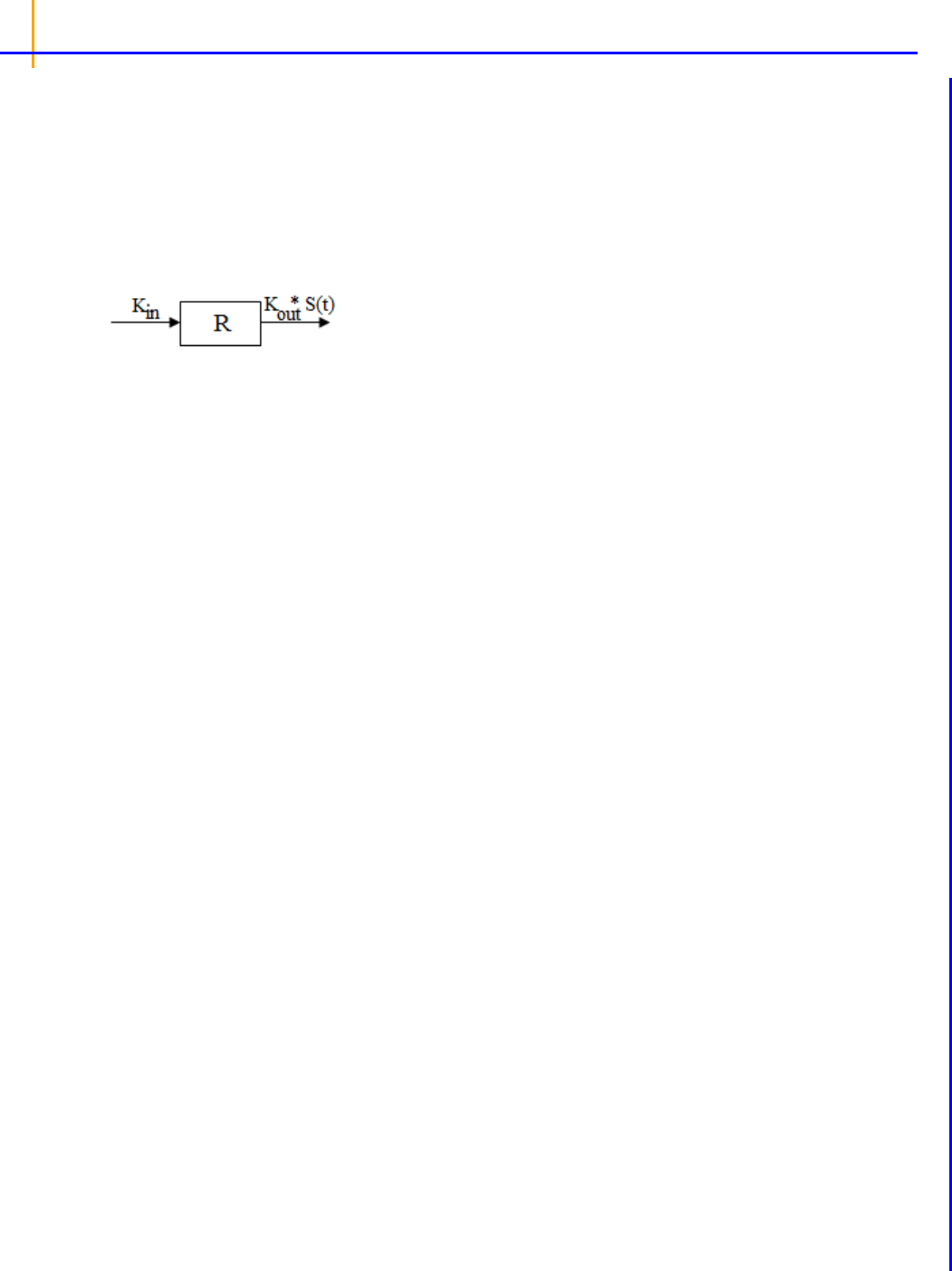
Phoenix WinNonlin

User’s Guide

224

Estimated parameters: Kin Kout EC

Emax

Model 54: Stimulation of output.

Estimated parameters: Kin Kout EC

Emax

Model notation

R: Measured response to a drug.

: The zero-order constant for the production of response.

out

: The first-order rate constant for loss of response.

Cp: Plasma concentration of a drug.

Ce: Drug concentration at the effect site.

: Drug concentration required to produce 50% of the maximal inhibition.

Emax: Maximum drug effect.

: Concentration in plasma that achieves 50% of predicted maximum effect in an Emax model.

------

Emax C

--------------------------







out

R–=

------

out

Emax C

--------------------------







– R=

225

Linear models

Phoenix contains four Linear models used to perform linear regression. In the following table the y-

unit is the preferred unit of the

y (concentration) variable and the t-unit is the preferred unit of the t

(time) variable. See

“Units panel” to set preferred units for the output parameters.

The linear models do not require dosing information.

Note: The default minimization method, Gauss-Newton (Hartley) (located in the Engine Settings tab),

and the Parameter Boundaries option Do Not Use Bounds are recommended for all linear mod-

els.

Linear models include:



y(t)=CONSTANT



Estimated Parameters: CONSTANT (y-unit)



y(t)=INT+SLOPE*t



Estimated Parameters: INT (y-unit), SLOPE (y-unit/t-unit)



y(t)=A0+A1*t+A2*t



Estimated Parameters:

A0 (y-unit), A1 (y-unit/t-unit), A2 (y-unit/t-unit

)



y(t)=A0+A1*t+A2*t

+A3*t



Estimated Parameters:

A0 (y-unit), A1 (y-unit/t-unit), A2 (y-unit/t-unit

), A3 (y-unit/t-unit

)

Phoenix WinNonlin

User’s Guide

226

Michaelis-Menten models

The Michaelis-Menten models describe the relationship between the rate of substrate conversion by

an enzyme to the concentration of the substrate. These kinetics are valid only when the concentration

of substrate is higher than the concentration of enzyme, and in the case of steady-state, where the

concentration of the complex enzyme-substrate is constant.

The Phoenix library contains four Michaelis-Menten models that use constants to supply the dosing

information. The required number of constants are listed below under each model number. For an

explanation of dosing constants see

“Dosing constants for the Michaelis-Menten model”.

Phoenix assumes that the time of the first dose is zero. For these models, times in the dataset must

correspond to the dosing times, even if these times contain no observations. In this case, include a

column for Weight in the dataset, and weight the observations as zero.

These models parameterize

Vmax in terms of concentration per unit of time.

For a discussion of the difficulties in fitting the Michaelis-Menten models see Tong and Metzler (1980)

and Metzler and Tong (1981).

Model 301

One-compartment with bolus input and Michaelis-Menten output.



C(t) is the solution to the differential equation:

with initial condition

C(0)=D/V.

Required constants: Number of doses (N), Dose amount for dose N, Time of dose for dose N

Estimated parameters: V is the volume, Vmax is the max elimination rate, Km is the Michaelis con-

stant

Secondary parameters: AUC=(D/V)(D/V/2+Km)/ Vmax

Model 302

One-compartment with constant IV input and Michaelis-Menten output.



C(t) is the solution to the differential equations:

-------

Vmax C

Km C+

-----------------------

–=

-------

tinf V

-----------------

Vmax C

Km C+

-----------------------

for tTinf

-------

–

Vmax C

Km C+

-----------------------

– for tTinf

227

with initial condition C(0)=0.

Required constants: Number of doses (N), Dose amount for dose N, Start time of dose for dose N,

End time for dose N

Estimated parameters: V is the volume, Vmax is the max elimination rate, Km is the Michaelis con-

stant

Secondary parameters: None

Model 303

One-compartment with first-order input, Michaelis-Menten output and no lag time.



C(t) is the solution to the differential equation:

with initial condition

C(0)=0.

Required constants: Number of doses (N), Dose amount for dose N, Time of dose for dose N

Estimated parameters: V_F, K01 is the absorption rate, Vmax is the max elimination rate, Km is the

Michaelis constant

Secondary parameters: K01 half-life

Model 304

One-compartment with first-order input, Michaelis-Menten output and lag time.



C(t) is the solution to the differential equation:

with initial condition

C(0)=0.

Required constants: Number of doses (N), Dose amount for dose N, Time of dose for dose N

Estimated parameters: V_F, K01 is the absorption rate, Vmax is the max elimination rate, Km is the

Michaelis constant, Tlag is the lag time

Secondary parameters: K01 half-life

-------

K01

----

K01 t–

Vmax C

Km C+

-----------------------

–exp=

-------

K01

----

K01 t–exp

Vmax C

Km C+

-----------------------

for tTlag

-------

–

Vmax C

Km C+

-----------------------

for ttlag–

Phoenix WinNonlin

User’s Guide

228

Dosing constants for the Michaelis-Menten model

The number of constants in the model corresponds to the dosing route for the model.

Bolus and first-order input models require at least three dosing constants per profile:

CON[0]: Number of doses (N)

CON[1]: Dose amount for dose N

CON[2]: Time of dose for dose N

CON[3]: Dose amount for dose N+1 (if multiple doses are used)

CON[4]: Time of dose for dose N+1 (if multiple doses are used)

Constant IV infusion models require at least four dosing constants per profile:

CON[0]: Number of doses (N)

CON[1]: Dose amount for dose N

CON[2]: Start time for dose N

CON[3]: End time for dose N

CON[4]: Dose amount for dose N+1 (if multiple doses are used)

CON[5]: Start time for dose N+1 (if multiple doses are used)

CON[6]: End time for dose N+1 (if multiple doses are used)

229

Pharmacodynamic models

When pharmacological effects are seen immediately and are directly related to the drug concentra-

tion, a pharmacodynamic model is applied to characterize the relationship between drug concentra-

tions and effect. Phoenix includes the following PD models:

Notation definitions

Emax: Maximum drug effect.

Imax: Maximum drug inhibition.

: Baseline effect (effect at C=0).

: Concentration in plasma that achieves 50% of predicted maximum effect in an Emax

model.

: Drug concentration required to produce 50% of the maximal inhibition.

Rmax: Effect at infinity (includes maximum drug effect/inhibition and baseline).

F_Emax: Fractional change in effect from baseline E



Gamma: Shape parameter

Model 101: Simple Emax model.



Estimated parameters: Emax, EC

Effect = 0 at C=0 and Emax at C=infinity

Model 102: Simple Emax model with a baseline effect parameter.



Estimated parameters: Emax, EC

, E

Secondary parameters: Rmax=Emax+E

, F_Emax=Emax/E

Effect = E0 at C=0 and Emax + E0 at C=infinity

Emax C

CEC

-----------------------

Emax C

CEC

-----------------------

Phoenix WinNonlin

User’s Guide

230

Model 103: Inhibitory effect model.



Estimated parameters: E

, IC

Effect = 0 at C=0 and Emax at C=infinity

Model 104: Inhibitory effect model with a baseline effect parameter.



Estimated parameters: Imax, IC

50,

Secondary parameters: Rmax=E

– Imax, F_Imax=Imax/E

Effect = E0 at C=0 and E0 – Imax at C=infinity

Model 105: Sigmoid Emax model.



Estimated parameters: Emax, EC

, Gamma

Effect = 0 at C=0 and Emax at C=infinity

CIC

----------------------

–





Imax C

CIC

----------------------

–=

Emax C







----------------------------

231

Model 106: Sigmoid Emax model with a baseline effect parameter.



Estimated parameters: Emax, EC

, E

, Gamma

Secondary parameters: Rmax=Emax+E

, F_Emax=Emax/E

Effect = E0 at C=0 and Emax + E0 at C=infinity

Model 107: Sigmoid inhibitory effect model.



Estimated parameters: E

, IC

, Gamma

Effect = E0 at C=0 and 0 at C=infinity

Model 108: Sigmoid inhibitory effect model with a baseline effect parameter.



Estimated parameters: Imax, IC

, E

, Gamma

Secondary parameters: Rmax=E

– Imax, F_Imax=Imax/E

Effect = E0 at C=0 and E0 – Imax at C=infinity

Emax C







----------------------------



--------------------------

–







Imax C







--------------------------

–=

Phoenix WinNonlin

User’s Guide

232

Pharmacokinetic models

Phoenix includes nineteen pharmacokinetic (PK) models. Each is available in the PK Model object.

Model 1: IV-bolus input, 1-compartment, no lag, 1st order elimination

Model 2: IV-infusion input, 1-compartment, no lag, 1st order elimination

Model 3 1st order input, 1-compartment, no lag, 1st order elimination

Model 4 1st order input, 1-compartment, yes lag, 1st order elimination

Model 5 1st order input, 1-compartment, K10=K01 parameterization, no lag, 1st order elimination

Model 6 1st order input, 1-compartment, K10=K01 parameterization, yes lag, 1st order elimination

Model 7 IV-bolus input, 2-compartment, micro parameterization, no lag, 1st order elimination

Model 8 IV-bolus input, 2-compartment, macro parameterization, no lag, 1st order elimination

Model 9 IV-infusion input, 2-compartment, micro parameterization, no lag, 1st order elimination

Model 10 IV-infusion input, 2-compartment, macro parameterization, no lag, 1st order elimination

Model 11 1st order input, 2-compartment, micro parameterization, no lag, 1st order elimination

Model 12 1st order input, 2-compartment, micro parameterization, yes lag, 1st order elimination

Model 13 1st order input, 2-compartment, macro parameterization, no lag, 1st order elimination

Model 14 1st order input, 2-compartment, macro parameterization, yes lag, 1st order elimination

Model 15 IV-bolus + IV-infusion input, 1-compartment, micro parameterization, no lag, 1st order elimi-

nation

Model 16 IV-bolus + IV-infusion input, 2-compartment, micro parameterization, no lag, 1st order elimi-

nation

Model 17 IV-bolus + IV-infusion input, 2-compartment, macro parameterization, no lag, 1st order elim-

ination

Model 18 IV-bolus input, 3-compartment, macro parameterization, no lag, 1st order elimination

Model 19 IV-infusion input, 3-compartment, macro parameterization, no lag, 1st order elimination

Note: All models except models 15–17 accept multiple dose data.

The models shown in this section give equations for compartment 1 (central).

Model 1

One-compartment with IV-bolus input and first-order output.

Required constants:

N doses, dose N, time of dose N (Repeat for each dose)

Estimated parameters: V (volume), K10 (elimination rate)

Secondary parameters: AUC=D/V/K10, K10 half-life, Cmax=D/V, AUMC, MRT, Vss

Clearance estimated: V, CL

Clearance secondary: AUC, K10 half-life, Cmax, AUMC, MRT, VSS

Ct

----

Ct

----

K10 t–exp

233

Model 2

One-compartment with constant IV input, first-order absorption.

where:

Tinf = infusion length

t* = t – Tinf for t > Tinf 

t* = 0 for t  Tinf

Required constants: N doses, dose N, start time N, end time N (Repeat for each dose)

Estimated parameters: V (volume), K10 (elimination rate)

Secondary parameters: AUC=D/V/K10, K10 half-life, Cmax=C(Tinf), CL, AUMC, MRT, Vss

Clearance estimated: V, CL

Clearance secondary: AUC, K10 half-life, Cmax, K10, AUMC, MRT, VSS

Model 3

One-compartment with first-order input and output, no lag time.

Required constants:

N doses, dose N, time of dose N (Repeat for each dose)

Estimated parameters: V_F, K01 (absorption rate), K10 (elimination rate)

Secondary parameters: AUC=D/V/K10, K01 half-life, K10 half-life, CL_F, Tmax=time of Cmax =

[ln(

K01/K10)] / [(K01 – K10)]

Clearance estimated: V_F, K01, CL_F

Clearance secondary: AUC, K01 half-life, K10 half-life, K10, Tmax, Cmax

Model 4

One-compartment with first-order input and output with lag time.

Identical to

Model 3, with an additional estimated parameter: Tlag=lag time. In the Model 3 equation,

substitute

(t - Tlag) for t.

Ct

TinfVK10

------------------------------

K10t*–exp K10t–exp–=

Ct

DK01

VK01 K10–

-----------------------------------

K10t–exp K01t–exp–=

Phoenix WinNonlin

User’s Guide

234

Model 5

One-compartment, equal first-order input and output, no lag time.

Required constants:

N doses, dose N, time of dose N (Repeat for each dose)

Estimated parameters: V_F, K (absorption and elimination rate)

Secondary parameters: AUC=D/V/K, K half-life, CL_F, Tmax=time of Cmax=1/K

Clearance estimated: V_F, CL_F

Clearance secondary: AUC, K half-life, K, Tmax, Cmax

Model 6

One-compartment, equal first-order input and output with lag time.

Identical to Model 5, with an additional estimated parameter:

Tlag=lag time. In the Model 5 equation,

substitute

(t - Tlag) for t.

Model 7

Two-compartment with bolus input and first-order output; micro-constants as primary parameters.

where:

–

 and – ( > ) are the roots of the quadratic equation:

+ (K12 + K21 + K10)r + K21(K10) = 0

Required constants: N

doses, dose N, time of dose N, (Repeat for each dose)

Estimated parameters: V1 is Volume1, K10 (elimination rate), K12 (transfer rate, 1 to 2), K21 (trans-

fer rate, 2 to 1)

Secondary parameters: AUC=A/Alpha+B/Beta, K01 half-life, Alpha, Beta, Alpha half-life, Beta half-

life, A, B, Cmax=D/V, CL, AUMC, MRT, Vss, V2, CLD2

Clearance estimated: V1, CL, V2, CLD2

Ct

----

Kt Kt–exp=

Ct A t–exp B t–exp+=

----

 K21–

–

--------------------





----

–

 K21–

–

-------------------





235

Clearance secondary: AUC, K10 half-life, Alpha, Beta, Alpha half-life, Beta half-life, A, B, Cmax,

K10, AUMC, MRT, Vss, K12, K21

Model 8

Two-compartment with bolus input and first-order output; macro-constants as primary parameters.

As Model 7 with macroconstants as the prima

ry (estimated) parameters. Clearance parameters are

not available for Model 8.

Required constants: Stripping dose, N doses, dose

N, time of dose N (Repeat for each dose)

Estimated parameters: A, B, Alpha, Beta

Secondary parameters: AUC=A/Alpha+B/Beta, K10 half-life, Alpha half-life, Beta half-life, K10, K12,

K21, Cmax, V1, CL, AUMC, MRT, Vss, V2, CLD2

Model 9

Two-compartment with constant IV input and first-order output; micro-constants as primary parame-

ters.

where:

Tinf = infusion length

t* = t – Tinf for t > Tinf 

t* = 0 for t  Tinf

–

 and – ( > ) are the roots of the quadratic equation:

+ (K12 + K21 + K10)r + K21(K10) = 0

Required constants:

N doses, dose N, start time N, end time N, 

Estimated parameters: V1 is Volume1, K10 (elimination rate), K12 (transfer rate, 1 to 2), K21 (trans-

fer rate, 2 to 1) (Repeat for each dose)

Secondary parameters: AUC=D/V/K10, K10 half-life, Alpha, Beta, Alpha half-life, Beta half-life, A, B,

Cmax=C(T

inf

), AUMC, MRT, Vss, V2, CLD2

Clearance estimated: V1, CL, V2, CLD2, 

Ct

Tinf 

-------------------

t*– t–exp–exp

Tinf 

-------------------

t*– t–exp–exp+

-------

 K21–

–

--------------------





-------

–

 K21–

–

-------------------





Phoenix WinNonlin

User’s Guide

236

Clearance secondary: AUC, K10 half-life, Alpha, Beta, Alpha half-life, Beta half-life, A, B, Cmax,

AUMC, MRT, Vss, K12, K21

Model 10

Two-compartment with constant IV input and first-order output; macro-constants as primary parame-

ters.

Model 9 with macroconstants as the primary (estimated) parameters. Clearance parameters are

not available in Model 10.

Required constants:

N doses, dose N, start time N, end time N (Repeat for each dose)

Estimated parameters: V1, K21, Alpha, Beta

Secondary parameters: K10, K12, K10 half-life, AUC, Alpha half-life, Beta half-life, A, B, Cmax, CL,

AUMC, MRT, Vss, V2, CLD2

Model 11

Two-compartment with first-order input, first-order output, no lag time and micro-constants as primary

parameters.

where:

–

 and – ( > ) are the roots of the quadratic equation:

+ (K12 + K21 + K10)r + K21(K10) = 0

Required constants:

N doses, dose N, time of dose N (Repeat for each dose)

Estimated parameters: V1_F, K01 (absorption rate), K10 (elimination rate), K12 (transfer rate, 1 to

2). K21 (transfer rate, 2 to 1)

Secondary parameters: AUC=D/V/K10, K01 half-life, K10 half-life, Alpha, Beta, Alpha half-life, Beta

half-life, A, B, CL_F, V2_F, CLD2_F, Tmax

, Cmax



Clearance estimated: V1_F, K01, CL_F, V2_F, CLD2_F

Clearance secondary: AUC, K01 half-life, K10 half-life, Alpha, Beta, Alpha half-life, Beta half-life, A,

B, K10, K12, K21, Tmax, Cmax

Estimated for the compiled model only

Ct A t–exp B t–exp CK01t–exp++=

----

K01 K21 –

–K01–

-------------------------------------------

----

–

K01 K21 –

–K01–

------------------------------------------





----

K01 K21 K01–

 K01–K01–

-------------------------------------------------





237

Model 12

Two-compartment with first-order input, first-order output, lag time and micro-constants as primary

parameters.

Model 11, with an additional estimated parameter: Tlag=lag time. In the Model 11 equation, substi-

tute

(t - Tlag) for t.

Model 13

Two-compartment with first-order input, first-order output, no lag time and macro-constants as primary

parameters.

Model 11, with macroconstants as the primary (estimated) parameters. Clearance parameters are

not available for Model 13.

Required constants: Stripping dose,

N doses, dose N, time of dose N (Repeat for each dose)

Estimated parameters: A, B, K01 (absorption rate), Alpha, Beta, Note: C=–(A+B)

Secondary parameters: K10, K12, K21, AUC=D/V/K10, K01 half-life, K10 half-life, Alpha half-life,

Beta half-life, V1_F, CL_F, V2_F, CLD2_F, Tmax

, Cmax

Estimated for the compiled model only

Model 14

Two-compartment with first-order input, first-order output, lag time and macro-constants as primary

parameters.

Model 13, with an additional estimated parameter: Tlag=lag time. In the Model 3 equation, substi-

tute

(t - Tlag) for t.

Model 15

One-compartment with simultaneous bolus IV and constant IV infusion.

where:

Tinf = infusion length

t* = t – Tinf for t > Tinf 

t* = 0 for t  Tinf

t

-------





K10t–exp=

t

Tinf

----------





VK10

-------------------

K10t*–exp K10t–exp–=

Ct C

t C

t+=

Phoenix WinNonlin

User’s Guide

238

Model 16

Two-compartment with simultaneous bolus IV and constant infusion input; micro constants as primary

parameters.

where:

and

where:

Tinf = infusion length

t* = t – Tinf for t > Tinf 

t* = 0 for t  Tinf

–

 and – ( > ) are the roots of the quadratic equation:

+ (K12 + K21 + K10)r + K21(K10) = 0

Required constants: Bolus dose, IV dose, length of infusion (= Tinf)

Estimated parameters: V1, K10, K12, K21

Secondary parameters: K10 half-life, Alpha, Beta, Alpha half-life, Beta half-life, A, B, CL, V2, CLD2

Clearance estimated: V1, CL, V2, CLD2

Clearance secondary: K10 half-life, Alpha, Beta, Alpha half-life, Beta half-life, A, B, K10, K12, K21

t A

t–exp B

t–exp+=

-------

 K21–

–

--------------------





-------

–

 K21–

–

-------------------





t A

t–exp t*–exp–

t–exp t*–exp–+

Tinf V

-------------------

K21 –

–

----------------------





Tinf V

-------------------

–

K21 –

–

---------------------





Ct C

t C

t+=

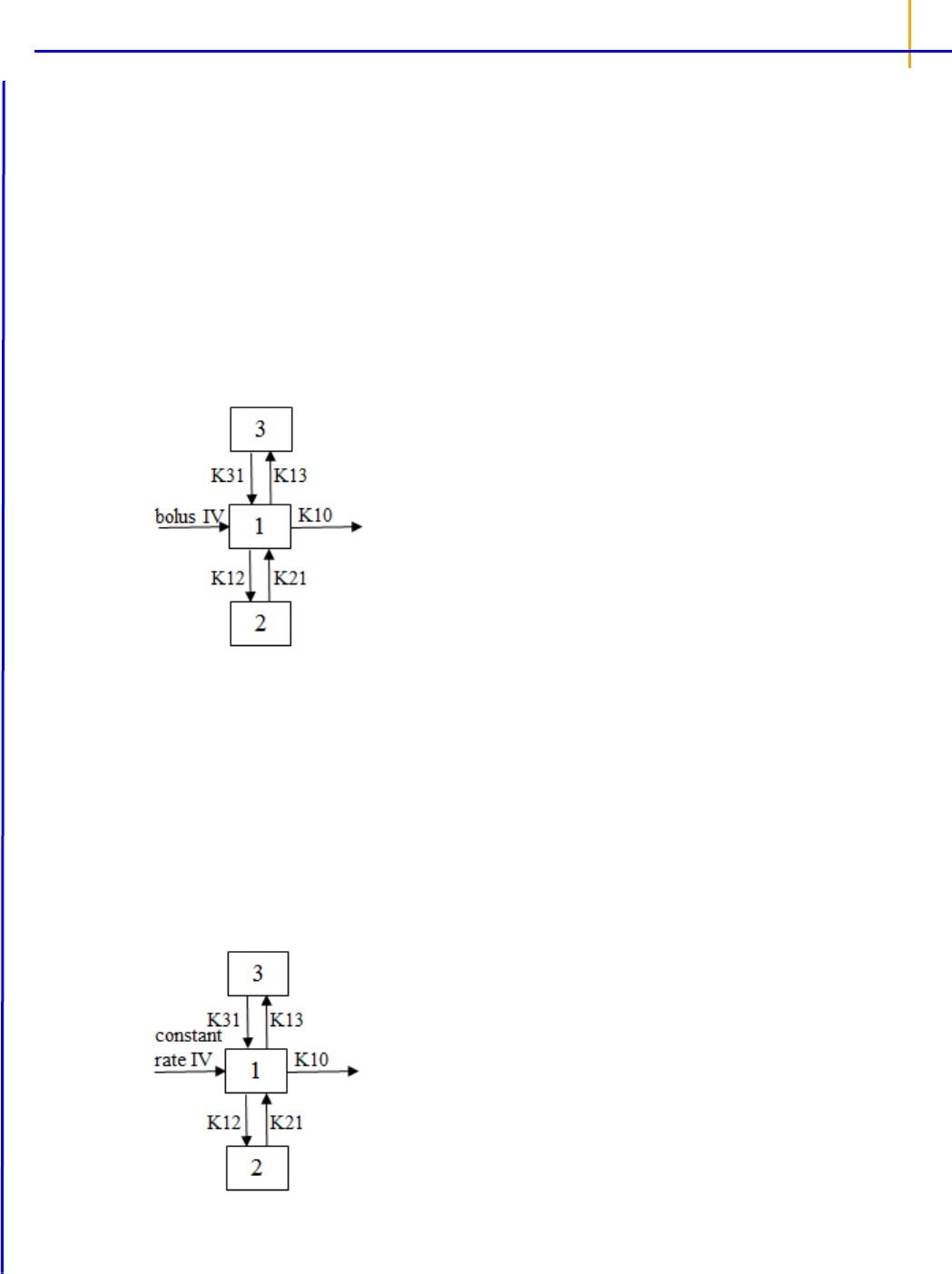
239

Model 17

Two-compartment with simultaneous bolus IV and constant infusion input and macro constants as pri-

mary parameters.

Model 10 with macroconstants as the primary (estimated) parameters.

Required constants: Stripping dose, bolus dose, IV dose, length of infusion (= Tinf)

Estimated parameters: A, B, Alpha, Beta

Secondary parameters: K10, K12, K21, K10 half-life, Alpha half-life, Beta half-life, V1, CL, V2, CLD2

Clearance parameters are not available in Model 17.

Model 18

Three-compartment with bolus input, first-order output; macro constants as primary parameters.

Required constants: Stripping dose,

N doses, dose N, time of dose N (Repeat for each dose)

Estimated parameters: A, B, C, Alpha, Beta, Gamma

Secondary parameters: Cmax, V1, K21, K31, K10, K12, K13, K10 half-life, Alpha half-life, Beta half-

life, Gamma half-life, AUC, CL, AUMC, MRT, Vss, V2, CLD2, V3, CLD3

Clearance parameters are not available in Model 18.

Model 19

Three compartment model with constant IV infusion; macro constants as primary parameters.

Ct A t–exp B t–exp+ C t–exp+=

Phoenix WinNonlin

User’s Guide

240

where:

Tinf = infusion length

t* = t – Tinf for t > Tinf 

t* = 0 for t  Tinf

Required constants:

N doses, dose N, start time and end time of dose N (Repeat for each dose)

Estimated parameters: V1, K21, K31, Alpha, Beta, Gamma

Secondary parameters: Cmax, K10, K12, K13, A, B, C, K10 half-life, Alpha half-life, Beta half-life,

Gamma half-life, AUC, CL, AUMC, MRT, Vss, V2, CLD2, V3, CLD3

A, B, and C are the zero time intercepts following an IV injection.

Clearance parameters are not available in Model 19.

Ct A

t*–exp t–exp–

t*–exp t–exp–

t*– t–exp–exp

Tinf

----------

K21 –K31 –

V  ––

--------------------------------------------------





Tinf

----------

K21 –K31 –

V  ––

-------------------------------------------------





Tinf

----------

K21 –K31 –

V  ––

-----------------------------------------------





241

PD output parameters in a PK/PD model

The output parameters for PD models in a linked PK/PD model differ from the parameters for PD

models that are not linked. The following list shows the PD model parameters used in linked PK/PD

models.

101 Simple Emax model

Estimated parameters: Emax, EC

, Ke0

102 Simple Emax model with a baseline effect

Estimated parameters: Emax, EC

50,

E0, Ke0

Secondary parameters: Rmax, F_Emax

103 Inhibitory effect E0 model

Estimated parameters: E0, IC

, Ke0

104 Inhibitory effect Imax model with a baseline effect

Estimated parameters: Imax, IC

, E0, Ke0

Secondary parameters: Rmax, F_Emax

105 Sigmoid Emax model

Estimated parameters: Emax, EC

, Gamma, Ke0

106 Sigmoid Emax model with a baseline effect

Estimated parameters: Emax, EC

e50

, E0, Gamma, Ke0

Secondary parameters: Rmax, F_Emax

107 Inhibitory effect sigmoid E0 model

Estimated parameters: E0, IC

, Gamma, Ke0

108 Inhibitory effect sigmoid Imax model with a baseline effect

Estimated parameters: Imax, IC

, E0, Gamma, Ke0

Secondary parameters: Rmax, F_Emax

Below are definitions for the estimated and secondary parameters.

Emax: Maximum drug effect.

Imax: Maximum drug inhibition.

: Concentration in plasma that achieves 50% of predicted maximum effect in an Emax model.

ECe

: For effect compartment models, the concentration at the effect site that achieves 50% of pre-

dicted maximum effect in an Emax model.

: Drug concentration required to produce 50% of the maximal inhibition.

: Baseline effect (effect at 0). In models 103 and 107, E0 could also be named Imax, the maximum

drug inhibition.

Gamma: Shape parameter.

Ke0: Exit rate constant from effect compartment.

Rmax: Observed or predicted maximum response.

F_Emax: Fractional change in response from baseline E

Phoenix WinNonlin

User’s Guide

242

ASCII Model dosing constants

The number of constants in the model corresponds to the dosing route for the model.

Bolus and first-order input models require at least three dosing constants per profile.

CON[0]: Number of doses (N)

CON[1]: Dose amount for dose N

CON[2]: Time of dose for dose N

CON[3]: Dose amount for dose N+1 (if multiple doses are used)

CON[4]: Time of dose for dose N+1 (if multiple doses are used)

Constant IV infusion models require at least four dosing constants per profile.

CON[0]: Number of doses (N)

CON[1]: Dose amount for dose N

CON[2]: Start time for dose N

CON[3]: End time for dose N

CON[4]: Dose amount for dose N+1 (if multiple doses are used)

CON[5]: Start time for dose N+1 (if multiple doses are used)

CON[6]: End time for dose N+1 (if multiple doses are used)

243

Parameter Estimates and Boundaries Rules

Rules for using parameter estimates and boundaries in Indirect Response, Linear, Michaelis-Menten,

PD, PK, PK/PD, and ASCII models include the following:

• Using boundaries, either user- or WinNonlin-generated, is recommended.

• Phoenix uses curve stripping only for single-dose data. If multiple dose data is fit to a PK model

and Phoenix generates initial parameter estimates, a grid search is performed to obtain initial esti-

mates. In this case, boundaries are required.

• For linear regressions, it is recommended that users keep the Do Not Use Bounds option

checked in the Parameter Options tab and select minimization method 3 (Gauss-Newton (Hart-

ley)) in the Engine Settings tab.

• The grid used in grid searching uses three values for each parameter. If four parameters are esti-

mated, the grid contains 3

=81 possible points. The point on the grid associated with the smallest

sum of squares is used as an initial estimate for the estimation algorithm. This option is included

for convenience, but it might greatly slow the parameter estimation process if the model is defined

in terms of differential equations.

• If the data are fitted to a micro-constant model, Phoenix performs curve stripping for the corre-

sponding macro-constant model then uses the macro-constants to compute the micro-constants.

It is recommended that users specify the Lower and Upper boundaries, even when Phoenix

computes the initial estimates.

• If the Gauss-Newton methods (minimization methods 2 and 3) are used to estimate the parame-

ters, then the boundaries are determined by applying a normit transform to the parameter space.

• If the Nelder-Mead method (minimization method 1) is selected, the residual sum of squares is

set to a large number if any of the parameter estimates go outside the specified constraints at any

iteration, which forces the parameters back within the specified bounds.

• Unlike the linearization methods, the use of bounds does not affect numerical stability when using

the Nelder-Mead method. Using bounds with the Nelder-Mead method will keep the parameters

within the bounds. The use of bounds, either user-supplied or Phoenix-supplied, is always recom-

mended with the Gauss-Newton methods.

References

Beck and Arnold (1977). Parameter Estimation in Engineering and Science. John Wiley & Sons, New

York.

Bard (1974). Nonlinear Parameter Estimation. Academic Press, New York.

Bates and Watts (1988). Nonlinear Regression Analyses and Its Applications. John Wiley & Sons,

New York.

Davies and Whitting (1972). A modified form of Levenberg's correction. Chapter 12 in Numerical

Methods for Non-linear Optimization. Academic Press, New York.

Dayneka, Garg and Jusko (1993). Comparison of four basic models of indirect pharmacodynamic

responses. J Pharmacokinet Biopharm 21:457.

Draper and Smith (1981). Applied Regression Analysis, 2nd ed. John Wiley & Sons, NY.

Endrenyi, ed. (1981). Kinetic Data Analysis: Design and Analysis of Enzyme and Pharmacokinetic

Experiments. Plenum Press, New York.

Gabrielsson and Weiner (2016). Pharmacokinetic and Pharmacodynamic Data Analysis: Concepts

and Applications, 5

ed. Apotekarsocieteten, Stockholm.

Phoenix WinNonlin

User’s Guide

244

Gill, Murray and Wright (1981). Practical Optimization. Academic Press.

Hartley (1961). The modified Gauss-Newton method for the fitting of nonlinear regression functions

by least squares. Technometrics 3:269–80.

Jennrich and Moore (1975). Maximum likelihood estimation by means of nonlinear least squares.

Amer Stat Assoc Proceedings Statistical Computing Section 57–65.

Jusko (1990). Corticosteroid pharmacodynamics: models for a broad array of receptor-mediated

pharmacologic effects. J Clin Pharmacol 30:303.

Kennedy and Gentle (1980). Statistical Computing. Marcel Dekker, New York.

Metzler and Tong (1981). Computational problems of compartmental models with Michaelis-Menten-

type elimination. J Pharmaceutical Sciences 70:733–7.

Nelder and Mead (1965). A simplex method for function minimization. Computing Journal 7:308–13.

Ratkowsky (1983). Nonlinear Regression Modeling. Marcel Dekker, New York.

Shampine, Watts and Davenport (1976). Solving nonstiff ordinary differential equations - the state of

the art. SIAM Review 18:376–411.

Tong and Metzler (1980). Mathematical properties of compartment models with Michaelis-Menten-

type elimination. Mathematical Biosciences 48:293–306.

PK model examples

245

PK model examples

Knowledge of how to do basic tasks using the Phoenix interface, such as creating a project and

importing data, is assumed.

Fit a PK model to data example

Simulation and study design of PK models example

More nonlinear model examples

Fit a PK model to data example

This example is about creating and saving PK models in Phoenix and supposes that a researcher has

obtained concentration data from one subject after oral administration of a compound, and now

wishes to fit a pharmacokinetic (PK) model to the data.

The completed project (

PK_Model.phxproj) is available for reference in …\Examples\Win-

Nonlin

Explore the PK input data

Create a new project called PK Model.

2. Import the file …\Examples\WinNonlin\Supporting files\study1.CSV.

In the File Import Wizard dialog, select the Has units row option and click Finish.

3. Right-click study1 in the Data folder and select Send To > Plotting > XY Plot.

4. In the XY Data Mappings panel:

Leave Subject mapped to the None context.

Map Time to the X context.

Map Conc to the Y context.

5. Click (Execute icon) to execute the object.

6. In the Options tab below the plot, select Axes > Y from the menu tree.

7. Select the Logarithmic option button in the Scale area. Leave the logarithmic base set to 10.

The XY Plot is automatically updated to reflect the scale change.

Set up the object

The plots suggests that the system might be adequately modeled by a one-compartment, 1st order

absorption model. This model is available as Model 3 in the pharmacokinetic models included in

Phoenix. Set up a PK Model object and a Maximum Likelihood Model object, for comparison.

PK Model object

1. Right-click study1 in the Data folder and select Send To > Modeling > Least Squares Regres-

sion Models > PK Model.

2. In the Main Mappings panel:

Map Subject to the Sort context.

Leave Time mapped to the Time context.

Map Conc to the Concentration context.

3. In the Model Selection tab below the Setup panel, check the Number 3 model checkbox.

Entering the units for dosing data makes it possible to view and adjust units for the model parameters.

In this example, a single dose of 2 micrograms was administered at time zero.

Phoenix WinNonlin

User’s Guide

246

1. Select the Dosing panel in the Setup tab.

2. Check the Use Internal Worksheet checkbox.

3. Click OK in the Select sorts dialog to accept the default sort variable.

4. In the cell under Time type 0.

5. In the cell under Dose type 2.

6. In the Weighting/Dosing Options tab below the Setup panel, type ug in the Unit field.

All model estimation procedures benefit from initial estimates of the parameters. While Phoenix can

compute initial parameter estimates using curve stripping, this example will provide user values for

the initial parameter estimates.

1. Select the Parameter Options tab below the Setup panel.

2. Select the User Supplied Initial Parameter Values option.

The WinNonlin Bounds option is selected by default as the Parameter Boundaries. Do not

change this setting.

3. Select Initial Estimates in the Setup panel list.

4. Check the Use Internal Worksheet checkbox.

5. Click OK to accept the default sort variable in the Select sorts dialog.

6. Enter the following information in the table:

For row 1 (V_F), enter

0.25 in the Initial column.

For row 2 (K01), enter

1.81 in the Initial column.

For row 3 (K10), enter

0.23 in the Initial column.

Maximum Likelihood Models object

1. Right-click the study1 worksheet in the Data folder and select Send To > Modeling > Maximum

Likelihood Models.

2. In the Structure tab, uncheck the Population box.

3. Click the Set WNL Model button.

The contents of the Structure tab changes. The first of the two untitled menus allows users to

select a PK model, and the second allows users to select a PD model.

4. In the first untitled menu, select 3 (1cp extravascular).

5. Click Apply to set the WinNonlin model.

6. Use the option buttons in the Main Mappings panel to map the data types to the following contexts:

Subject to the Sort context.

Time to the Time context.

Conc to the CObs context.

PK model examples

247

The WARNINGS tab at the bottom highlights potential issues. If there are no issues, the tab will be

labeled “no warnings”. Click the WARNINGS tab and note the message that Aa values are missing.

This will be taken care of in the next few steps.

In this example, a single dose of 2 micrograms was administered at time zero. However, since the

concentration units were ng/mL, the dose should be entered as 2000ng so the units are equivalent.

1. Select the Dosing panel in the Setup tab.

2. Check the Use Internal Worksheet checkbox.

3. In the cell under Aa type 2000.

4. In the cell under Time type 0.

5. Click View Source above the worksheet.

6. In the Columns tab below the table, select Aa from the Columns list and enter ng in the Unit field.

7. Click X in the upper right corner to close the source window (the units are added to the column

header).

Notice that the warning about Aa values is gone and the tab label now says “no warnings.”

The Maximum Likelihood Models engine will not generate its own initial estimates, like the Least-

Squares Regression Model engine can, so it is important to consider reasonable starting values.

1. Select the Initial Estimates tab in the lower panel.

2. Extend the Duration to 15, since the last observed timepoint is 14 hours.

3. Enter values 2, 300, and 0.1 for tvKa, tvV, and tvKe, respectively.

Note: Make sure the tvKe box is checked after entering the value. Entering a leading “0” for a value

causes the corresponding checkbox to automatically be cleared.

The y axis can also be set to log scale and, if there is more than one profile, the curves can be

overlaid by checking the log and overlay boxes, respectively.

Phoenix WinNonlin

User’s Guide

248

Note how the predicted curve roughly follows the observed data now.

4. Click the blue arrows to submit these values to the main model engine (if the arrow is blue, then

the value will not be used).

Execute and view the results

At this point, all of the necessary commands and options have been specified.

1. Execute each object in the workflow.

The Results tab contains three types of model output:

Worksheets (descriptions of the worksheets are located in the

“Worksheet output” section) 

Plots

Text output

The six plots generated by the PK Model object are shown below. The NLME object generates more

plots, however the ones corresponding to the WinNonlin output are listed in parentheses.

Figure 39-1. Observed Y and Predicted Y vs X (Ind DV, IPRED vs TAD)

PK model examples

249

Figure 39-2. Partial Derivatives plot (Ind Partial Derivatives)

Figure 39-3. Predicted Y vs Observed Y (Ind DV vs IPRED, axes swapped)

Phoenix WinNonlin

User’s Guide

250

Figure 39-4. Predicted Y vs X

Figure 39-5. Residual Y vs Predicted Y (Ind IWRES vs IPRED)

PK model examples

251

Figure 39-6. Residual Y vs X (Ind IWRES vs TAD)

The tables generated by the ML Model object summarize useful information.

Overall: Contains -2LL (the objective function) and other goodness of fit information 

Theta: Final parameter estimates

Residuals: Analogous to Summary Table of Least-Squares Regression and NCA models

To compare the two models, create a worksheet by appending the Final Parameters worksheet from

the PK model to the Theta worksheet from the ML Model object. (See

“Append Worksheets” for spe-

cifics on how to append worksheets.)

The Core Output text file contains all model settings and output in plain text format. Below is part of

the Core Output file from the ML Model object run.

Phoenix WinNonlin

User’s Guide

252

Save the project and the results

Projects and their results can be saved as a project file or loaded into Integral.

To save the project as a file, select File > Save Project.

For details on adding the project to Certara Integral, see

“Adding a project to Integral”.

Simulation and study design of PK models example

Considerable research has been done in the area of optimal designs for linear models. Most methods

involve computation of the variance covariance matrix. The “optimal” design is usually one in which

replicate samples are taken at a limited number of combinations of experimental conditions. Unfortu-

nately, these methods are of little or no value when designing experiments involving nonlinear models

for a number of reasons, including:

• It can be difficult or, in the case of a pharmacokinetic study, impossible to obtain replicate

observations.

• The primary interest often is not in the model parameters but in some functions of the model

parameters such as AUC, t

1/2

, etc.

When Phoenix performs a simulation, the output includes information on precisely how parameters in

the model can be estimated for specified values of the independent variables, such as time.

Assume that a study is being planned and that the data produced by this study should be consistent

with Phoenix PK model 3. Assume also that the parameter values should be approximately: V_F=10,

K01=3, K10=0.05 and one of the following study designs, or sampling times, will be used:

0, 1.5, 3, 6, 9, 12, 15, 18, and 24 hours 

or

0, 0.5, 1, 2, 4, 8, 12, 24, and 36 hours.

PK model examples

253

Simulation can be used to determine which set of sampling times would produce the more precise

estimates of the model parameters. This example will use Phoenix to simulate the model with each

set of sampling times, and compare the variance inflation factors for the two simulations.

The completed project (

Study_Design.phxproj) is available for reference in …\Exam-

ples\WinNonlin

Create the input dataset

Follow the following steps to create the dataset. Alternatively, the data can be imported from

…\Examples\WinNonlin\Supporting files\Example Data.csv.

1. Create a new project with the name Study Design.

2. Right-click the Data folder in the Object Browser and select New > Worksheet.

3. Name the new worksheet Example Data.

4. In the Columns tab, add a column identifying the group number by clicking Add underneath the

Columns list.

5. In the New Column Properties dialog, type Group in the Column Name field. Leave the data type

set to Numeric, and click OK.

6. In the first cell under Group, type 1 and press ENTER. Continue to enter 1 for rows 2–9.

7. In rows 10–18 type 2 in the Group column.

8. Add a column of time data by clicking Add underneath the Columns list.

9. In the Column Name field, type Times. Leave the data type set to Numeric and click OK.

10. Type the values 0, 1.5, 3, 6, 9, 12, 15, 18, and 24 in the Times column for rows 1–9 and values 0,

0.5, 1, 2, 4, 8, 12, 24, and 36 for rows 10–18.

Set up the object

This model is available as Model 3 in the pharmacokinetic models included in Phoenix.

1. Right-click Example Data in the Data folder and select Send To > Modeling > Least Squares

Regression Models > PK Model.

2. In the Main Mappings panel:

Map Group to the Sort context.

Map Times to the Time context.

3. In the Model Selection tab below the Setup panel, specify the PK model that Phoenix will use in

the analysis by selecting the Number 3 model checkbox.

4. Select the Simulation checkbox on the right side of the Model Selection tab (notice that the Con-

centration mapping is changed from required (orange) to option (gray)).

5. In the Y Units field, type ng/mL.

6. Enter the dosing data by selecting the PK Model's Dosing panel in the Setup tab.

7. Check the Use Internal Worksheet checkbox.

8. Click OK in the Select sorts dialog to accept the default sort variable.

9. In the Time column type 0 for both groups.

10. In the Dose column type 100 for both groups.

Phoenix WinNonlin

User’s Guide

254

Note: The number of rows in the Group column corresponds to the number of doses received. For

example, if group 1 had 10 doses, there would be 10 rows of dosing information for group 1. In

Phoenix this grouping of data is referred to as stacking data.

11. In the Weighting/Dosing Options tab below the Setup panel, type mg in the Unit field.

12. Select the Parameter Options tab.



Parameter values must be specified for simulations. The User Supplied Initial Parameter Values

option is selected and cannot be changed. The Do Not Use Bounds option is selected by default

and cannot be changed.



Selecting the Simulation checkbox makes the parameter calculation and boundary selection

options unavailable. If the Simulation checkbox is selected, then users must supply initial param-

eter values, and parameter boundaries are not used.

13. Select Initial Estimates in the Setup list.

14. Check the Use Internal Worksheet checkbox.

15. In the Select sorts dialog, click OK to accept the default sort variable.

16. Enter the following initial values for each group: V_F=10, K01=3, K10=0.05.

Execute and view the results

All the settings are complete and the model can be executed.

1. Execute the object.

The variance inflation factors (VIF) for each dosing scheme (groups 1 and 2) are located in the Final

Parameters worksheet and are summarized (with values rounded) below.

V_F 

Estimate = 10

Group 1 VIF = 0.779

Group 2 VIF = 0.657

K01 

Estimate = 3

Group 1 VIF = 68.48

Group 2 VIF = 1.176

K10 

Estimate = 0.05

Group 1 VIF = 0

Group 2 VIF = 0

In practice, it is useful to vary the values of V_F, K01, and K10 and repeat the simulations to deter-

mine if the first set of sampling times consistently yields less precise estimates than the second set.

Design the sampling plan

Note that, for the parameters V_F and K10, the estimated variances would be approximately 15%

lower using the second set of times, while the difference is much more dramatic for the parameter

K01. These sets of variance inflation factors indicate that the second set of sampling times would pro-

vide tighter estimates of the model parameters.

PK model examples

255

The partial derivatives plots for this model explain this result. The locations at which the partial deriva-

tive plots reach a maximum or a minimum indicate times the model is most sensitive to changes in the

model parameters, so one approach to designing experiments is to sample where the model is most

sensitive to changes in the model parameters.

1. Click Partial Derivatives Plot in the Results tab.

Figure 39-7. Partial Derivatives plot Group 1

2. Select the Page 02 tab below the plot.

Note that in the first plot of the partial derivatives the model is most sensitive to changes in K10 at

about 20 hours. Both sampling schemes included times near 20 hours, so therefore the two sets

of sampling times were nearly equivalent in the precision with which K10 would be estimated.

Phoenix WinNonlin

User’s Guide

256

For both V_F and K01 the model is most sensitive to changes very early, at about 0.35 hours for

K01 and about 1.4 hours for V_F. The first set of sampling times does not include any post-zero

points until hour 3, long past these areas of sensitivity. Even the second set of times could be

improved if samples could be taken earlier than 0.5 hours.

This same technique could be used for other models in Phoenix or for user-defined models.

3. Close this project by right-clicking the project and selecting Close Project.

More nonlinear model examples

Knowledge of how to do basic tasks using the Phoenix interface, such as creating a project and

importing data, is assumed.

The examples project

Model_Examples.phxproj located in …\Examples\WinNonlin

involve Least-Squares Regression modeling objects. Each model object within this project contains

the appropriate default mappings and settings needed to run the model.

To run these example objects:

1. Load the project …\Examples\WinNonlin\Model_Examples.phxproj into Phoenix.



Each example model has the following items associated with it:

• A dataset in workbook form.

• Many have datasets in workbook form for dosing.

• A PK, PKPD, Indirect Response, or User ASCII model object.

2. Explore each model object and its mappings and settings.

3. Execute each model.

Explanations for each model object in the example is given below.

Pharmacokinetic model (Exp1)

In the Exp1 example, a dataset was fit to PK model 13 in the pharmacokinetic model library. Four con-

stants are required for model 13: the stripping dose associated with the parameter estimates, the

number of doses, the dose, and the time of dosing.

This example uses weighted least squares (1/observed Y). Phoenix determines initial estimates via

curve stripping and then generates bounds for the parameters.

Pharmacokinetic model with multiple doses (Exp2)

In the Exp2 example, a dataset obtained following multiple dosing is fit to model 13 in the pharmaco-

kinetic model library, which is a two-compartment open model. This model has five parameters: A, B,

K01, Alpha, and Beta and uses the user-supplied initial values

20, 5, 3, 2, and 0.05. Phoenix gen-

erates bounds for the parameters.

Probit analysis: maximum likelihood estimation of potency (Exp3)

The Exp3 example demonstrates how to use the NORMIT and WTNORM functions to perform a pro-

bit regression (parallel line bioassay or quantal bioassay) analysis. Note that a probit is a normit plus

five. There are several interesting features used in this example:

• The transform capability was used to create the response variable.

• The logarithm of the relative potency is estimated as a secondary parameter.

PK model examples

257

• Maximum likelihood estimates were obtained by iteratively reweighting and turning off the halv-

ings and convergence criteria. Therefore, instead of iterating until the residual sum of squares is

minimized, the program adjusts the parameters until the partial derivatives with respect to the

parameters in the model are zero. This will normally occur after a few iterations.

• Since there is no



in a problem such as this, variances for the maximum likelihood estimates

are obtained by setting S

=1 (MEANSQUARE=1).

• The following modeling options are used:

• Method 3 is selected, which is recommended for Maximum Likelihood estimation (MLE), and

iterative reweighting problems.

• Convergence Criterion is set to 0. This turns off convergence checks for MLE.

• Iterations are set to 10. Estimates should converge after a few iterations.

• Meansquare is set to 1. Sigma squared is 1 for MLE.

For further reading regarding use of nonlinear least squares to obtain maximum likelihood estimates,

refer to Jennrich and Moore (1975). Maximum likelihood estimation by means of nonlinear least

squares. Amer Stat Assoc Proceedings Statistical Computing Section 57–65.

Logit regression (bioassay) (Exp4)

1 p–

------------log X+=

The following data were obtained in a toxicological experiment:

In the Exp4 example, assume that the distribution of Y is binomial with:

mean =



variance = npq, and q=1 – p

where:

and

X = log

dose

Maximum likelihood estimates of

 and  for this model are obtained via iteratively reweighted least

squares. This is done by fitting the mean function (

np) to the Y data with weight (npq)

–1

The modeling commands needed to fit this model to the data are included in an ASCII model file. Note

that the log

LD50 and log

LD001 are also estimated as secondary parameters.

This model is really a linear logit model in that:

X+exp

1 X+exp+

-----------------------------------------

Phoenix WinNonlin

User’s Guide

258

Note: For this type of problem, the final value of the residual sum of squares is the Chi-square statistic

for testing heterogeneity of the model. If this example is run a user obtains X

(heterogene-

ity)=2.02957, with 4 – 2=2 degrees of freedom (number of data points minus the number of param-

eters that were estimated).

For a more in-depth discussion of the use of nonlinear least squares for maximum likelihood estima-

tion, see Jennrich and Moore (1975). Maximum likelihood estimation by means of nonlinear least

squares. Amer Stat Assoc Proceedings Statistical Computing Section 57–65.

In the Engine Settings tab, the Convergence Criteria is set to zero to turn off the halving and conver-

gence checks. Meansquare is set to 1 (the residual mean square is redefined to be 1.00) in order to

estimate the standard errors of

a, b, and the secondary parameters.

Survival analysis (Exp5)

Exp5 is another maximum likelihood example and is very similar t

o Model Exp4. It is included to show

that models arising in a variety of disciplines, such as case survival or reliability analysis, can be fit by

nonlinear least squares.

The dosing constant is defined in this model as the denominator for the proportions, that is,

In the Engine Settings tab the Convergence Criteria is set to zero to turn off the halving and conver-

gence checks. Meansquare is set to 1 (redefines the residual mean square to be 1.00) in order to esti-

mate the standard errors of the primary and secondary parameters.

Two differential equations with data for both compartments (Exp6)

---------

K12– Z

=

Exp6 involves the following model:

where K12 and K20 are first-order rate constants. This model may be described by the following

system of two differential equations.

compartment 1

---------

K12 Z

 K20 Z

–=

compartment 2

with initial conditions

=D, and Z

=0.

In addition to obtaining estimates of K12 and K20, it is also desirable to estimate

D and the half-lives

of K12 and K20.

A sample solution for this example is given here. Note that, for this example, the model is defined as

an ASCII file. Data corresponding to both compartments are available.

Column C in the dataset for this example contains a function variable, which defines the separate

functions.

Two differential equations with data on one-compartment (Ex7)

The model for the Exp7 example is identical to that for Exp6. However, in this example, it is assumed

that data are available only for compartment two.

PK model examples

259

Multiple linear regression (Exp8)

i 1=



Linear regression models are a subset of nonlinear regression models; consequently, linear models

can also be fit using Phoenix. To illustrate this, a sample dataset (taken from Analyzing Experimental

Data By Regression by Allen and Cady (1982), Lifetime Learning Publications, Belmont, CA) was

analyzed in Exp8. Note that linear models can always be written as:

This example is also interesting in that the model was initially defined in such a way to permit several

different models to be fit to the data.

In the ASCII model panel, note that the number of parameters to be estimated is defined in CONS in

order to make the model specification as general as possible. Note also the use of a DO loop in the

model text.

Note: When using Phoenix to fit a linear regression model:

- use arbitrary initial values 

- make sure the Do Not Use Bounds option is checked

- select the Gauss-Newton minimization method with the Levenberg and Hartley modification

The dosing constant for this example is the number of terms to be fit in the regression.

Cumulative areas under the curve (Exp9)

The Exp9 example uses the TRANSFORM

block of commands to output cumulative area under the

curve values calculated by trapezoidal rule. It computes cumulative urine excretion then fits it to a

one-compartment model. The use of the LAG function is demonstrated.

Mitscherlich nonlinear model (Exp10)

– – xexp=

In the Exp10 example, a dataset is fit to the Mitscherlich model. The data were taken from Allen and

Cady (1982), Analyzing Experimental Data By Regression. Lifetime Learning Publications, Belmont,

CA. Fitting data to this model involves the estimation of three parameters;

, b

, and .

Four parameter logistic model (Exp11)

ad–

1 xc

--------------------------

d+=

The Exp11 example illustrates how to fit a dataset to a general four parameter logistic function. The

function is often used to fit radioimmunoassay data. The function, when graphed, depicts a sigmoidal

(S-shaped) curve. The four parameters represent the lower and upper asymptotes, the ED50, and a

measure of the steepness of the slope. For further details see DeLean, Munson and Rodbard (1978).

Simultaneous analysis of families of sigmoidal curves: Application to bioassay, radioligand assay and

physiological dose-response curves. Am J Physiol 235(2):E97–E102. The model, with parameters

b, c, and d is as follows:

Phoenix WinNonlin

User’s Guide

260

Linear regression (Exp12)

The Exp12 example is based on work published by Draper and Smith (1981). Applied Regression

Analysis, 2nd ed. John Wiley & Sons, NY.

Note: When doing linear regression in Phoenix, enter arbitrary initial estimates and make sure the Do

Not Use Bounds option is checked. Use the Gauss-Newton minimization method with the Leven-

berg and Hartley modification

Indirect response model (IR)

The IR example is PD8 from the textbook: Gabrielsson and Weiner (2016). Pharmacokinetic and

Pharmacodynamic Data Analysis: Concepts and Applications, 5

ed. Apotekarsocieteten, Stockholm.

It uses an indirect response model, linking Phoenix pharmacokinetic model 11 to indirect response

model 54. The PK data were fit in a separate run and are linked to the Indirect Response model. This

can be done via the PKVAL command when using an ASCII model or via the PK parameters panel.

Model 11 is a two-compartment micro constant model with extravascular input.

Ke0 link model (PKPD)

The PKPD example is PD10 from the textbook: Gabrielsson and Weiner (2016). Pharmacokinetic and

Pharmacodynamic Data Analysis: Concepts and Applications, 5

ed. Apotekarsocieteten, Stockholm.

It uses an effect compartment PK/PD link model. The drug was administered intravenously, and a

one-compartment model is assumed (PK Model 1). The PD data is fit to a simple Emax model (PD

Model 101). The pharmacokinetic data were fit in a separate run and are linked to the pharmacody-

namic model.

Pharmacokinetic/pharmacodynamic link model (Exp15)

Rather than fitting the PK data to a PK model, an effect compartment is fitted and Ke0 estimated in

the Exp15 example using the observed Cp data. Therefore it is a type of nonparametric model. The

collapsed Ce values are then used to model the PD data. The example also illustrates how to mix dif-

ferential equations and integrated functions. This approach was proposed by Dr. Wayne Colburn.

261

Core Output File

The Core Output is an ASCII text file that contains a complete summary of the model commands,

options, parameters, and values for a model, as well as any errors that occurred during modeling.

This file is generated as output for Indirect Response, Linear, Michaelis-Menten, PD, PK, PKPD, and

ASCII Model objects.

Sections of the Core Output file include:

List of input commands

Minimization process

Final parameters

Variance-covariance matrix, correlation matrix, and eigenvalues

Residuals

Secondary parameters

List of input commands

The first section lists the input commands used to run the model. See “Commands, Arrays, and Func-

tions”

for an alphabetic listing of commands.

Minimization process

This section varies depending on the selected minimization method. If a Gauss-Newton method is

used (methods 2 or 3), this page shows the parameter values and the computed weighted sum of

squared residuals at each iteration. In addition, the following two values are listed for each iteration:

RANK: The rank of the matrix of partial derivatives of the model parameters. If the matrix is of full

rank, then the rank equals the number of parameters. If the rank is less than the number of

parameters, then the problem is ill-conditioned. That means there is not enough information con-

tained in the data to precisely estimate all of the parameters in the model.

CONDITION NO.: Condition number of the matrix of partial derivatives. The condition number is

the square root of the ratio of the largest to the smallest eigenvalue of the matrix of partial deriva-

tives. If the condition number gets to be very large, for example greater than 10E+06, then the

estimation problem is very ill-conditioned. If minimization methods 2 or 3 are used, then using

lower and upper parameter boundaries can help reduce the condition number.

If the Nelder-Mead method is used, this section only shows the parameter values and the weighted

sum of squares for the initial point, final point (the best or smallest sum of squares), and the next-to-

best point.

Final parameters

This section lists the parameter estimates, the asymptotic estimated standard error of each estimate,

and two intervals based on this estimated standard error. The intervals labeled UNIVAR_CI_LOW and

UNIVAR_CI_UPP are the parameter estimates plus and minus the product of the estimated standard

error and the appropriate value of the t-statistic. Univariate intervals should be applied individually to

the relevant single parameters, and have the interpretation that there is a 95% probability that the

interval contains the true value of the individual parameter.

The intervals labeled PLANAR_CI_LOW and PLANAR_CI_UPP are obtained from the tangent planes

to the joint 95% ellipsoid of all the parameter estimates. The intervals are defined by the parameter

estimates plus and minus the product of the standard error and the appropriate value of an F-statistic.

The PLANAR intervals in general are larger than the corresponding UNIVARIATE intervals and jointly

Phoenix WinNonlin

User’s Guide

262

define a region in the shape of a rectangular box that contains the joint ellipsoid. This PLANAR region

has the interpretation there is at least a 95% probability that this box contains the true parameter vec-

tor formed from the individual parameter values.

For an introductory discussion of the issues involved in UNIVARIATE and PLANAR intervals see page

95 (Draper and Smith (1981)). Details of the appropriate F-distribution statistic used in the PLANAR

ellipsoidal and box region computations can be found in most advanced statistical texts.

The estimated standard errors and intervals are only approximate, because they are based on a lin-

earization of a nonlinear model. The closer the model is to being linear, the better the approximation.

See Chapter 10 of Draper and Smith (1981) for a complete discussion of the true intervals for param-

eter estimates in nonlinear models.

The estimated standard errors are valuable for indicating how much information about the parameters

is contained in the data. Many times a model provides a good fit to the data in the sense that all of the

deviations between observed and predicted values are small, but one or more parameter estimates

have standard errors that are large relative to the estimate.

Variance-covariance matrix, correlation matrix, and eigenvalues

The next three sections of the Core Output show the correlation matrix of the estimates and the

eigenvalues of the linearized form of the model. High correlations among one or more pairs of the

estimates indicate that the UNIVAR limits are underestimates of the uncertainty in the parameter esti-

mates and, although the data may be well fit by the model, the estimates may not be very reliable.

Also, datasets that result in highly correlated estimates are often difficult to fit, in the sense that the

Gauss-Newton algorithm will have trouble finding the minimum residual sum of squares.

The eigenvalues are another indication of how well the data define the parameters. If the parameter

estimates are completely uncorrelated, then the eigenvalues are equal. A large ratio between the

largest and smallest eigenvalue may indicate that there are too many parameters in the model. How-

ever, it is usually not possible to remove one parameter from a nonlinear model. For discussion of the

use of eigenvalues in modeling see (Belsley, Kuh and Welsch (1980)).

Residuals

This section of the output lists the observed data, calculated predicted values of the model function,

residuals, weights, the standard deviations (S) of the calculated function values and standardized

residuals. Runs of positive or negative deviations indicate non-random deviations from the model and

are indicators of an incorrect model and/or choice of weights.

Also in this section are the sum of squared residuals, the sum of weighted squared residuals, an esti-

mate of the error standard deviation, and the correlation between observed and calculated function

values. In nonlinear models the correlation is not a particularly good measure of fit. In most problems

it is greater than 0.9, and anything less than 0.8 probably indicates serious problems with the data

and/or model. Two statistical criterion for model selection and comparison, the AIC (Akaike (1978))

and SBC (Schwarz (1978)), are also listed in this section.

If the data is fit to a model for extravascular or constant infusion input, area under the curve (AUC) is

listed at the end of this section of the Core Output. The AUC is computed by the linear trapezoidal

rule. If the first time value is not zero, then WinNonlin generates a data point with time and concentra-

tion values of zero, to compute AUC from zero to the last time. Note that this AUC in the Core Output

differs from the AUC in the Secondary Parameters results worksheet. The secondary parameter AUC

is calculated using the model parameters.

Note: AUC values are always associated with the first dose and might not be meaningful if the data were

obtained after multiple dosing or IV dosing, due to time zero extrapolation problems.

263

Secondary parameters

Any secondary parameters and their estimated asymptotic standard errors are listed in the last sec-

tion. The secondary parameters are functions of the primary parameters listed in the Core Output. In

the case of multiple-dose data, secondary parameters that depend on dose use the first dose in their

computation. The standard errors of the secondary parameters are obtained by computing the linear

term of a Taylor series expansion of the secondary parameters. Secondary parameters are the third

level of approximation and their accuracy should be regarded with caution.

References

Akaike (1978). Posterior probabilities for choosing a regression model. Annals of the Institute of Math-

ematical Statistics 30:A9 –14.

Belsley, Kuh and Welsch (1980). Regression Diagnostics. John Wiley & Sons, New York.

Draper and Smith (1981). Applied Regression Analysis, 2nd ed. John Wiley & Sons, NY

Schwarz (1978).Estimating the dimension of a model. Annals of Statistics 6:461–4.

Phoenix WinNonlin

User’s Guide

264

Commands, Arrays, and Functions

BASELINE command: Sets the (optional) baseline value for use analyzing effect data with NCA

model 220.

BEGIN command: Indicates that all commands have been specified and processing should start.

BTIME command: Selects points within the Lambda Z time range to be excluded from computations

of Lambda Z. In the following example, Lambda Z is to be computed using times in the range of 12 to

24, excluding the concentrations at 16 and 20 hours. These “excluded” points will, however, still be

used in the computation of the pharmacokinetic parameters.

BTIME 12, 24, 2, 16, 20

If there are no times to be excluded, set

numexcl to zero or leave it blank. 

Do not mark a point for exclusion by setting the case weight to zero as that will also exclude this

data point from the calculation of the PK parameters.

CARRYALONG command: Specifies variables from the input data grid to be copied into each of the

output worksheets. These variables are not required for the analysis.

CARRY 3 

CARR 1 

CARRYALONG 2