
Foundations and Trends
R
in
Databases
Vol. 3, No. 4 (2010) 203–402
c
2011 G. Graefe
DOI: 10.1561/1900000028
Modern B-Tree Techniques
By Goetz Graefe
Contents
1 Introduction 204
1.1 Perspectives on B-trees 204
1.2 Purpose and Scope 206
1.3 New Hardware 207
1.4 Overview 208
2 Basic Techniques 210
2.1 Data Structures 213
2.2 Sizes, Tree Height, etc. 215
2.3 Algorithms 216
2.4 B-trees in Databases 221
2.5 B-trees Versus Hash Indexes 226
2.6 Summary 230
3 Data Structures and Algorithms 231
3.1 Node Size 232
3.2 Interpolation Search 233
3.3 Variable-length Records 235
3.4 Normalized Keys 237
3.5 Prefix B-trees 239
3.6 CPU Caches 244
3.7 Duplicate Key Values 246
3.8 Bitmap Indexes 249
3.9 Data Compression 253
3.10 Space Management 256
3.11 Splitting Nodes 258
3.12 Summary 259
4 Transactional Techniques 260
4.1 Latching and Locking 265
4.2 Ghost Records 268
4.3 Key Range Locking 273
4.4 Key Range Locking at Leaf Boundaries 280
4.5 Key Range Locking of Separator Keys 282
4.6 B
link
-trees 283
4.7 Latches During Lock Acquisition 286
4.8 Latch Coupling 288
4.9 Physiological Logging 289
4.10 Non-logged Page Operations 293
4.11 Non-logged Index Creation 295
4.12 Online Index Operations 296
4.13 Transaction Isolation Levels 300
4.14 Summary 304
5 Query Processing 305
5.1 Disk-order Scans 309
5.2 Fetching Rows 312
5.3 Covering Indexes 313
5.4 Index-to-index Navigation 317
5.5 Exploiting Key Prefixes 324
5.6 Ordered Retrieval 327
5.7 Multiple Indexes for a Single Table 329
5.8 Multiple Tables in a Single Index 333
5.9 Nested Queries and Nested Iteration 334
5.10 Update Plans 337
5.11 Partitioned Tables and Indexes 340
5.12 Summary 342
6 B-tree Utilities 343
6.1 Index Creation 344
6.2 Index Removal 349
6.3 Index Rebuild 350
6.4 Bulk Insertions 352
6.5 Bulk Deletions 357
6.6 Defragmentation 359
6.7 Index Verification 364
6.8 Summary 371
7 Advanced Key Structures 372
7.1 Multi-dimensional UB-trees 373
7.2 Partitioned B-trees 375
7.3 Merged Indexes 378
7.4 Column Stores 381
7.5 Large Values 385
7.6 Record Versions 386
7.7 Summary 390
8 Summary and Conclusions 392
Acknowledgments 394
References 395

Foundations and Trends
R
in
Databases
Vol. 3, No. 4 (2010) 203–402
c
2011 G. Graefe
DOI: 10.1561/1900000028
Modern B-Tree Techniques
Goetz Graefe
Abstract
Invented about 40 years ago and called ubiquitous less than 10 years
later, B-tree indexes have been used in a wide variety of computing
systems from handheld devices to mainframes and server farms. Over
the years, many techniques have been added to the basic design in
order to improve efficiency or to add functionality. Examples include
separation of updates to structure or contents, utility operations such
as non-logged yet transactional index creation, and robust query pro-
cessing such as graceful degradation during index-to-index navigation.
This survey reviews the basics of B-trees and of B-tree indexes in
databases, transactional techniques and query processing techniques
related to B-trees, B-tree utilities essential for database operations,
and many optimizations and improvements. It is intended both as a
survey and as a reference, enabling researchers to compare index inno-
vations with advanced B-tree techniques and enabling professionals to
select features, functions, and tradeoffs most appropriate for their data
management challenges.

1
Introduction
Less than 10 years after Bayer and McCreight [7] introduced B-trees,
and now more than a quarter century ago, Comer called B-tree indexes
ubiquitous [27]. Gray and Reuter asserted that “B-trees are by far the
most important access path structure in database and file systems” [59].
B-trees in various forms and variants are used in databases, information
retrieval, and file systems. It could be said that the world’s information
is at our fingertips because of B-trees.
1.1 Perspectives on B-trees
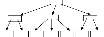
Figure 1.1 shows a very simple B-tree with a root node and four leaf
nodes. Individual records and keys within the nodes are not shown.
The leaf nodes contain records with keys in disjoint key ranges. The
root node contains pointers to the leaf nodes and separator keys that
divide the key ranges in the leaves. If the number of leaf nodes exceeds
the number of pointers and separator keys that fit in the root node,
an intermediate layer of “branch” nodes is introduced. The separator
keys in the root node divide key ranges covered by the branch nodes
(also known as internal, intermediate, or interior nodes), and separator
204

1.1 Perspectives on B-trees 205
4 leaf nodes
Root node
Fig. 1.1 A simple B-tree with root node and four leaf nodes.
keys in the branch nodes divide key ranges in the leaves. For very
large data collections, B-trees with multiple layers of branch nodes are
used. One or two branch levels are common in B-trees used as database
indexes.
Complementing this “data structures perspective” on B-trees is the
following “algorithms perspective.” Binary search in a sorted array
permits efficient search with robust performance characteristics. For
example, a search among 10
9
or 2
30
items can be accomplished with
only 30 comparisons. If the array of data items is larger than memory,
however, some form of paging is required, typically relying on virtual
memory or on a buffer pool. It is fairly inefficient with respect to I/O,
however, because for all but the last few comparisons, entire pages con-
taining tens or hundreds of keys are fetched but only a single key is
inspected. Thus, a cache might be introduced that contains the keys
most frequently used during binary searches in the large array. These
are the median key in the sorted array, the median of each resulting half
array, the median of each resulting quarter array, etc., until the cache
reaches the size of a page. In effect, the root of a B-tree is this cache,
with some flexibility added in order to enable array sizes that are not
powers of two as well as efficient insertions and deletions. If the keys
in the root page cannot divide the original large array into sub-arrays
smaller than a single page, keys of each sub-array are cached, forming
branch levels between the root page and page-sized sub-arrays.
B-tree indexes perform very well for a wide variety of operations that
are required in information retrieval and database management, even
if some other index structure is faster for some individual index opera-
tions. Perhaps the “B” in their name “B-trees” should stand for their
balanced performance across queries, updates, and utilities. Queries
include exact-match queries (“=” and “in” predicates), range queries
(“<” and “between” predicates), and full scans, with sorted output if
206 Introduction
required. Updates include insertion, deletion, modifications of existing
data associated with a specific key value, and “bulk” variants of those
operations, for example bulk loading new information and purging out-
of-date records. Utilities include creation and removal of entire indexes,
defragmentation, and consistency checks. For all of those operations,
including incremental and online variants of the utilities, B-trees also
enable efficient concurrency control and recovery.
1.2 Purpose and Scope
Many students, researchers, and professionals know the basic facts
about B-tree indexes. Basic knowledge includes their organization
in nodes including one root and many leaves, the uniform distance
between root and leaves, their logarithmic height and logarithmic
search effort, and their efficiency during insertions and deletions. This
survey briefly reviews the basics of B-tree indexes but assumes that
the reader is interested in more detailed and more complete informa-
tion about modern B-tree techniques.
Commonly held knowledge often falls short when it comes to deeper
topics such as concurrency control and recovery or to practical top-
ics such as incremental bulk loading and structural consistency check-
ing. The same is true about the many ways in which B-trees assist in
query processing, e.g., in relational databases. The goal here is to make
such knowledge readily available as a survey and as a reference for the
advanced student or professional.
The present survey goes beyond the “classic” B-tree references [7, 8,
27, 59] in multiple ways. First, more recent techniques are covered, both
research ideas and proven implementation techniques. Whereas the first
twenty years of B-tree improvements are covered in those references, the
last twenty years are not. Second, in addition to core data structure and
algorithms, the present survey also discusses their usage, for example
in query processing and in efficient update plans. Finally, auxiliary
algorithms are covered, for example defragmentation and consistency
checks.
During the time since their invention, the basic design of B-trees
has been improved upon in many ways. These improvements pertain
1.3 New Hardware 207
to additional levels in the memory hierarchy such as CPU caches, to
multi-dimensional data and multi-dimensional queries, to concurrency
control techniques such as multi-level locking and key range locking,
to utilities such as online index creation, and to many more aspects of
B-trees. Another goal here is to gather many of these improvements
and techniques in a single document.
The focus and primary context of this survey are B-tree indexes in
database management systems, primarily in relational databases. This
is reflected in many specific explanations, examples, and arguments.
Nonetheless, many of the techniques are readily applicable or at least
transferable to other possible application domains of B-trees, in par-
ticular to information retrieval [83], file systems [71], and “No SQL”
databases and key-value stores recently popularized for web services
and cloud computing [21, 29].
A survey of techniques cannot provide a comprehensive performance
evaluation or immediate implementation guidance. The reader still
must choose what techniques are required or appropriate for specific
environments and requirements. Issues to consider include the expected
data size and workload, the anticipated hardware and its memory
hierarchy, expected reliability requirements, degree of parallelism and
needs for concurrency control, the supported data model and query
patterns, etc.
1.3 New Hardware
Flash memory, flash devices, and other solid state storage technology
are about to change the memory hierarchy in computer systems in gen-
eral and in data management in particular. For example, most current
software assumes two levels in the memory hierarchy, namely RAM and
disk, whereas any further levels such as CPU caches and disk caches are
hidden by hardware and its embedded control software. Flash memory
might also remain hidden, perhaps as large and fast virtual memory
or as fast disk storage. The more likely design for databases, however,
seems to be explicit modeling of a memory hierarchy with three or
even more levels. Not only algorithms such as external merge sort but
208 Introduction
also storage structures such as B-tree indexes will need a re-design and
perhaps a re-implementation.
Among other effects, flash devices with their very fast access latency
are about to change database query processing. They likely will shift
the break-even point toward query execution plans based on index-to-
index navigation, away from large scans and large set operations such
as sort and hash join. With more index-to-index navigation, tuning the
set of indexes including automatic incremental index creation, growth,
optimization, etc. will come more into focus in future database engines.
As much as solid state storage will change tradeoffs and optimiza-
tions for data structures and access algorithms, many-core processors
will change tradeoffs and optimizations for concurrency control and
recovery. High degrees of concurrency can be enabled only by appro-
priate definitions of consistent states and of transaction boundaries,
and recovery techniques for individual transactions and for the system
state must support them. These consistent intermediate states must be
defined for each kind of index and data structure, and B-trees will likely
be first index structure for which such techniques are implemented
in production-ready database systems, file systems, and key-value
stores.
In spite of future changes for databases and indexes on flash devices
and other solid state storage technology, the present survey often men-
tions tradeoffs or design choices appropriate for traditional disk drives,
because much of the presently known and implemented techniques have
been invented and designed in this context. The goal is to provide com-
prehensive background knowledge about B-trees for those research-
ing and implementing techniques appropriate for the new types of
storage.
1.4 Overview
The next section (Section 2) sets out the basics as they may be found in
a college level text book. The following sections cover implementation
techniques for mature database management products. Their topics
are implementation techniques for data structures and algorithms
1.4 Overview 209
(Section 3), transactional techniques (Section 4), query processing
using B-trees (Section 5), utility operations specific to B-tree indexes
(Section 6), and B-trees with advanced key structures (Section 7).
These sections might be more suitable for an advanced course on data
management implementation techniques and for a professional devel-
oper desiring in-depth knowledge about B-tree indexes.

2
Basic Techniques
B-trees enable efficient retrieval of records in the native sort order
the index because, in a certain sense, B-trees capture and preserve
the result of a sort operation. Moreover, they preserve the sort effort
in a representation that can accommodate insertions, deletions, and
updates. The relationship between B-trees and sorting can be exploited
in many ways; the most common ones are that a sort operation can
be avoided if an appropriate B-tree exists and that the most effi-
cient algorithm for B-tree creation eschews random “insert” operations
and instead pays the cost of an initial sort for the benefit of efficient
“append” operations.
Figure 2.1 illustrates how a B-tree index can preserve or cache
the sort effort. With the output of a sort operation, the B-tree with
root, leaf nodes, etc. can be created very efficiently. A subsequent
scan can retrieve data sorted without additional sort effort. In addition
Sort Scan
Fig. 2.1 Caching the sort effort in a B-tree.
210
211
to preserving the sort effort over an arbitrary length of time, B-trees
also permit efficient insertions and deletions, retaining their native sort
order and enabling efficient scans in sorted order at any time.
Ordered retrieval aids many database operations, in particular sub-
sequent join and grouping operations. This is true if the list of sort keys
required in the subsequent operation is precisely equal to or a prefix of
that in the B-tree. It turns out, however, that B-trees can save a lot of sort
effort in many more cases. A later section will consider the relationship
between B-tree indexes and database query operations in detail.
B-trees share many of their characteristics with binary trees, raising
the question why binary trees are commonly used for in-memory data
structures and B-trees for on-disk data. The reason is quite simple: disk
drives have always been block-access devices, with a high overhead per
access. B-trees exploit disk pages by matching the node size to the
page size, e.g., 4 KB. In fact, B-trees on today’s high-bandwidth disks
perform best with nodes of multiple pages, e.g., 64 KB or 256 KB.
Inasmuch as main memory should be treated as a block-access device
when accessed through CPU caches and their cache lines, B-trees in
memory also make sense. Later sections will resume this discussion of
memory hierarchies and their effect on optimal data structures and
algorithm for indexes and specifically B-trees.
B-trees are more similar to 2-3-trees, in particular as both data
structures have a variable number of keys and child pointers in a node.
In fact, B-trees can be seen as a generalization of 2-3-trees. Some
books treat them both as special cases of (a, b)-trees with a ≥ 2 and
b ≥ 2a − 1 [92]. The number of child pointers in a canonical B-tree
node varies between N and 2N − 1. For a small page size and a partic-
ularly large key size, this might indeed be the range between 2 and 3.
The representation of a single node in a 2-3-tree by linking two binary
nodes also has a parallel in B-trees, discussed later as B
link
-trees.
Figure 2.2 shows a ternary node in a 2-3-tree represented by two
binary nodes, one pointing to the other half of the ternary node rather
than a child. There is only one pointer to this ternary node from a
parent node, and the node has three child pointers.
In a perfectly balanced tree such as a B-tree, it makes sense to count
the levels of nodes not from the root but from the leaves. Thus, leaves

212 Basic Techniques
from parent
three children
45 67
Fig. 2.2 A ternary node in a 2-3-tree represented with binary nodes.
are sometimes called level-0 nodes, which are children of level-1 nodes,
etc. In addition to the notion of child pointers, many family terms are
used in connection with B-trees: parent, grandparent, ancestor, descen-
dent, sibling, and cousin. Siblings are children of the same parent node.
Cousins are nodes in the same B-tree level with different parent nodes
but the same grandparent node. If the first common ancestor is a great-
grandparent, the nodes are second cousins, etc. Family analogies are not
used throughout, however. Two siblings or cousins with adjoining key
ranges are called neighbors, because there is no commonly used term
for such siblings in families. The two neighbor nodes are called left
and right neighbors; their key ranges are called the adjacent lower and
upper key ranges.
In most relational database management systems, the B-tree code
is part of the access methods module within the storage layer, which
also includes buffer pool management, lock manager, log manager, and
more. The relational layer relies on the storage layer and implements
query optimization, query execution, catalogs, and more. Sorting and
index maintenance span those two layers. For example, large updates
may use an update execution plan similar to a query execution plan
to maintain each B-tree index as efficiently as possible, but individ-
ual B-tree modifications as well as read-ahead and write-behind may
remain within the storage layer. Details of such advanced update and
prefetch strategies will be discussed later.
In summary:
•
B-trees are indexes optimized for paged environments, i.e.,
storage not supporting byte access. A B-tree node occupies a
page or a set of contiguous pages. Access to individual records
requires a buffer pool in byte-addressable storage such as
RAM.
2.1 Data Structures 213
•
B-trees are ordered; they effectively preserve the effort spent
on sorting during index creation. Differently than sorted
arrays, B-trees permit efficient insertions and deletions.
•
Nodes are leaves or branch nodes. One node is distinguished
as root node.
•
Other terms to know: parent, grandparent, ancestor, child,
descendent, sibling, cousin, neighbor.
•
Most implementations maintain the sort order within each
node, both leaf nodes and branch nodes, in order to enable
efficient binary search.
•
B-trees are balanced, with a uniform path length in root-to-
leaf searches. This guarantees uniformly efficient search.
2.1 Data Structures
In general, a B-tree has three kinds of nodes: a single root, a lot of leaf
nodes, and as many branch nodes as required to connect the root and
the leaves. The root contains at least one key and at least two child
pointers; all other nodes are at least half full at all times. Usually all
nodes have the same size, but this is not truly required.
The original design for B-trees has user data in all nodes. The design
used much more commonly today holds user data only in the leaf nodes.
The root node and the branch nodes contain only separator keys that
guide the search algorithm to the correct leaf node. These separator
keys may be equal to keys of current or former data, but the only
requirement is that they can guide the search algorithm.
This design has been called B
+
-tree but it is nowadays the default
design when B-trees are discussed. The value of this design is that dele-
tion can affect only leaf nodes, not branch nodes and that separator keys
in branch nodes can be freely chosen within the appropriate key range.
If variable-length records are supported as discussed later, the separator
keys can often be very short. Short separator keys increase the node fan-
out, i.e., the number of child pointers per node, and decrease the B-tree
height, i.e., the number of nodes visited in a root-to-leaf search.
The records in leaf nodes contain a search key plus some associated
information. This information can be all the columns associated with
214 Basic Techniques
Fig. 2.3 B-tree with root, branch nodes, and leaves.
a table in a database, it can be a pointer to a record with all those
columns, or it can be anything else. In most parts of this survey, the
nature, contents, and semantics of this information are not important
and not discussed further.
In both branch nodes and leaves, the entries are kept in sorted order.
The purpose is to enable fast search within each node, typically using
binary search. A branch node with N separator keys contains N +1
child pointers, one for each key range between neighboring separator
keys, one for the key, range below the smallest separator key, and one
for the key range above the largest separator key.
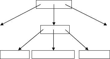
Figure 2.3 illustrates a B-tree more complex than the one in
Figure 1.1, including one level of branch nodes between the leaves and
the root. In the diagram, the root and all branch nodes have fan-outs
of 2 or 3. In a B-tree index stored on disk, the fan-out is determined
by the sizes of disk pages, child pointers, and separator keys. Keys are
omitted in Figure 2.3 and in many of the following figures unless they
are required for the discussion at hand.
Among all possible node-to-node pointers, only the child point-
ers are truly required. Many implementations also maintain neighbor
pointers, sometimes only between leaf nodes and sometimes only in one
direction. Some rare implementations have used parent pointers, too,
e.g., a Siemens product [80]. The problem with parent pointers is that
they force updates in many child nodes when a parent node is moved
or split. In a disk-based B-tree, all these pointers are represented as
page identifiers.
B-tree nodes may include many additional fields, typically in a
page header. For consistency checking, there are table or index iden-
tifier plus the B-tree level, starting with 0 for leaf pages; for space
2.2 Sizes, Tree Height, etc. 215
management, there is a record count; for space management with
variable-size records, there are slot count, byte count, and lowest record
offset; for data compression, there may be a shared key prefix including
its size plus information as required for other compression techniques;
for write-ahead logging and recovery, there usually is a Page LSN (log
sequence number) [95]; for concurrency control, in particular in shared-
memory systems, there may be information about current locks; and for
efficient key range locking, consistency checking, and page movement
as in defragmentation, there may be fence keys, i.e., copies of separator
keys in ancestor pages. Each field, its purpose, and its use are discussed
in a subsequent section.
•
Leaf nodes contain key values and some associated informa-
tion. In most B-trees, branch nodes including the root node
contain separator keys and child pointers but no associated
information.
•
Child pointers are essential. Sibling pointers are often imple-
mented but not truly required. Parent pointers are hardly
ever employed.
•
B-tree nodes usually contain a fixed-format page header, a
variable-size array of fixed-size slots, and a variable-size data
area. The header contains a slot counter, information per-
taining to compression and recovery, and more. The slots
serve space management for variable-size records.
2.2 Sizes, Tree Height, etc.
In traditional database designs, the typical size of a B-tree node is
4–8 KB. Larger B-tree nodes might seem more efficient for today’s disk
drives based on multiple analyses [57, 86] but nonetheless are rarely
used in practice. The size of a separator key can be as large as a record
but it can also be much smaller, as discussed later in the section on
prefix B-trees. Thus, the typical fan-out, i.e., the number of children
or of child pointers, is sometimes only in the tens, typically in the
hundreds, and sometimes in the thousands.
If a B-tree contains N records and L records per leaf, the B-tree
requires N/L leaf nodes. If the average number of children per parent
216 Basic Techniques
is F , the number of branch levels is log
F
(N/L). For example, the B-tree
in Figure 2.3 has 9 leaf nodes, a fan-out F = 3, and thus log
3
9=2
branch levels. Depending on the convention, the height of this B-tree
is 2 (levels above the leaves) or 3 (levels including the leaves). In order
to reflect the fact that the root node usually has a different fan-out,
this expression is rounded up. In fact, after some random insertions
and deletions, space utilization in the nodes will vary among nodes.
The average space utilization in B-trees is usually given as about 70%
[75], but various policies used in practice and discussed later may result
in higher space utilization. Our goal here is not to be precise but to
show crucial effects, basic calculations, and the orders of magnitude of
various choices and parameters.
If a single branch node can point to hundreds of children, then
the distance between root and leaves is usually very small and 99% or
more of all B-tree nodes are leaves. In other words, great-grandparents
and even more distant ancestors are rare in practice. Thus, for the
performance of random searches based on root-to-leaf B-tree traversals,
treatment of only 1% of a B-tree index and thus perhaps only 1% of
a database determine much of the performance. For example, keeping
the root of a frequently used B-tree index in memory benefits many
searches with little cost in memory or cache space.
•
The B-tree depth (nodes along a root-to-leaf path) is loga-
rithmic in the number of records. It is usually small.
•
Often more than 99% of all nodes in a B-tree are leaf nodes.
•
B-tree pages are filled between 50% and 100%, permitting
insertions and deletions as well as splitting and merging nodes.
Average utilization after random updates is about 70%.
2.3 Algorithms
The most basic, and also the most crucial, algorithm for B-trees is
search. Given a specific value for the search key of a B-tree or for a
prefix thereof, the goal is to find, correctly and as efficiently as possible,
all entries in the B-tree matching the search key. For range queries, the
search finds the lowest key satisfying the predicate.

2.3 Algorithms 217
A search requires one root-to-leaf pass. In each branch node, the
search finds the pair of neighboring separator keys smaller and larger
than the search key, and then continues by following the child pointer
between those two separator keys.
The number of comparisons during binary search among L records
in a leaf is log
2
(L), ignoring rounding effects. Similarly, binary search
among F child pointers in a branch node requires log
2
(F ) comparisons.
The number of leaf nodes in a B-tree with N records and L records
per leaf is N/L. The depth of a B-tree is log
F
(N/L), which is also the
number of branch nodes visited in a root-to-leaf search. Together, the
number of comparisons in a search inspecting both branch nodes and
a leaf node is log
F
(N/L) × log
2
(F ) + log
2
(L). By elementary rules for
algebra with logarithms, the product term simplifies to log
2
(N/L) and
then the entire expression simplifies to log
2
(N). In other words, node
size and record size may produce secondary rounding effects in this
calculation but the record count is the only primary influence on the
number of comparisons in a root-to-leaf search in a B-tree.
Figure 2.4 shows parts of a B-tree including some key values.
A search for the value 31 starts at the root. The pointer between the
key values 7 and 89 is followed to the appropriate branch node. As the
search key is larger than all keys in that node, the right-most pointer
is followed to a leaf. A search within that node determines that the
key value 31 does not exist in the B-tree. A search for key value 23
would lead to the center node in Figure 2.4, assuming a convention
that a separator key serves as inclusive upper bound for a key range.
The search cannot terminate when the value 23 is found at the branch
7 89
23
15
83
9
13
11
17
23
29
19
Fig. 2.4 B-tree with root-to-leaf search.
218 Basic Techniques
level. This is because the purpose of most B-tree searches is retrieving
the information attached to each key and information contents exists
only in leaves in most B-tree implementations. Moreover, as can be
seen for key value 15 in Figure 2.4, a key that might have existed at
some time in a valid leaf entry may continue to serve as separator key
in a nonleaf node even after the leaf entry has been removed.
An exact-match query is complete after the search, but a range
query must scan leaf nodes from the low end of the range to the high
end. The scan can employ neighbor pointers if they exist in the B-tree.
Otherwise, parent and grandparent nodes and their child pointers must
be employed. In order to exploit multiple asynchronous requests, e.g.,
for a B-tree index stored in a disk array or in network-attached stor-
age, parent and grandparent nodes are needed. Range scans relying on
neighbor pointers are limited to one asynchronous prefetch at-a-time
and therefore unsuitable for arrays of storage devices or for virtualized
storage.
Insertions start with a search for the correct leaf to place the new
record. If that leaf has the required free space, the insertion is complete.
Otherwise, a case called “overflow,” the leaf needs to be split into two
leaves and a new separator key must be inserted into the parent. If the
parent is already full, the parent is split and a separator key is inserted
into the appropriate grandparent node. If the root node needs to be
split, the B-tree grows by one more level, i.e., a new root node with two
children and only one separator key. In other words, whereas the depth
of many tree data structures grows at the leaves, the depth of B-trees
grows at the root. This is what guarantees perfect balance in a B-tree.
At the leaf level, B-trees grow only in width, enabled by the variable
number of child nodes in each parent node. In some implementations
of B-trees, the old root page becomes the new root page and the old
root contents are distributed into the two newly allocated nodes. This
is a valuable technique if modifying the page identifier of the root node
in the database catalogs is expensive or if the page identifier is cached
in compiled query execution plans.
Figure 2.5 shows the B-tree of Figure 2.4 after insertion of the key 22
and a resulting leaf split. Note that the separator key propagated to
the parent node can be chosen freely; any key value that separates the

2.3 Algorithms 219
20
7 89
23
15
83
9
13
11 17
23
29
19 22
Fig. 2.5 B-tree with insertion and leaf split.
two nodes resulting from the split is acceptable. This is particularly
useful for variable-length keys: the shortest possible separator key can
be employed in order to reduce space requirements in the parent node.
Some implementations of B-trees delay splits as much as possible,
for example by load balancing among siblings such that a full node can
make space for an insertion. This design raises the code complexity but
also the space utilization. High space utilization enables high scan rates
if data transfer from storage devices is the bottleneck. Moreover, splits
and new page allocations may force additional seek operations during
a scan that are expensive in disk-based B-trees.
Deletions also start with a search for the correct leaf that contains
the appropriate record. If that leaf ends up less than half full, a case
called “underflow,” either load balancing or merging with a sibling
node can ensure the traditional B-tree invariant that all nodes other
than the root be at least half full. Merging two sibling nodes may result
in underflow in their parent node. If the only two children of the root
node merge, the resulting node becomes the root and the old root is
removed. In other words, the depth of B-trees both grows and shrinks at
the root. If the page identifier of the root node is cached as mentioned
earlier, it might be practical to move all contents to the root node and
de-allocate the two children of the root node.
Figure 2.6 shows the B-tree from Figure 2.5 after deletion of key
value 23. Due to underflow, two leaves were merged. Note that the
separator key 23 was not removed because it still serves the required
function.
Many implementations, however, avoid the complexities of load
balancing and of merging and simply let underflows persist.
A subsequent insertion or defragmentation will presumably resolve
220 Basic Techniques
7 89
23
15
83
9
13
11 17
29
19 22
Fig. 2.6 Deletion with load balancing.
it later. A recent study of worst case and average case behaviors of
B-trees concludes that “adding periodic rebuilding of the tree,... the
data structure... istheoretically superior to standard B
+
-trees in many
ways [and]... rebalancing on deletion can be considered harmful” [116].
Updates of key fields in B-tree records often require deletion in one
place and insertion in another place in the B-tree. Updates of nonkey
fixed-length fields happen in place. If records contain variable-length
fields, a change in the record size might force overflow or underflow
similar to insertion or deletion.
The final basic B-tree algorithm is B-tree creation. Actually, there
are two algorithms, characterized by random insertions and by prior
sorting. Some database products used random insertions in their initial
releases but their customers found creation of large indexes very slow.
Sorting the future index entries prior to B-tree creation permits many
efficiency gains, from massive I/O savings to various techniques saving
CPU effort. As the future index grows larger than the available buffer
pool, more and more insertions require reading, updating, and writing a
page. A database system might also require logging each such change in
the recovery log, whereas most systems nowadays employ non-logged
index creation, which is discussed later. Finally, a stream of append
operations also encourages a B-tree layout on disk that permits efficient
scans with a minimal number of disk seeks. Efficient sort algorithms
for database systems have been discussed elsewhere [46].
•
If binary search is employed in each node, the number of
comparisons in a search is independent of record and node
sizes except for rounding effects.
2.4 B-trees in Databases 221
•
B-trees support both equality (exact-match) predicates and
range predicate. Ordered scans can exploit neighbor pointers
or ancestor nodes for deep (multi-page) read-ahead.
•
Insertions use existing free space or split a full node into two
half-full nodes. A split requires adding a separator key and
a child pointer to the parent node. If the root node splits, a
new root node is required and the B-tree grows by one level.
•
Deletions may merge half-full nodes. Many implementations
ignore this case and rely on subsequent insertions or defrag-
mentation (reorganization) of the B-tree.
•
Loading B-trees by repeated random insertion is very slow;
sorting future B-tree entries permits efficient index creation.
2.4 B-trees in Databases
Having reviewed the basics of B-trees as a data structure, it is also
required to review the basics of B-trees as indexes, for example in
database systems, where B-tree indexes have been essential and ubiq-
uitous for decades. Recent developments in database query processing
have focused on improvements of large scans, e.g., by sharing scans
among concurrent queries [33, 132], by a columnar data layout that
reduces the scan volume in many queries [17, 121], or by predicate
evaluation by special hardware, such as FPGAs. The advent of flash
devices in database servers will likely result in more index usage in
database query processing — their fast access times encourage small
random accesses whereas traditional disk drives with high capacity and
high bandwidth favor large sequential accesses. With the B-tree index
the default choice in most systems, the various roles and usage patterns
of B-tree indexes in databases deserve attention. We focus here on rela-
tional databases because their conceptual model is fairly close to the
records and fields used in the storage layer of all database systems as
well as other storage services.
In a relational database, all data is logically organized in tables
with columns identified by name and rows identified by unique values
in columns forming the table’s primary key. Relationships among tables
are captured in foreign key constraints. Relationships among rows are

222 Basic Techniques
expressed in foreign key columns, which contain copies of primary key
values elsewhere. Other forms of integrity constraints include unique-
ness of one or more columns; uniqueness constraints are often enforced
using a B-tree index.
The simplest representation for a database table is a heap, a col-
lection of pages holding records in no particular order, although often
in the order of insertion. Individual records are identified and located
by means of page identifier and slot number (see below in Section 3.3),
where the page identifier may include a device identifier. When a record
grows due to an update, it might need to move to a new page. In that
case, either the original location retains “forwarding” information or
all references to the old location, e.g., in indexes, must be updated. In
the former case, all future accesses incur additional overhead, possibly
the cost of a disk read; in the latter case, a seemingly simple change
may incur a substantial unforeseen and unpredictable cost.
Figure 2.7 shows records (solid lines) and pages (dashed lines)
within a heap file. Records are of variable size. Modifications of two
records have changed their sizes and forced moving the record contents
to another page with forwarding pointers (dotted lines) left behind in
the original locations. If an index points to records in this file, forward-
ing does not affect the index contents but does affect the access times
in subsequent queries.
If a B-tree structure rather than a heap is employed to store all
columns in a table, it is called a primary index here. Other commonly
used names include clustered index or index-organized table. In a sec-
ondary index, also commonly called a non-clustered index, each entry
must contain a reference to a row or a record in the primary index.
This reference can be a search key in a primary index or it can be a
record identifier including a page identifier. The term “reference” will
often be used below to refer to either one. References to records in a
primary index are also called bookmarks in some contexts.
Fig. 2.7 Heap file with variable-length records and forwarding pointers.

2.4 B-trees in Databases 223
Secondary
index
Primary
index
Query search
key
Primary
search key
Fig. 2.8 Index navigation with a search key.
Both designs, reference by search key and reference by record identi-
fier, have advantages and disadvantages [68]; there is no perfect design.
The former design requires a root-to-leaf search in the primary index
after each search in the secondary index. Figure 2.8 illustrates the dou-
ble index search when the primary data structure for a table is a pri-
mary index and references in secondary indexes use search keys in the
primary index. The search key extracted from the query requires an
index search and root-to-leaf traversal in the secondary index. The
information associated with a key in the secondary index is a search
key for the primary index. Thus, after a successful search in the sec-
ondary index, another B-tree search is required in the primary index
including a root-to-leaf traversal there.
The latter design permits faster access to records in the primary
index after a search in the secondary index. When a leaf in the pri-
mary index splits, however, this design requires many updates in all
relevant secondary indexes. These updates are expensive with many
I/O operations and B-tree searches, they are infrequent enough to be
always surprising, they are frequent enough to be disruptive, and they
impose a substantial penalty due to concurrency control and logging
for these updates.
A combination is also possible, with the page identifier as a hint
and the search key as the fall-back. This design has some intrinsic
difficulties, e.g., when a referenced page is de-allocated and later re-
allocated for a different data structure. Finally, some systems employ
clustering indexes over heap files; their goal is to keep the heap file
sorted if possible but nonetheless enable fast record access via record
identifiers.
224 Basic Techniques
In databases, all B-tree keys must be unique, even if the user-defined
B-tree key columns are not. In a primary index, unique keys are required
for correct retrieval. For example, each reference found in a secondary
index must guide a query to exactly one record in the primary index —
therefore, the search keys in the primary index must be unambiguous in
the reference-by-search-key design. If the user-defined search key for a pri-
mary index is a person’s last name, values such as “Smith” are unlikely to
safely identify individual records in the primary index.
In a secondary index, unique keys are required for correct deletion.
Otherwise, deletion of a logical row and its record in a primary index
might be followed by deletion of the wrong entry in a non-unique sec-
ondary index. For example, if the user-defined search in a secondary
index is a person’s first name, deletion of a record in the primary index
containing “Bob Smith” must delete only the correct matching record
in the secondary index, not all records with search key “Bob” or a
random such record.
If the search key specified during index creation is unique due to
uniqueness constraints, the user-defined search key is sufficient. Of
course, once a logical integrity constraint is relied upon in an index
structure, dropping the integrity constraint must be prevented or fol-
lowed by index reorganization. Otherwise, some artificial field must be
added to the user-defined index key. For primary indexes, some systems
employ a globally unique “database key” such as a microsecond times-
tamp, some use an integer value unique within the table, and some use
an integer value unique among B-tree entries with the same value in
the user-defined index key. For secondary indexes, most systems simply
add the reference to the search key of the primary index.
B-tree entries are kept sorted on their entire unique key. In a primary
index, this aids efficient retrieval; in a secondary index, it aids efficient
deletion. Moreover, the sorted lists of references for each unique search
key enable efficient list intersection and union. For example, for a query
predicate “A = 5 and B = 15,” sorted lists of references can be obtained
from indexes on columns A and B and their intersection computed by
a simple merge algorithm.
The relationships between tables and indexes need not be as tight
and simple as discussed so far. A table may have calculated columns
2.4 B-trees in Databases 225
that are not stored at all, e.g., the difference (interval) between two date
(timestamp) columns. On the other hand, a secondary index might
be organized on such a column, and in this case necessarily store a
copy of the column. An index might even include calculated columns
that effectively copy values from another table, e.g., the table of order
details might include a customer identifier (from the table of orders)
or a customer name (from the table of customers), if the appropriate
functional dependencies and foreign key constraints are in place.
Another relationship that is usually fixed, but need not be, is the
relationship between uniqueness constraints and indexes. Many systems
automatically create an index when a uniqueness constraint is defined
and drop the index when the constraint is dropped. Older systems did
not support uniqueness constraints at all but only unique indexes. The
index is created even if an index on the same column set already exists,
and the index is dropped even if it would be useful in future queries. An
alternative design merely requires that some index with the appropriate
column set exists while a uniqueness constraint is active. For instant
definition of a uniqueness constraint with existing useful index, a possi-
ble design counts the number of unique keys during each insertion and
deletion in any index. In a sorted index such as a B-tree, a count should
be maintained for each key prefix, i.e., for the first key field only, the
first and second key fields together, etc. The required comparisons are
practically free as they are a necessary part of searching for the correct
insertion or deletion point. A new uniqueness constraint is instantly
verified if the count of unique key values is equal to the record count
in the index.
Finally, tables and indexes might be partitioned horizontally (into
sets of rows) or vertically (into sets of columns), as will be discussed
later. Partitions usually are disjoint but this is not truly required. Hor-
izontal partitioning can be applied to a table such that all indexes of
that table follow the same partitioning rule, sometimes called “local
indexes.” Alternatively, partitioning can be applied to each index indi-
vidually, with secondary indexes partitioned with their own partition-
ing rule different from the primary index, which is sometimes called
“global indexes.” In general, physical database design or the separation
226 Basic Techniques
of logical tables and physical indexes remains an area of opportunity
and innovation.
•
B-trees are ubiquitous in databases and information retrieval.
•
If multiple B-trees are related, e.g., the primary index and the
secondary index of a database table, pointers can be physi-
cal addresses (record identifiers) or logical references (search
keys in the primary index). Neither choice is perfect, both
choices have been used.
•
B-tree entries must be unique in order to ensure correct
updates and deletions. Various mechanisms exist to force
uniqueness by adding an artificial key value.
•
Traditional database design rigidly connects tables and
B-trees, much more rigidly then truly required.
2.5 B-trees Versus Hash Indexes
It might seem surprising that B-tree indexes have become ubiquitous
whereas hash indexes have not, at least not in database systems.
Two arguments seem to strongly favor hash indexes. First, hash
indexes should save I/O costs due to a single I/O per look-up, whereas
B-trees require a complete root-to-leaf traversal for each search.
Second, hash indexes and hash values should also save CPU effort
due to efficient comparisons and address calculations. Both of these
arguments have only very limited validity, however, as explained in the
following paragraphs. Moreover, B-trees have substantial advantages
over hash indexes with respect to index creation, range predicates,
sorted retrieval, phantom protection in concurrency control, and more.
These advantages, too, are discussed in the following paragraphs. All
techniques mentioned here are explained in more depth in subsequent
sections.
With respect to I/O savings, it turns out that fairly simple imple-
mentation techniques can render B-tree indexes competitive with hash
indexes in this regard. Most B-trees have a fan-out of 100s or 1,000s.
For example, for node of 8 KB and records of 20 bytes, 70% utiliza-
tion means 140 child nodes per parent node. For larger node sizes

2.5 B-trees Versus Hash Indexes 227
(say 64 KB), good defragmentation (enabling run-length encoding of
child pointers, say 2 bytes on average), key compression using prefix
and suffix truncation (say 4 bytes on average per entry), 70% utilization
means 5,600 child nodes per parent node. Thus, root-to-leaf paths are
short and more than 99% or even 99.9% of pages in a B-tree are leaf
nodes. These considerations must be combined with the traditional
rule that many database servers run with memory size equal to 1–
3% of storage size. Today and in the future, the percentage might be
higher, up to 100% for in-memory databases. In other words, for any
B-tree index that is “warm” in the buffer pool, all branch nodes will be
present in the buffer pool. Thus, each B-tree search only requires a sin-
gle I/O, the leaf page. Moreover, the branch nodes could be fetched into
the buffer pool in preparation of repeated look-up operations, perhaps
even pinned in the buffer pool. If they are pinned, further optimizations
could be applied, e.g., spreading separator keys into a separate array
such that interpolation search is most effective, replacing or augment-
ing child pointers in form of page identifiers with child pointers in form
of memory pointers, etc.
Figure 2.9 illustrates the argument. All B-tree levels but the leaf
nodes easily fit into the buffer pool in RAM memory. For leaf pages,
a buffer pool might employ the least-recently-used (LRU) replacement
policy. Thus, for searches with random search keys, only a single I/O
operation is required, similar to a hash index if one is available in a
database system.
With respect to CPU savings, B-tree indexes can compete with hash
indexes using a few simple implementation techniques. B-tree indexes
support a wide variety of search keys, but they also support very simple
Root to parents-
of-leaves
< 1% of B-tree
B-tree leaves
>99% of B-
tree pages
I/O required
7 89
23
15
83
9
13
11 17
29
19 22
Fig. 2.9 B-tree levels and buffering.
228 Basic Techniques
ones such as hash values. Where hash indexes can be used, a B-tree on
hash values will also provide sufficient functionality. In other cases, a
“poor man’s normalized key” can be employed and even be sufficient,
rendering all additional comparison effort unnecessary. Later sections
discuss normalized keys, poor man’s normalized keys, and caching poor
man’s normalized keys in the “indirection vector” that is required for
variable-size records. In sum, poor man’s normalized keys and the indi-
rection vector can behave similarly to hash values and hash buckets.
B-trees also permit direct address calculation. Specifically, inter-
polation search may guide the search faster than binary search. A
later section discusses interpolation search including avoiding worst-
case behavior of pure interpolation by switching to binary search after
two interpolation steps, and more.
While B-tree indexes can be competitive with hash indexes based on
a few implementation techniques, B-trees also have distinct advantages
over hash indexes. For example, space management in B-trees is very
straightforward. In the simplest implementations, full nodes are split
into two halves and empty nodes are removed. Multiple schemes have
been invented for hash indexes to grow gracefully, but none seems quite
as simple and robust. Algorithms for graceful shrinking of hash indexes
are not widely known.
Probably the strongest arguments for B-trees over hash indexes
pertain to multi-field indexes and to nonuniform distributions of key
values. A hash index on multiple fields requires search keys for all those
fields such that a hash value can be calculated. A B-tree index, on the
other hand, can efficiently support exact-match queries for a prefix of
the index key, i.e., any number of leading index fields. In this way, a
B-tree with N search keys can be as useful as N hash indexes. In fact,
B-tree indexes can support many other forms of queries; it is not even
required that the restricted fields are leading fields in the B-tree’s sort
order [82].
With respect to nonuniform (“skewed”) distributions of key values,
imagine a table with 10
9
rows that needs a secondary index on a col-
umn with the same value in 10% of the rows. A hash index requires
introduction of overflow pages, with additional code for index creation,
insertion, search, concurrency control, recovery, consistency checks, etc.
2.5 B-trees Versus Hash Indexes 229
For example, when a row in the table is deleted, an expensive search is
required before the correct entry in the secondary index can be found
and removed, whereupon overflow pages might need to be merged. In a
B-tree, entries are always unique, if necessary by appending a field to
the search key as discussed earlier. In hash indexes, the additional code
requires additional execution time as well as additional effort for testing
and maintenance. Due to the well-defined sort order in B-trees, neither
special code nor extra time is required in any of the index functions.
Another strong argument in favor of B-trees is index creation. After
extracting future index entries and sorting them, B-tree creation is sim-
ple and very efficient, even for the largest data collections. An efficient,
general-purpose sorting algorithm is readily available in most systems
managing large data. Equally efficient index creation for hash indexes
would require a special-purpose algorithm, if it is possible at all. Index
creation by repeated random insertions is extremely inefficient for both
B-trees and hash indexes. Techniques for online index creation (with
concurrent database updates) are well known and widely implemented
for B-trees but not for hash indexes.
An obvious advantage of B-trees over hash indexes is the support for
ordered scans and for range predicates. Ordered scans are important for
key columns and set operations such as merge join and grouping; range
predicates are usually more important for nonkey columns. In other
words, B-trees are superior to hash indexes for both key columns and
nonkey columns in relational databases, also known as dimensions and
measures in online analytical processing. Ordering also has advantages
for concurrency control, in particular phantom protection by means
of key range locking (covered in detail later) rather than locking key
values only.
Taken together, these arguments favor B-trees over hash indexes
as a general indexing technique for databases and many other data
collections. Where hash indexes seem to have an advantage, appropriate
B-tree implementation techniques minimize it. Thus, very few database
implementation teams find hash indexes among the opportunities or
features with a high ratio of benefit and effort, in particular if B-tree
indexes are required in any case in order to support range queries and
ordered scans.
230 Basic Techniques
While nodes of 10 KB likely result in B-trees with multiple levels
of branch nodes, nodes of 1 MB probably do not. In other words, the
considerations above may apply to B-tree indexes on flash storage but
probably not on disks. For disks, it is probably best to cache all branch
nodes in memory and to employ fairly small leaf nodes such that neither
transfer bandwidth nor buffer space is wasted on unwanted records.
•
B-tree indexes are ubiquitous, whereas hash indexes are not,
even though hash indexes promise exact-match look-up with
direct address calculation in the hash directory and a single
I/O.
•
B-tree software can provide similar benefits if desired. In
addition, B-trees support efficient index creation based on
sorting, support for exact match predicates and for partial
predicates, graceful degradation in case of duplicate or dis-
tribution skew among the key values, and ordered scans.
2.6 Summary
In summary of this section on the basic data structure, B-trees are
ordered, balanced search trees optimized for block-access devices such
as disks. They guarantee good performance for various types of searches
well as for insertions, deletions, and updates. Thus, they are particu-
larly suitable to databases and in fact have been ubiquitous in databases
for decades.
Over time, many techniques have been invented and implemented
beyond the basic algorithms and data structures. These practical
improvements are covered in the next few sections.

3
Data Structures and Algorithms
The present section focuses on data structures and algorithms found in
mature data management systems but usually not in college-level text
books; the subsequent sections cover transactional techniques, B-trees
and their usage in database query processing, and B-tree utilities.
While only a single sub-section below is named “data compression,”
almost all sub-sections pertain to compression in some form: storing
fewer bytes per record, describing multiple records together, comparing
fewer bytes in each search, modifying fewer bytes in each update, and
avoiding fragmentation and wasted space. Efficiency in space and time
is the theme of this section.
The following sub-sections are organized such that the first group
pertains to the size and internal structure of nodes, the next group
to compression specific to B-trees, and the last group to management
of free space. Most of the techniques in the individual sub-sections
are independent of others, although certain combinations may ease
their implementation. For example, prefix- and suffix-truncation require
detailed and perhaps excessive record keeping unless key values are nor-
malized into binary strings.
231
232 Data Structures and Algorithms
3.1 Node Size
Even the earliest papers on B-trees discussed the optimal node size
for B-trees on disk [7]. It is governed primarily by access latency and
transfer bandwidth as well as the record size. High latency and high
bandwidth both increase the optimal node size; therefore, the optimal
node size for modern disks approaches 1 MB and the optimal on flash
devices is just a few KB [50]. A node size with equal access latency
and transfer time is a promising heuristic — it guarantees a sustained
transfer bandwidth at least half of the theoretical optimum as well as
an I/O rate at least half of the theoretical optimum. It is calculated by
multiplying access latency and transfer bandwidth. For example, for a
disk with 5 ms access latency and 200 MB/s transfer bandwidth, this
leads to 1 MB. An estimated access latency of 0.1 ms and a transfer
bandwidth of 100 MB/s lead to 10 KB as a promising node size for
B-trees on flash devices.
For a more precise optimization, the goal is maximize the number
of comparisons per unit of I/O time. Examples for this calculation can
already be found in the original B-tree papers [7]. This optimization
assumes that the goal is to optimize root-to-leaf searches and not large
range scans, I/O time and not CPU effort is the bottleneck, binary
search is used within nodes, and a fixed total number of comparisons
in a root-to-leaf B-tree search independent of the node size as discussed
above.
Figure 3.1 shows a calculation similar to those in [57]. It assumes
pages filled to 70% with records of 20 bytes, typical in secondary
indexes. For example, in a page of 4 KB holding 143 records, binary
Page size
[KB]
Records
/ page
Node
utility
I/O time
[ms]
Utility
/ time
4 143 7.163 5.020 1.427
16 573 9.163 5.080 1.804
64 2,294 11.163 5.320 2.098
128 4,588 12.163 5.640 2.157
256 9,175 13.163 6.280 2.096
1,024 36,700 15.163 10.120 1.498
4,096 146,801 17.163 25.480 0.674
Fig. 3.1 Utility for pages sizes one a traditional disk.

3.2 Interpolation Search 233
search performs a little over 7 comparisons on average. The number of
comparisons is termed the utility of the node with respect to searching
the index. I/O times in Figure 3.1 are calculated assuming 5 ms access
time and 200 MB/s (burst) transfer bandwidth. The heuristic above
would suggest a page size of 5 ms × 200 MB/s = 1,000 KB. B-tree
nodes of 128 KB enable the most comparisons (in binary search) rela-
tive to the disk device time. Historically common disk pages of 4 KB
are far from optimal for B-tree indexes on traditional disk drives. Dif-
ferent record sizes and different devices will result in different optimal
page sizes for B-tree indexes. Most importantly, devices based on flash
devices may achieve 100 times faster access times without substantially
different transfer bandwidth. Optimal B-tree node sizes will be much
smaller, e.g., 2 KB [50].
•
The node size should be optimized based on latency and
bandwidth of the underlying storage. For example, the opti-
mal page size differs for traditional disks and semiconductor
storage.
3.2 Interpolation Search
1
Like binary search, interpolation search employs the concept of a
remaining search interval, initially comprising the entire page. Instead
of inspecting the key in the center of the remaining interval like
binary search, interpolation search estimates the position of the sought
key value, typically using a linear interpolation based on the lowest
and highest key value in the remaining interval. For some keys, e.g.,
artificial identifier values generated by a sequential process such as
invoice numbers in a business operation, interpolation search works
extremely well.
In the best case, interpolation search is practically unbeatable. Con-
sider an index on the column Order-Number in the table Orders given
that order numbers and invoice numbers are assigned sequentially. Since
each order number exists precisely once, interpolation among hundreds
1
Much of this section is derived from [45].

234 Data Structures and Algorithms
or even thousands of records within a B-tree node instantly guides the
search to the correct record.
In the worst case, however, the performance of pure interpolation
search equals that of linear search due to a nonuniform distribution
of key values. The theoretical complexity is O (log log N) for search
among N keys [36, 107], or 2 to 4 steps for practical page sizes. Thus,
if the sought key has not yet been found after 3 or 4 steps, the actual
key distribution is not uniform and it might be best to perform the
remaining search using binary search.
Rather than switching from pure interpolation search to pure binary
search, a gradual transition may pay off. If interpolation search has
guided the search to one end of the remaining interval but not directly
to the sought key value, the interval remaining for binary search may
be very small or very large. Thus, it seems advisable to bias the last
interpolation step in such a way to make it very likely that the sought
key is in the smaller remaining interval.
The initial interpolation calculation might use the lowest and high-
est possible values in a page, the lowest and highest actual values,
or a regression line based on all current values. The latter technique
may be augmented with a correlation calculation that guides the initial
search steps toward interpolation or binary search. Sums and counts
required to quickly derive regression and correlation coefficients can eas-
ily be maintained incrementally during updates of individual records
in a page.
Figure 3.2 shows two B-tree nodes and their key values. In the upper
one, the correlation between slot numbers and key values is very high
(>0.998). Slope and intercept are 3.1 and 5.9, respectively (slot num-
bers start with 0). An interpolation search for key value 12 immediately
probes slot number (12 − 5.9) ÷ 3.1 = 2 (rounded), which is where key
5, 9, 12, 16, 19, 21, 25, 27, 31, 34, 36
5, 6, 15, 15, 16, 43, 95, 96, 97, 128, 499
Fig. 3.2 Sample key values.
3.3 Variable-length Records 235
value 12 indeed can be found. In other words, if the correlation between
position and key value is very strong, interpolation search is promising.
In the lower B-tree node shown in Figure 3.2, slope and intercept are
−64 and 31, respectively. More importantly, the correlation coefficient
is much lower (<0.75). Not surprisingly, interpolation search for key
value 97 starts probing at slot (97 − 64) ÷ 31 = 5 whereas the cor-
rect slot number of key value 97 is 8. Thus, if the correlation between
position and key value is weak, binary search is the more promising
approach.
•
If the key value distribution within a page is close to uniform,
interpolation search requires fewer comparisons and incurs
fewer cache faults than binary search. Artificial identifiers
such as order numbers are ideal cases for interpolation search.
•
For cases on non-uniform key value distributions, various
techniques can prevent repeated erroneous interpolation.
3.3 Variable-length Records
While B-trees are usually explained for fixed-length records in the
leaves and fixed-length separator keys in the branch nodes, B-trees
in practically all database systems support variable-length records and
variable-length separator keys. Thus, space management within B-tree
nodes is not trivial.
The standard design for variable-length records in fixed-length
pages, both in B-trees and in heap files, employs an indirection vector
(also known as slot array) with entries of fixed size. Each entry rep-
resents one record. An entry must contain the byte offset of the
record and may contain additional information, e.g., the size of the
record.
Figure 3.3 shows the most important parts of a disk page in a
database. The page header, shown far left within the page, contains
index identifier, B-tree level (for consistency checks), record count, etc.
This is followed in Figure 3.3 by the indirection vector. In heap files,
slots remain unused after a record deletion in order to ensure that
the remaining valid records retain their record identifier. In B-trees,

236 Data Structures and Algorithms
Fig. 3.3 A database page with page header, indirection vector, and variable-length records.
insertions or deletions require shifting some slot entries in order to
ensure that binary search can work correctly. (Figure 4.7 in Section 4.2
shows an alternative to this traditional design with less shifting due to
intentional gaps in the sequence of records.) Each used slot contains a
pointer (in form of a byte offset within the page) to a record. In the
diagram, the indirection vector grows from left to right and the set of
records grows from right to left. The opposite design is also possible.
Letting two data structures grow toward each other enables equally
well many small records or fewer large records.
For efficient binary search, the entries in the indirection vector are
sorted on their search key. It is not required that the entries be sorted on
their offsets, i.e., the placement of records. For example, the sequence
of slots in the left half of Figure 3.3 differs from the sequence of records
in the right half. A sort order on offsets is needed only temporarily
for consistency checks and for compaction or free space consolidation,
which may be invoked by a record insertion, by a size-changing record
update, or by a defragmentation utility.
Record insertion requires free space both for the record and for the
entry in the indirection vector. In the standard design, the indirection
vector grows from one end of the page and the data space occupied by
records grows from the opposite end. Free space for the record is usually
found very quickly by growing the data space into the free space in the
middle. Free space for the entry requires finding the correct placement
in the sorted indirection vector and then shifting entries as appropriate.
On average, half of the indirection must shift by one position.
Record deletion is fast as it typically just leaves a gap in the
data space. However, it must keep the indirection vector dense and
sorted, and thus requires shifting just like insertion. Some recent designs
require less shifting [12]. Some designs also separate separator keys
and child pointers in branch nodes in order to achieve more effective

3.4 Normalized Keys 237
compression as well as more efficient search within each branch node.
Those techniques are also discussed below.
•
Variable-size records can be supported efficiently by a level
of indirection within a page.
•
Shift operations in the indirection vector can be minimized
by gaps (invalid entries).
3.4 Normalized Keys
In order to reduce the cost of comparisons, many implementations of
B-trees transform keys into a binary string such that simply binary
comparisons suffice to sort the records during index creation and to
guide a search in the B-tree to the correct record. The key sequence
for the sort order of the original key and for the binary string are the
same, and all comparisons equivalent. This binary string may encode
multiple columns, their sort direction (e.g., descending) and collation
including local characters (e.g., case-insensitive German), string length
or string termination, etc.
Key normalization is a very old technique. It is already mentioned
by Singleton [118] without citation, presumably because it seemed a
well-known or trivial concept: “integer comparisons were used to order
normalized floating-point numbers.”
Figure 3.4 illustrates the idea based on an integer column followed
by two string columns. The initial single bit (shown underlined) indi-
cates whether the leading key column contains a valid value. Using 0
for null values and 1 for other values ensures that a null value “sorts
lower” than all other values. If the integer column value is not null, it
is stored in the next 32 bits. Signed integers require reversing some
bits to ensure the proper sort order, just like floating point values
Integer First string Second string Normalized key
2 “flow” “error” 1
0…0 0000 0000 0010 1 flow\0 1 error\0
3 “flower” “rare” 1
0…0 0000 0000 0011 1 flower\0 1 rare\0
1024 Null “brush” 1
0…0 0100 0000 0000 0 1 brush\0
Null “” Null 0
1 \0 0
Fig. 3.4 Normalized keys.
238 Data Structures and Algorithms
require proper treatment of exponent, mantissa, and the two sign bits.
Figure 3.4 assumes that the first column is unsigned. The following
single bit (also shown underlined) indicates whether the first string col-
umn contains a valid value. This value is shown here as text but really
ought to be stored in a binary format as appropriate for the desired
international collation sequence. A string termination symbol (shown
as \0) marks the end of the string. A termination symbol is required
to ensure the proper sort order. A length indicator, for example, would
destroy the main value of normalized keys, namely sorting with simple
binary comparisons. If the string termination symbol can occur as a
valid character in some strings, the binary representation must offer
one more symbol than the alphabet contains. Notice the difference in
representations between a missing value in a string column (in the third
row) and an empty string (in the fourth row).
For some collation sequences, “normalized keys” lose information.
A typical example is a language with lower and upper case letters sorted
and indexed in a case-insensitive order. In that case, two different orig-
inal strings might map to the same normalized key, and it is impossible
from the normalized key to decide which original style was used. One
solution for this problem is to store both the normalized key and the
original string value. A second solution is to append to the normal-
ized key the minimal information that enables a precise recovery of the
original writing style. A third solution, specific to B-tree indexes, is to
employ normalized keys only in branch nodes; recall that key values in
branch nodes merely guide the search to the correct child but do not
contain user data.
In many operating systems, appropriate functions are provided to
compute a normalized key from a localized string value, date value,
or time value. This functionality is used, for example, to list files in a
directory as appropriate for the local language. Adding normalization
for numeric data types is relatively straightforward, as is concatenation
of multiple normalized values. Database code must not rely on such
operating system code, however. The problem with relying on operat-
ing systems support for database indexes is the update frequency. An
operating system might update its normalization code due to an error
or extension in the code or in the definition of a local sort order; it is
3.5 Prefix B-trees 239
unacceptable, however, if such an update silently renders existing large
database indexes incorrect.
Another issue with normalized keys is that they tend to be longer
than the original string values, in particular for some languages and
their complex rules for order, sorting, and index look-up. Compres-
sion of normalized keys seems quite possible but a detailed description
seems to be missing yet in the literature. Thus, normalized keys are
currently used primarily in internal B-tree nodes, where they simplify
the implementation of prefix and suffix truncation but never require
recovery of original key values.
•
Normalized keys enable comparisons by traditional hardware
instructions, much faster than column-by-column interpola-
tion of metadata about international sort order, ascending
versus descending sort order, etc.
•
Normalized keys can be longer than a traditional represen-
tation but are amenable to compression.
•
Some systems employ normalized keys in branch nodes but
not in leaf nodes.
3.5 Prefix B-trees
Once keys have been normalized into a simple binary string, another B-
tree optimization becomes much easier to implement, namely prefix and
suffix truncation or compression [10]. Without key normalization, these
techniques would require a fair bit of bookkeeping, even if they were
applied only to entire key fields rather than to individual bytes; with
key normalization, their implementation is relatively straightforward.
Prefix truncation analyzes the keys in a B-tree node and stores
the common prefix only once, truncating it from all keys stored in the
node. Saving storage space permits increasing the number of records per
leaf and increasing the fan-out of branch nodes. In addition, the trun-
cated key bytes do not need to be considered in comparisons during a
search.
Figure 3.5 shows the same records within a B-tree node represented
without and with prefix truncation. It is immediately obvious that the
latter representation is more efficient. It is possible to combine prefix

240 Data Structures and Algorithms
Smith, Jack – 02/29/1924
Smith, Jane – 08/14/1928
Smith, Jason – 06/29/1987
Smith, Jeremy – 03/01/1983
Smith, Jill – 12/31/1956
Smith, John – 10/12/1958
…
Smith, June – 05/05/1903
Prefix = Smith, J
ack – 02/29/1924
ane – 08/14/1928
ason – 06/29/1987
eremy – 03/01/1983
ill – 12/31/1956
ohn – 10/12/1958
…
une – 05/05/1903
Fig. 3.5 A B-tree node without and with prefix truncation.
truncation with some additional compression technique, e.g., to elimi-
nate symbols from the birthdates given. Of course, it is always required
to weigh gains in run-time performance and storage efficiency against
implementation complexity including testing effort.
Prefix truncation can be applied to entire nodes or to some subset of
the keys within a node. Code simplicity argues for truncating the same
prefix from all entries in a B-tree node. Moreover, one can apply prefix
truncation based on the actual keys currently held in a node or based
on the possible key range as defined by the separator keys in parent
(and possibly other ancestor) pages. Code simplicity, in particular for
insertions, argues for prefix truncation based on the maximal possible
key range, even if prefix truncation based on actual keys might produce
better compression [87]. If prefix truncation is based on actual keys,
insertion of a new key might force reformatting all existing keys. In an
extreme case, a new record might be much smaller than the free space
in a B-tree page yet its insertion might force a page split.
The maximal possible key range for a B-tree page can be captured
by retaining two fence keys in each node, i.e., copies of separator
keys posted in parent nodes while splitting nodes. Figure 4.11 (in
Section 4.4) illustrates fence keys in multiple nodes in a B-tree index.
Fence keys have multiple benefits in B-tree implementations, e.g., for
key range locking. With respect to prefix truncation, the leading bytes
shared by the two fence keys of a page define the bytes by all current
and future key values in the page. At the same time, prefix trunca-
tion reduces the overhead imposed by fence keys, and suffix truncation
3.5 Prefix B-trees 241
(applied when leaf nodes are split) ensures that separator keys and thus
fence keys are always as short as possible.
Prefix truncation interacts with interpolation search. In particu-
lar, if the interpolation calculation uses fixed and limited precision,
truncating common prefixes enables more accurate interpolation. Thus,
normalized keys, prefix truncation, suffix truncation, and interpolation
search are a likely combination in an implementation.
A very different approach to prefix truncation technique is offset-
value coding [28]. It is used in high-performance implementations of
sorting, in particular in sorted runs and in the merge logic [72]. In
this representation, each string is compared to its immediate prede-
cessor in the sorted sequence and the shared prefix is replaced by an
indication of its length. The sign bit is reserved to make the indica-
tor order-preserving, i.e., a short shared prefix sorts later than a long
shared prefix. The result is combined with the data at this offset such
that a single machine instruction can compare both offset and value.
This representation saves more space than prefix truncation applied
uniformly to an entire page. It is very suitable to sequential scans and
merging but not to binary search or interpolation search. Instead, a trie
representation could attempt to combine the advantages of prefix trun-
cation and binary search, but it is used in very few database systems.
The probable reasons are code complexity and update overhead.
Even if prefix truncation is not implemented in a B-tree and its page
format, it can be exploited for faster comparisons and thus faster search.
The following technique might be called dynamic prefix truncation. While
searching for the correct child pointer in a parent node, the two keys flank-
ing the child pointer will be inspected. If they agree on some leading bytes,
all keys found by following the child pointer must agree on the same bytes,
which can be skipped in all subsequent comparisons. It is not necessary
to actually compare the two neighboring separator keys with each other,
because the required information is readily available from the necessary
comparisons of these separator keys with the search key. In other words,
dynamic prefix truncation can be exploited without adding comparison
steps to a root-to-leaf search in a B-tree.
For example, assume a binary search within the B-tree node shown
on the left side of Figure 3.5, with the remaining search interval from

242 Data Structures and Algorithms
“Smith, Jack” to “Smith, Jason.” Thus, the search argument must be
in that range and also start with “Smith, Ja.” For all remaining com-
parisons, this prefix may be assumed and thus skipped in all remaining
comparisons within this search. Note that dynamic prefix truncation
also applies to B-tree nodes stored with prefix truncation. In this exam-
ple, the string “a” beyond the truncated prefix “Smith, J” may be
skipped in all remaining comparisons.
While prefix truncation can be employed to all nodes in a B-
tree, suffix truncation pertains specifically to separator keys in branch
nodes [10]. Prefix truncation is most effective in leaf nodes whereas suf-
fix truncation primarily affects branch nodes and the root node. When
a leaf is split into two neighbor leaves, a new separator key is required.
Rather than taking the highest key from the left neighbor or the lowest
key from the right neighbor, the separator is chosen as the shortest
string that separates those two keys in the leaves.
For example, assume the key values shown in Figure 3.6 are in the
middle of a node that needs to be split. The precise center is near the
long arrow. The minimal key splitting the node there requires at least 9
letters, including the first letter of the given name. If, on the other hand,
a split point anywhere between the short arrows is acceptable, a single
letter suffices. A single comparison of the two keys defining the range
of acceptable split points can determine the shortest possible separa-
tor key. For example, in Figure 3.6, a comparison between “Johnson,
Lucy” and “Smith, Eric” shows their first difference in the first letter,
indicating that a separator key with a single letter suffices. Any letter
…
Johnson, Kim
Johnson, Lucy
Johnson, Mitch
Miller, Aaron
Miller, Bertram
Miller, Cyril
Miller, Doris
Smith, Eric
Smith, Frank
…
Fig. 3.6 Finding a separator key during a leaf split.

3.5 Prefix B-trees 243
can be chosen that is larger than J and not larger than S. It is not
required that the letter actually occurs in the current key values.
It is tempting to apply suffix truncation not only when splitting
leaf nodes but also when splitting branch nodes. The problem with
this idea, however, is that a separator key in a grandparent node must
guide the search not only to the correct parent but also to the correct
leaf. In other words, applying suffix truncation again might guide a
search to the highest node in the left sub-tree rather than to the lowest
node in the right sub-tree, or vice versa. Fortunately, if 99% of all
B-tree nodes are leaves and 99% of the remaining nodes are immediate
parents of leaves, additional truncation could benefit at most 1% of 1%
of all nodes. Thus, this problematic idea, even if it worked flawlessly,
would probably never have a substantial effect on B-tree size or search
performance.
Figure 3.7 illustrates the problem. The set of separator keys in the
upper B-tree is split by the shortened key “g,” but the set of leaf entries
is not. Thus, a root-to-leaf search for the key “gh” will be guided to the
right sub-tree and thus fail, obviously incorrectly. The correct solution
is to guide searches based on the original separator key “gp.” In other
words, when the branch node is split, no further suffix truncation must
be applied. The only choice when splitting a branch node is the split
point and the key found there.
•
A simple technique for compression, particularly effective in
leaf pages, is to identify the prefix shared by all key values
and to store the prefix only once.
bz dqp gh aa aq be gz hq pdq
bk gp s
sch sh smi st
bz dqp gh aa aq be gz hq pdq
bk
sch sh smi st
s
g
Fig. 3.7 Incorrect suffix truncation.
244 Data Structures and Algorithms
•
Alternatively, or in addition, binary search and interpola-
tion search can ignore key bytes shared by the lower and
upper bounds of the remaining search interval. In a root-
to-leaf search, such dynamic prefix truncation carries from
parent to child.
•
Key values in branch pages need not be actual key values.
They merely need to guide root-to-leaf searching. When post-
ing a separator key while splitting a leaf page, a good choice
is the shortest value that splits near the middle.
•
Offset-value coding compares each key value with its imme-
diate neighbor and truncates the shared prefix. It achieves
better compression than page-wide prefix truncation but dis-
ables efficient binary search and interpolation search.
•
Normalized keys significantly reduce the implementation
complexity of prefix and suffix truncation as well as of offset-
value coding.
3.6 CPU Caches
Cache faults contribute a substantial fraction to the cost of search-
ing within a B-tree page. If a B-tree needs to be searched with many
keys and the sequence of search operations may be modified, temporal
locality may be exploited [128]. Otherwise, optimization of data struc-
tures is required. Cache faults for instructions can be reduced by use of
normalized keys — comparisons of individual fields with international
sort order, collation sequence, etc., plus interpretation of schema infor-
mation, can require a large amount of code whereas two normalized
keys can be compared by a single hardware instruction. Moreover, nor-
malized keys simplify the implementation not only of prefix and suffix
truncation but also of optimizations targeted at reducing cache faults
for data accesses. In fact, many optimizations seem practical only if
normalized keys are used.
After prefix truncation has been applied, many comparisons in a
binary search are decided by the first few bytes. Even where normalized
keys are not used in the records, e.g., in B-tree leaves, storing a few bytes of
the normalized key can speed up comparisons. If only those few bytes are

3.6 CPU Caches 245
stored, not the entire normalized key, such that they can decide many but
not all comparisons, they are called “poor man’s normalized keys” [41].
In order to enable key comparisons and search without cache faults
for data records, poor man’s normalized keys can be an additional
field in the elements of the indirection vector. This design has been
employed successfully in the implementation of AlphaSort [101] and
can be equally beneficial in B-tree pages [87].
On the other hand, it is desirable to keep each element in the indi-
rection vector small. While traditional designs often include the record
size in the elements of the indirection vector as was mentioned in the
discussion of Figure 3.3, the record length is hardly ever accessed with-
out access to the related record. Thus, the field indicating the record
length might as well be placed with the main record rather than in the
indirection vector.
Figure 3.8 illustrates such a B-tree page with keys indicating three
European countries. On the left are page header and indirection vector,
on the right are the variable-size records. The poor man’s normalized key,
indicated here by a single letter, is kept in the indirection vector. The main
record contains the total record size and the remaining bytes of the key.
A search for “Denmark” can eliminate all records by the poor man’s nor-
malized keys without incurring cache faults for the main records. A search
for “Finland,” on the other hand, can rely on the poor man’s normalized
key for the binary search but eventually must access the main record for
“France.” While the poor man’s normalized key in Figure 3.8 comprises
only a single letter, 2 or 4 bytes seem more appropriate, depending on
the page size. For example, in a small database page optimized for flash
storage and its fast access latency, 2 bytes might be optimal; whereas in
large database pages optimized for traditional disks and their fast trans-
fer bandwidth, 4 bytes might be optimal.
An alternative design organizes the indirection vector not as a lin-
ear array but as a B-tree of cache lines. The size of each node in this
BFL
9, uxemburg
6, rance
7, elgium
Fig. 3.8 Poor man’s normalized keys in the indirection vector.
246 Data Structures and Algorithms
B-tree is equal to a single cache line or a small number of them [64].
Root-to-leaf navigation in this B-tree might employ pointers or address
calculations [110, 87]. Search time and cache faults within a B-tree
page may be cut in half compared to node formats not optimized for
CPU caches [24]. A complementary, more theoretical design of cache-
efficient B-tree formats is even more complex but achieves optimal
asymptotic performance independently of the sizes of disk page and
cache line [11]. Both organizations of B-tree nodes, i.e., linear arrays as
shown in Figure 3.8 and B-trees within B-tree nodes, can benefit from
ghost slots, i.e., entries with valid key values but marked invalid, which
will be discussed shortly.
•
A cache fault may waste 100s of CPU cycles. B-tree pages
can be optimized to reduce cache faults just like B-trees are
optimized (compared to binary trees) to reduce page faults.
3.7 Duplicate Key Values
Duplicate values in search keys are fairly common. Duplicate records
are less common but do occur in some databases, namely if there is
confusion between relation and table and if a primary key has not been
defined. For duplicate records, the standard representations are either
multiple copies or a single copy with a counter. The former method
might seem simpler to implement as the latter method requires main-
tenance of counters during query operations, e.g., a multiplication in
the calculation of sums and averages, setting the counter to one during
duplicate elimination, and a multiplication of two counters in joins.
Duplicate key values in B-tree indexes are not desirable because
they may lead to ambiguities, for example during navigation from a
secondary index to a primary index or during deletion of B-tree entries
pertaining to a specific row in a table. Therefore, all B-tree entries must
be made unique as discussed earlier. Nonetheless, duplicate values in
the leading fields of a search key can be exploited to reduce storage
space as well as search effort.
The most obvious way to store non-unique keys and their associated
information combines each key value with an array representing the
information. In non-unique secondary indexes with record identifiers as

3.7 Duplicate Key Values 247
the information associated with a key, this is a traditional format. For
efficient search, for example during deletion, the list of record identifiers
is kept sorted. Some simple forms of compression might be employed.
One such scheme stores differences between neighboring values using
the minimal number of bytes instead of storing full record identifiers.
A similar scheme has been discussed above as an alternative scheme
for prefix B-trees. For efficient sequential search, offset-value coding
[28] can be adapted.
A more sophisticated variant of this scheme permits explicit control
over the key prefix stored only once and the record remainder stored
in an array. If, for example, the leading key fields are large with few
distinct values, and the final key field is small with very many distinct
values, then storing values of those leading fields once can save storage
space.
An alternative representation of non-unique secondary index
employs bitmaps. There are various forms and variants. These will be
discussed below.
The rows in Figure 3.9 show alternative representations of the
same information: (a) shows individual records repeating the duplicate
key value for each distinct record identifier associated with the key
value, which is a simple scheme that requires the most space. Example
(b) shows a list of record identifiers with each unique key value, and
(c) shows a combination of these two techniques suitable for breaking
Smith, 4711 Smith, 4712 Smith, 4723
Smith, 4711, 4712, 4723
Smith, 4708, 00011000’00000001
Smith, 4711(2), 4723
Smith, 4711, 4712 Smith, 4723
Smith, 4711 (9) 2 (8) 23
a
b
c
d
e
f
Fig. 3.9 Alternative representations of duplicates.
248 Data Structures and Algorithms
up extremely long lists, e.g., those spanning multiple pages. Example
(d) shows a simple compression based on truncation of shared prefixes.
For example, “(9)2” indicates that this entry is equal to the preceding
one in its first 9 letters or “Smith, 471,” followed by the string “2.” Note
that this is different from prefix B-trees, which truncate the same prefix
from all records in a page or B-tree nodes. Example (e) shows another
simple compression schemes based on run-length encoding. The encod-
ing “4711(2)” indicates a contiguous series with 2 entries starting with
4711. Example (f) shows a bitmap as might be used in a bitmap index.
The leading value 4708 indicates the integer represented by the first
bit in the bitmap; the “1” bits in the bitmap represent the values 4711,
4712, and 4723. Bitmaps themselves are often compressed using some
variant of run-length encoding. Without doubt, many readers could
design additional variations and combinations.
Each of these schemes has its own strengths and weaknesses. For
example, (d) seems to combine the simplicity of (a) with space efficiency
comparable to that of (b), but it might require special considerations
for efficient search, whether binary or interpolation search is employed.
In other words, there does not seem to be a perfect scheme. Perhaps
the reason is that compression techniques focus on sequential access
rather than random access within the compressed data structure.
These schemes can be extended for multi-column B-tree keys. For
example, each distinct value in the first field may be paired with a list of
values of the second field, and each of those has a list of detail informa-
tion. In a relational database about students and courses, as a specific
example, an index for a many-to-many relationship may have many
distinct values for the first foreign key (e.g., student identifier), each
with a list of values for the second foreign key (e.g., course number),
and additional attributes about the relationship between pair of key
values (e.g., the semester when the student took the course). For infor-
mation retrieval, a full-text index might have many distinct keywords,
each with a list of documents containing a given keyword, each docu-
ment entry having a list of occurrences of keywords with documents.
Ignoring compression, this is the basic format of many text indexes.
Duplicate key values pertain not only to representation choices
but also to integrity constraints in relational databases. B-trees are
3.8 Bitmap Indexes 249
often used to prevent violations of unique constraints by insertion of a
duplicate key value. Another technique, not commonly used, employs
existing B-tree indexes for instant creation and verification of newly
defined uniqueness constraints. During insertion of new key values, the
search for the appropriate insertion location could indicate the longest
shared prefix with either of the future neighbor keys. The required
logic is similar to the logic in dynamic prefix truncation. Based on the
lengths of such shared prefixes, the metadata of a B-tree index may
include a counter of distinct values. In multi-column B-trees, multiple
counters can be maintained. When a uniqueness constraint is declared,
these counters immediately indicate whether the candidate constraint
is already violated.
•
Even if each B-tree entry is unique, keys might be divided
into prefix and suffix such that there are many suffix
values for each prefix value. This enables many compression
techniques.
•
Long lists may need to be broken up into segments, with each
segment smaller than a page.
3.8 Bitmap Indexes
The term bitmap index is commonly used, but it is quite ambiguous
without explanation of the index structure. Bitmaps can be used in
B-trees just as well as in hash indexes and other forms of indexes. As
seen in Figure 3.9, bitmaps are one or many representation techniques
for a set of integers. Wherever a set of integers is associated with each
index key, the index can be a bitmap index. In the following, however,
a non-unique secondary B-tree index is assumed.
Bitmaps in database indexes are a fairly old idea [65, 103] that
gained importance with the rise of relational data warehousing. The
only requirement is a one-to-one mapping between information asso-
ciated with index keys and integers, i.e., the positions of bits in a
bitmap. For example, record identifiers consisting of device number,
page number, and slot number can be interpreted as a single large
integer and thus can be encoded in bitmaps and bitmap indexes.

250 Data Structures and Algorithms
In addition, bitmaps can be segmented and compressed. For seg-
mentation, the domain of possible bit positions is divided into ranges.
These ranges are numbered and a separate bitmap is created for each
non-empty range. The search key is repeated for each segment and
extended by the range number. An example for breaking lists into seg-
ments is shown in Figure 3.9, albeit with lists of references rather than
with bitmaps.
A segment size with 2
15
bit positions ensures that the bitmap for
any segment easily fits into a database page; a segment size with 2
30
bit
positions ensures that standard integer values can be used in compres-
sion by run-length encoding. Dividing bitmaps into segments of 2
15
or
2
30
bit positions also enables reasonably efficient updates. For example,
insertion of a single record require decompression and re-compression
of only a single bitmap segment, and space management very similar
to changing the length of a traditional B-tree record.
For bitmap compression, most schemes rely primarily on run-length
encoding. For example, WHA [126] divides a bitmap into sections of
31 bits and replaces multiple neighboring sections with a count. In the
compressed image, a 32-bit word contains an indicator bit plus either
a literal bitmap of 31 bits or a run of constant values. In each run, a
30-bit count leaves one bit to indicate whether the replaced sections
contain “0” bits or “1” bits. Bitmap compression schemes based on
bytes rather than words tend to achieve tighter compression but require
more expensive operations [126]. This is true in particular if run lengths
are encoded in variable-length integers.
Figure 3.10 illustrates this compression technique. Example (a)
shows a bitmap similar to the ones in Figure 3.10 although with a
different third value. Example (b) shows WAH compression. Commas
indicate word boundaries in the compressed representation, underlined
bit values indicate the word usage. The bitmap starts with 151 groups
Smith, 4711 Smith, 4712 Smith, 4923
Smith, 10…151, 00…01, 010…0, 10…5, 00…010…0
a
b
Fig. 3.10 A WAH-compressed bitmap.
3.8 Bitmap Indexes 251
of 31 “0” bits. The following two words show literal bitmaps; two are
required because bit positions 4711 and 4712 fall into different groups
of 31 bit positions. Five more groups of 31 “0” bits then skip forward
toward bit position 4923, which is shown as a single “1” bit in the final
literal group of 31 bits.
Without compression, bitmap indexes are space-efficient only for
very few distinct key values in the index. With effective compression,
the size of bitmap indexes is about equal to that of traditional indexes
with lists of references broken into segments, as shown in Figure 3.10.
For example, with WAH compression, each reference requires at most
one run of “0” sections plus a bitmap of 31 bits. A traditional represen-
tation with record identifiers might also require 64 bits per reference.
Thus, bitmap indexes are useful for both sparse and dense bitmaps,
i.e., for both low- and high-cardinality attributes [125, 126].
Bitmaps are used primarily for read-only or read-mostly data, not
for update-intensive databases and indexes. This is due to the perceived
difficulty of updating compressed bitmaps, e.g., insertion of a new value
in run-length encoding schemes such as WAH. On the other hand,
lists of record identifiers compressed using numeric differences are very
similar to the counters in run-length encoding. Update costs should be
very similar in these two compressed storage formats.
The primary operations on bitmaps are creation, intersection,
union, difference, and scanning. Bitmap creation occurs during index
creation, and, when bitmaps are used to represent intermediate query
results, during query execution. Bitmap intersection aids in conjunc-
tive (“and”) query predicates, union in disjunctive (“or”) predicates.
Note that range queries on integer keys can often be translated into
disjunctions, e.g., “. . . between 3 and 5” is equivalent to “... =3 or
... =4or... = 5.” Thus, even if most query predicates are written as
conjunctions rather than disjunctions, union operations are important
for bitmaps and lists of references.
Using a bitmap representation for an intermediate query result
implicitly sorts the data. This is particularly useful when retrieving an
unpredictable number of rows from a table using references obtained
from a secondary index. Gathering references in a bitmap and than
fetching the required database rows in sorted order is often more
252 Data Structures and Algorithms
efficient then fetching the rows without sorting. A traditional sort oper-
ation might require more memory and more effort than a bitmap.
In theory, bitmaps can be employed for any Boolean property. In
other words, a bit in a bitmap indicates whether or not a certain record
has the property of interest. The discussion above and the example
in Figure 3.9 implicitly assume that this property is equality with a
certain key value. Thus, there is a bitmap for each key value in an
index indicating the records with those key values. Another scheme
is based on modulo operations [112]. For example, if a column to be
indexed is a 32-bit integer, there are 32 bitmaps. The bitmap for bit
position k indicates the records in which the key value modulo 2
k
is
nonzero. Queries need to perform intersection and union operations.
Many other schemes, e.g., based on range predicates, could also be
designed. O’Neil et al. [102] survey many of the design choices.
Usually, bitmap indexes represent one-to-many relationships, e.g.,
between key values and references. In these cases, a specific bit position
is set to “1” in precisely one of the bitmaps in the index (assuming there
is a row corresponding to the bit position). In some cases, however, a
bitmap index may represent a many-to-many relationship. In those
cases, the same bit position may be set to “1” in multiple bitmaps.
For example, if a table contains two foreign keys to capture a many-
to-many relationship, one of the foreign key columns might provide
the key values in a secondary index and the other foreign key column
is represented by bitmaps. As a more specific example, the many-to-
many relationship enrollment between students and courses might be
represented by a B-tree on student identifier. A student’s courses can
be captured in a bitmap. The same bit position representing a specific
course is set to “1” in many bitmaps, namely in the bitmaps of all
students enrolled in that course.
•
Bitmaps require a one-to-one relationship between values and
bit positions.
•
Bitmaps and compressed bitmaps are just another format to
represent duplicate (prefix) values.
•
Bitmaps can be useful to represent all suffix values associated
with distinct prefix values.
3.9 Data Compression 253
•
Run-length encoding as a compression technique for bitmaps
is similar to compressing a list of integer values by sorting
the list and storing the differences between neighbors. Based
on this similarity, both techniques for representing duplicate
values can be similarly space efficient.
3.9 Data Compression
Data compression reduces the expense of purchasing storage devices. It
also reduces the cost to house, connect, power, and cool these devices.
Moreover, it can improve the effective scan bandwidth as well as the
bandwidths of utilities such as defragmentation, consistency checks,
backup, and restore. Flash devices, due to their high cost per unit of
storage space, are likely to increase the interest in data compression for
file systems, databases, etc.
B-trees are the primary data structure in databases, justifying
compression techniques tuned specifically for B-tree indexes. Compres-
sion in B-tree indexes can be divided into compression of key values,
compression of node references (primarily child pointers), and represen-
tation of duplicates. Duplicates have been discussed above; the other
two topics are surveyed here.
For key values, prefix and suffix truncation have already been men-
tioned, as has single storage of non-unique key values. Compression of
normalized keys has also been mentioned, albeit as a problem without
published techniques. Another desirable form of compression is trun-
cation of zeroes and spaces, with careful attention to order-preserving
truncation in keys [2].
Other order-preserving compression methods seem largely ignored
in database systems, for example order-preserving Huffman coding or
arithmetic coding. Order-preserving dictionary codes received initial
attention [127]. Their potential usage in sorting, in particular sorting
in database query processing, is surveyed elsewhere [46]; many of the
considerations there also apply to B-tree indexes.
For both compression and de-compression, order-preserving
Huffman codes rely on binary trees. For static codes, the tree is sim-
ilar to the tree for nonorder-preserving techniques. Construction of a

254 Data Structures and Algorithms
B
A
C
BC
C
B
C
AB
0
1 0
1
1
1
0
0
Fig. 3.11 Tree rotation in adaptive order-preserving Huffman compression.
Huffman code starts with each individual symbol forming a singleton
set and then repeatedly merges two sets of symbols. For a standard
Huffman code, the two sets with the lowest frequencies are merged.
For an order-preserving Huffman code, the pair of immediate neigh-
bors with the lowest combined frequency is chosen. Both techniques
support static and adaptive codes. Adaptive methods start with a tree
created as for a static method but modify it according to the actual,
observed frequency of symbols in the uncompressed stream. Each such
modification rotates nodes in the binary tree.
Figure 3.11, copied from [46], shows a rotation in the binary tree cen-
tral to encoding and decoding in order-preserving Huffman compression.
The leaf nodes represent symbols and the root-to-leaf paths represent
the encodings. With a left branch encoded by a 0 and a right branch by
a 1, the symbols “A,” “B,” and “C” have encodings “0,” “10,” and “11,”
respectively. The branch nodes of the tree contain separator keys, very
similar to separator keys in B-trees. The left tree in Figure 3.11 is designed
for relatively frequent “A” symbols. If the symbol “C” is particularly fre-
quent, the encoding tree can be rotated into the right tree, such that the
symbols “A,” “B,” and “C” have encodings “00,” “01,” and “1,” respec-
tively. The rotation from the left tree in Figure 3.11 to the right tree is
worthwhile if the accumulated weight in leaf node C is higher than that in
leaf node A, i.e., if effective compression is more important for leaf node C
than for leaf node A. Note that the frequency of leaf node B is not relevant
and the size of its encoding is not affected by the rotation, and that this
tree transformation is not suitable to minimize the path to node B or the
representation of B.
Compression of B-tree child pointers may exploit the fact that
neighboring nodes are likely to have been allocated in neighboring loca-
tions while a B-tree is created from a sorted stream of future index
3.9 Data Compression 255
entries. In this case, child pointers in a parent page can be compressed
by storing not the absolute values of pointers but their numeric dif-
ferences, and by storing those in the fewest words possible [131]. In
the extreme case, a form of run-length encoding can be employed that
simply indicates a starting node location and the number of neighbor
nodes allocated contiguously. Since careful layout of B-tree nodes can
improve scan performance, such allocation of B-tree nodes is often cre-
ated and maintained using appropriate space management techniques.
Thus, this compression technique often applies and it is used in prod-
ucts. In addition to child pointers within B-tree indexes, a variant can
also be applied to a list of references associated with a key value in a
non-unique secondary index.
Compression using numeric differences is also a mainstay technique
in document retrieval, where “an inverted index... records, for each
distinct word or term, the list of documents that contain the term, and
depending on the query modalities that are being supported, may also
incorporate the frequencies and impacts of each term in each document,
plus a list of the positions in each document at which that word appears.
For effective compression, the lists of document and position numbers
are usually sorted and transformed to the corresponding sequence of
differences (or gaps) between adjacent values.” [1]. Research continues
to optimize compression effectiveness, i.e., the bits required for values
and length indicators for the values, and decompression bandwidth. For
example, Anh and Moffat [1] evaluate schemes in which a single length
indicator applies to all differences encoded in a single machine word.
Many more ideas and techniques can be found in dedicated books and
surveys, e.g., [124, 129].
•
Various data compression schemes exist for separator keys
and child pointers in branch nodes and for key values and
their associated information in leaf nodes.
•
Standard techniques are truncation of blank spaces and
zeroes, representing values by their difference from a base
value, and representing a sorted list of numbers by their
differences. Offset-value coding is particularly effective for
sorted runs in a merge sort but can also be used in B-trees.
256 Data Structures and Algorithms
•
Order-preserving, dynamic variants exist for Huffman
compression, dictionary compression, and arithmetic com-
pression.
3.10 Space Management
It is sometimes said that, in contrast to heap files, B-trees have space
management for records built-in. On the other hand, one could also say
that record placement in B-trees offers no choice even if multiple pages
have some free space; instead, a new record must be placed where its
key belongs and cannot be placed anywhere else.
There are some opportunities for good space management, however.
First, when an insertion fails due to insufficient space in the appropri-
ate node, a choice is required among compaction (reclamation of free
space within the page), compression (re-coding keys and their associ-
ated information), load balancing (among sibling nodes), and splitting.
As simple and local operations are preferable, the sequence given indi-
cates the best approach. Load balancing among two neighbors is rarely
implemented; load balancing among more than two neighbors hardly
ever. Some defragmentation utilities, however, might be invoked for
specific key ranges only rather than for an entire B-tree.
Second, when splitting and thus page allocation are required, the
location of the new page offers some opportunities for optimization. If
large range scans and index-order scans are frequent, and if the B-tree
is stored on disks with expensive seek operations, it is important to
allocate the new page near the existing page.
Third, during deletion, similar choices exist. Load balancing among
two neighbors can be required during deletion in order to avoid under-
flow, whereas it is an optional optimization for insertion. A commonly
used alternative to the “text book” design for deletion in B-trees ignores
underflows and, in the extreme cases, permits even empty pages in a
B-tree. Space reclamation is left to future insertions or to a defragmen-
tation utility.
In order to avoid or at least delay node splits, many database
systems permit leaving some free space in every page during index
creation, bulk loading, and defragmentation. For example, leaving 10%

3.10 Space Management 257
free space in all branch nodes hardly affects their fan-out or the height
of the tree, but it reduces the overhead of node splits during transac-
tion processing. In addition, some systems permit leaving free pages on
disk. For example, if the unit of I/O in large scans contains multiple
B-tree nodes, it can be advantageous to leave a few pages unallocated
in each such unit. If a node splits, a nearby page is readily available
for allocation. Until many nodes in the B-tree have been split due to
many insertions, scan performance is not affected.
An interesting approach to free space management on disk relies
on the core logic of B-trees. O’Neil’s SB-trees [104] allocate disk space
in large contiguous extents of many pages, leaving some free pages in
each extent during index creation and defragmentation. When a node
splits, a new node is allocated within the same extent. If that is not
possible because the entire extent is allocated, the extent is split into
two extents, each half full. This split is quite similar to a node split in
a B-tree. While simple and promising, this idea has not been widely
adopted. This pattern of “self-similar” data structures and algorithms
can be applied at multiple levels of the memory hierarchy.
Figure 3.12 shows the two kinds of nodes in an SB-tree. Both extents
and pages are nodes in the sense that they may overflow and then are
split in half. The child pointers in page 75.2 contain very similar values
for page identifiers and thus are amenable to compression. When, for
example, page 93.4 must be split in response to an insertion, the entire
extent 93 is split and multiple pages, e.g., 93.3–93.5, moved to a new
extent.
•
B-trees rigidly place a new record according to its sort key
but handle space management gracefully, e.g., by load bal-
ancing among neighbor nodes.
Extent 75
Extent 93
Page 75.0 Page 75.1 Page 75.2 Page 75.3 Page 75.4 Page 75.5
Page 93.0 Page 93.1 Page 93.2 Page 93.3 Page 93.4 Page 93.5
Fig. 3.12 Nodes in an SB-tree.
258 Data Structures and Algorithms
•
B-tree concepts apply not only to placement of records in
pages but also to placement of pages in contiguous clusters
of pages on the storage media.
3.11 Splitting Nodes
After a leaf node is split into two, a new separator key must be posted in
the parent node. This might cause an overflow in the parent, whereupon
the parent node must be split into two and a separator key must be
posted in the grandparent node. In the extreme case, nodes from a leaf
to the root must be split and a new root must be added to the B-tree.
The original B-tree algorithms called for leaf-to-root splitting as just
described. If, however, multiple threads or transactions share a B-tree,
then the bottom-up (leaf-to-root) splits in one thread might conflict
with a top-down (root-to-leaf) search of the other thread. The earliest
design relied on the concept of a “safe” node, i.e., one with space for
on more insertion, and retained locks from the last safe node during a
root-to-leaf search [9]. A more drastic approach restricts each B-tree to
only one structural change at a time [93]. Three other, less restrictive
solutions have been used for this problem.
First, since only few insertions require split operations, one can
force such an insertion to perform an additional root-to-leaf traversal.
The first traversal determines the level at which a split is required.
The second traversal performs a node split at the appropriate level. If
it is unable to post the separator key as required, it stops and instead
invokes another root-to-leaf pass that performs a split at the next higher
level. This additional root-to-leaf traversal can be optimized. For exam-
ple, if the upper B-tree nodes have not been changed in the meantime,
there is no need to repeat binary search with known outcomes.
Second, the initial root-to-leaf search of an insertion operation may
verify that all visited nodes have sufficient free space for one more
separator key. A branch node without sufficient free space is split
preventively [99]. Thus, a single root-to-leaf search promises to per-
form all insertions and node splits. If each node can hold hundreds of
separator keys, splitting a little earlier than truly required does not
materially affect B-tree space utilization, node fan-out, or tree height.
3.12 Summary 259
Unfortunately, variable-length separator keys present a problem; either
the splitting decision must be extremely conservative or there may be
rare cases in which a second root-to-leaf pass is required as in the
first solution described in the preceding paragraph. In other words, an
implementation of the first solution might be required in any case. If
node splits are rare, adding a heuristic code path with its own test
cases, regression tests, etc. might not provide a worthwhile or even
measurable performance gain.
Third, splitting a B-tree node and posting a new separator key in
the node’s parent is divided into two steps [81]. During the intermediate
state, which may last a long time but ideally does not, the B-tree node
looks similar to the ternary node in a 2-3-tree as shown in Figure 2.2. In
other words, two separate steps split a full node in two and post a sep-
arator key in the parent node. For a short time, the new node is linked
to the old neighbor, not its parent, giving rise to the name B
link
-trees.
As soon as convenient, e.g., during the next root-to-leaf traversal, the
separator key and the pointer are copied from the formerly overflowing
sibling node to the parent node.
•
Some variations of the original B-tree structure enable high
concurrency and efficient concurrency control. B
link
-trees
seem particularly promising although they seem to have been
overlooked in products.
3.12 Summary
In summary, the basic B-tree design, both data structure and algo-
rithms, have been refined in many ways in decades of research and
implementation efforts. Many industrial implementations employ many
of the techniques reviewed so far. Research that ignores or even con-
tradicts these techniques may be perceived as irrelevant to commercial
database management products.

4
Transactional Techniques
The previous section surveys optimizations for B-tree data structures
and algorithms; the current section focuses on concurrency control and
recovery techniques. A large part of the development and testing effort
for real systems is spent on concurrency control and recovery of on-disk
data structures, meaning primarily B-trees. Transaction support, query
processing, and a full suite of utilities, i.e., the topics of the present
section and the following sections, differentiate traditional database
management systems from key-value stores now employed in various
web services and their implementations [21, 29]
Implicit in this section is that B-tree structures can support not
only read-only searches but also — concurrently — updates including
insertions, deletions, and modifications of existing records, both of key
and nonkey fields. The focus here is on immediate updates rather than
deferred updates using techniques such as differential files [117]. A later
section covers update plans used in mature database management sys-
tems for maintenance of multiple related indexes, materialized views,
integrity constraints, etc.
Since the complexity and expense of setting up a database can
usually be justified only by sharing the data among many users,
260
261
many applications, etc., database access by concurrent transactions and
execution threads has been at the forefront of database research and
development right from the beginning, as have high availability and
fast, reliable recovery from failures of software or hardware. More
recently, many-core processors have increased the focus on high degrees
of concurrency for in-memory data structures. Transactional memory
may be part of the solution but requires understanding of appropriate
transaction boundaries and thus requires choices of consistent interme-
diate states.
In addition to concurrent users, there is also a trend toward asyn-
chronous, parallel, online, and incremental utilities. These perform
optional or mandatory tasks on permanent storage. A typical manda-
tory asynchronous task is consolidation of free space, e.g., after a table
or a B-tree index has been removed from the database by simply mark-
ing it obsolete without adding its pages to the free space. A typical
optional asynchronous task is defragmentation, e.g., load balancing
among B-tree leaves and optimization of the on-disk layout for effi-
cient range queries and index-order scans. There are many other asyn-
chronous tasks that do not pertain specifically to B-trees, e.g., gathering
or updating statistics for use in compile-time query optimization.
Figure 4.1 lists the four “ACID” properties of transactions together
with brief explanations. These properties are discussed in more detail
in any database text book. The word “logical” in the explanation of
atomicity deserves further clarification by means of a concrete example.
Consider a user transaction that attempts to insert a new row into a
database table, splits a B-tree node in order to create sufficient free
space, but then fails. During transaction rollback, the row insertion
must be undone, but rolling back the node split is not strictly required
in order to ensure correct database contents. If the effects of the node
split remain in the database, there is no logical database change after
Atomicity “All or nothing:” full success or no (logical) database change
Consistency A consistent database state is transformed into a new consistent database state
Isolation Transaction output and database changes as if no other transaction were active
Durability Once committed, database changes persist “through fire, flood, or insurrection”
Fig. 4.1 The ACID properties of transactions.

262 Transactional Techniques
transaction rollback even if there is a physical change. “Logical” might
be defined here by “query results” and “physical” by the database
representation such as bits on a disk.
This distinction of logical and physical database, or database
contents versus database representation, permeates the following dis-
cussion. One particularly useful implementation technique is the notion
of “system transactions,” i.e., transactions that modify, log, and com-
mit changes in the database representation but have no effect on
database contents. System transactions are extremely useful for node
splits in B-trees, space allocation and consolidation, etc. In the example
above, the user transaction invokes a system transaction that performs,
logs, and commits the node split; when the user transaction rolls back,
the committed node splits remains in place. System transactions are
usually quite simple and run in a single thread, typically the thread of
the user transaction such that the user transaction waits for the sys-
tem transaction to complete. If the user transaction runs in multiple
threads, each thread may invoke its own system transactions.
If large tables and indexes are partitioned and partitions assigned to
nodes in a distributed system, the usual implementation permits each
node to perform local concurrency control and recovery coordinated
by two-phase commit when required. Similar techniques are required if
a single site employs multiple recovery logs. Distributed transactions,
two-phase commit, etc. are beyond the scope of this survey on B-tree
indexes.
Locks are the usual mechanism for concurrency control. Figure 4.2
shows a basic lock compatibility matrix with no lock (N), shared (S),
exclusive (X), and update (U) modes. The left column indicates the
lock currently held and the top row indicates the lock requested. An
empty space in the matrix indicates that the requested lock cannot be
Requested lockLock
held
S U X
N S U X
S S U
U U?
X
Fig. 4.2 Basic lock compatibility matrix.
263
granted. If no lock is currently active, any lock can be granted. Two
shared locks are compatible, which of course is the essence of sharing,
whereas exclusive locks are not compatible with any other locks. Shared
locks are also known as read locks, exclusive locks as write locks.
For permissible lock requests, the matrix indicates the aggregate
lock mode. Its purpose is to speed up processing of new lock requests.
Even if many transactions hold a lock on a specific resource, the new
lock request must be tested only against the aggregate lock mode. There
is no need to verify compatibility of the new lock request with each
lock already granted. In other words, the existing lock mode in the left
column of Figure 4.2 is the existing aggregate lock mode. In Figure 4.2,
aggregation of lock modes is trivial in most cases. Later examples with
additional lock modes include cases in which the new aggregate lock
mode differs from both the old aggregate lock mode and the requested
lock mode. A special case not reflected in Figure 4.2 is downgrading
a lock from update to shared modes. Since only one transaction can
hold an update lock, the aggregate lock mode after the downgrade from
update mode to shared mode is a shared lock.
Update locks are designed for applications that first test a predi-
cate before updating a data record. Taking an exclusive lock from the
start prevents other transactions from processing the same logic; tak-
ing merely a shared lock permits two locks to acquire a shared lock
on the same data items but then enter a deadlock if both attempt to
upgrade to an exclusive lock. An update lock permits only one trans-
action at a time in a state of indecision about its future actions. After
predicate evaluation, either the update lock is indeed upgraded to an
exclusive lock or downgraded to a shared lock. Note that the update
lock bestows no right beyond those of a shared lock; their difference is
in scheduling and deadlock prevention rather than in concurrency con-
trol or permitted data accesses. Thus, downgrading to a shared lock is
permissible.
Update locks are also known as upgrade locks. Given that an update
lock gives priority to upgrade a lock rather than permission to update a
data item, upgrade is a more accurate name. Update lock seems to have
become more commonly used, however. Korth [79] explores in depth
the relationships between derived locks such as the upgrade lock and
basic locks such as shared and exclusive locks.
264 Transactional Techniques
One field in Figure 4.2 shows a question mark. Some systems permit
new shared locks while one transaction already holds an update lock,
some do not. The former group stops additional shared locks only when
a transaction requests an exclusive lock. Most likely, this is the trans-
action holding the update lock, but not necessarily. Thus, the latter
design is more effective at preventing deadlocks [59] even if it intro-
duces an asymmetry in the lock matrix. Subsequent examples of lock
matrices assume the asymmetric design.
The primary means for providing failure atomicity and durability
is write-ahead logging, which requires that the recovery log describes
changes before any in-place updates of the database take place. Each
type of update requires a “do” method invoked during initial process-
ing, a “redo” method to ensure the database reflects an update even
after a failure or crash, and an “undo” method to bring the database
back to its prior state. The “do” method also creates log records with
sufficient information for “redo” and “undo” invocations and instructs
the buffer pool to retain dirty data pages until those log records have
arrived safely on “stable storage.” Recovery is reliable inasmuch as the
stable storage is. Mirroring the log device is a common technique. Log
pages, once written, must never be modified or overwritten.
In early recovery techniques, “redo” and “undo” actions must be
idempotent [56], i.e., repeated application of the same action results
in the same state as a single application. An underlying assumption
is that the recovery process keeps the recovery log in read-only mode,
i.e., no logging during recovery from a failure. Later techniques, notably
ARIES [95], reliably apply “redo” and “undo” actions exactly once by
logging “undo” operations and by keeping a “Page LSN” (log sequence
number) in each data page, which indicates the most recent log record
already applied. Moreover, they “compensate” updates logically rather
than physically. For example, a deletion compensates an insertion, yet
after a leaf split in a B-tree index, the deletion may occur in a different
leaf page than the insertion. Aborting a transaction applies compensat-
ing updates and then commits normally, except that there is no need
to immediately force the commit record to stable storage.
•
The ACID properties atomicity, consistency, isolation, and
durability define transactions. Write-ahead logging and the

4.1 Latching and Locking 265
“do-redo-undo” triple are the cornerstones of recovery and
reliability. Latching and locking are the cornerstones of con-
currency control.
•
Record-level locking in B-trees is key value locking and
key range locking. A granularity of locking (e.g., record,
key) smaller than the granularity of recovery (e.g., page)
requires logging “undo” actions and logical compensation
rather than strict physical recovery invoking unlogged, idem-
potent actions.
•
Physical data independence separates logical database con-
tents and their physical representation. In the relational layer
of a database system, it creates freedom in physical database
design and forces the need for automatic query optimization.
In the storage layer of a database system, it enables many
optimizations in the implementation of concurrency control
and recovery.
•
An important optimization is the separation of user trans-
actions that query or modify logical database contents and
system transactions that affect only the physical representa-
tion of contents. The prototypical example for the advantages
of a system transaction is splitting a node in a B-tree.
4.1 Latching and Locking
1
B-tree locking, or locking in B-tree indexes, means two things. First,
it means concurrency control among concurrent database transactions
querying or modifying database contents. The primary concern in this
context is the logical database contents, independent of its represen-
tation in data structures such as B-tree indexes. Second, it means
concurrency control among concurrent threads modifying data struc-
tures in memory, including in particular images of disk-based B-tree
nodes in the buffer pool.
These two aspects have not always been separated cleanly. Their
difference becomes very apparent when a single database request is
1
Most of this section is copied from [51].

266 Transactional Techniques
processed by multiple parallel threads. Specifically, two threads within
the same transaction must “see” the same database contents, the same
count of rows in a table, etc. This includes one thread “seeing” updates
applied on behalf of the same transaction by another thread. However,
while one thread splits a B-tree node, i.e., modifies representation of
database contents in specific data structures, the other thread must not
observe intermediate and incomplete data structures. The difference
also becomes apparent in the opposite case when a single execution
thread serves multiple transactions.
These two purposes are usually accomplished by two different mech-
anisms, locks and latches. Unfortunately, the literature on operating
systems and programming environments usually uses the term locks
for the mechanisms that in database systems are called latches, which
can be confusing.
Figure 4.3 summarizes their differences. Locks separate transactions
using read and write locks on pages, on B-tree keys, or even on gaps
(open intervals) between keys. The latter two methods are called key
value locking and key range locking. Key range locking is a form of
predicate locking that uses actual key values in the B-tree and the
B-tree’s sort order to define predicates. By default, locks participate
Locks Latches
Separate … User transactions Threads
Protect … Database contents In-memory data structures
During … Entire transactions
2
Critical sections
Modes … Shared, exclusive, update,
intention, escrow, schema, etc.
Read, writes,
(perhaps) update
Deadlock … Detection & resolution Avoidance
… by … Analysis of the waits-for graph,
timeout, transaction abort,
partial rollback, lock de-escalation
Coding discipline,
instant-timeout requests,
“lock leveling”
3
Kept in … Lock manager’s hash table Protected data structure
Fig. 4.3 Locks and latches.
2
Transactions must retain locks to transaction commit in order to equivalence to serial exe-
cution, also known as transaction isolation level “serializable.” Weaker transaction isolation
permits shorter lock durations. In many database systems, weak transaction isolation is the
default, thus achieving higher concurrency at the expense of correct and complete isolation
of concurrent transactions.
3
In this technique, a level is assigned to any latch. A thread may request only latches with
a higher level than the highest latch already held.
4.1 Latching and Locking 267
in deadlock detection and are held until end-of-transaction. Locks also
support sophisticated scheduling, e.g., using queues for pending lock
requests and delaying new lock acquisitions in favor of lock conver-
sions, e.g., an existing shared lock to an exclusive lock. This level of
sophistication makes lock acquisition and release fairly expensive, often
hundreds of CPU instructions and thousands of CPU cycles, some of
those due to cache faults in the lock manager’s hash table.
Latches separate threads accessing B-tree pages, the buffer pool’s
management tables, and all other in-memory data structures shared
among multiple threads. Since the lock manager’s hash table is one
of the data structures shared by many threads, latches are required
while inspecting or modifying a database system’s lock information.
With respect to shared data structures, even threads of the same user
transaction conflict if one thread requires a write latch. Latches are
held only during a critical section, i.e., while a data structure is read or
updated. Deadlocks are avoided by appropriate coding disciplines, e.g.,
requesting multiple latches in carefully designed sequences. Deadlock
resolution requires a facility to roll back prior actions, whereas deadlock
avoidance does not. Thus, deadlock avoidance is more appropriate for
latches, which are designed for minimal overhead and maximal perfor-
mance and scalability. Latch acquisition and release may require tens of
instructions only, usually with no additional cache faults since a latch
can be embedded in the data structure it protects. For images of disk
pages in the buffer pool, the latch can be embedded in the descriptor
structure that also contains the page identifier etc.
Since locks pertain to database contents but not their represen-
tation, a B-tree with all contents in the leaf nodes does not require
locks for the nonleaf levels of the B-tree. Latches, on the other hand,
are required for all pages, independent of their role in the database.
The difference between locking and latching also becomes apparent in
concurrency control for secondary indexes, i.e., redundant indexes that
point into non-redundant storage structures. For example, in data-only
locking of ARIES/IM [97], a single lock covers all records and B-tree
entries pertaining to a logical row. The secondary indexes and their
keys are not used to separate transactions at finer granularity and to
permit more concurrency. Latches, on the other hand, are required for
268 Transactional Techniques
any in-memory data structure touched by multiple concurrent threads,
including of course the pages and nodes of secondary indexes.
•
Latching coordinates threads to protect in-memory data
structures including page images in the buffer pool. Lock-
ing coordinates transactions to protect database contents.
•
Deadlock detection and resolution is usually provided for
transactions and locks but not for threads and latches. Dead-
lock avoidance for latches requires coding discipline and latch
acquisition requests that fail rather than wait.
•
Latching is closely related to critical sections and could
be supported by hardware, e.g., hardware transactional
memory.
4.2 Ghost Records
If a transaction deletes a record in a B-tree, it must retain the abil-
ity to roll back until the transaction commits. Thus, the transaction
must ensure that space allocation cannot fail during rollback and that
another transaction cannot insert a new record with the same unique
B-tree key. A simple technique to satisfy both these requirements is to
retain the record and its key in the B-tree, merely marking it invalid.
The record and its key remain locked until the deleting transaction
commits. A side benefit is that the user transaction also delays or even
avoids some effort for space management, e.g., shifting entries in the
indirection array of the page. Moreover, the user transaction merely
needs to lock the record being deleted, not the entire key range between
the record’s two immediate neighbor keys.
The resulting record is called a pseudo-deleted record or a ghost
record. A single bit in the record header suffices to indicate the ghost
status of a record. Thus, a deletion turns into a modification of the
ghost bit. If concurrency control relies on key range locking (discussed
below), only the key itself needs to be locked and all gaps between keys
may remain unlocked.
Figure 4.4 illustrates a B-tree page with a ghost record, i.e., the
intermediate state immediately after deletion of the record with key 27.
Obviously, this is prior to ghost removal and space reclamation within

4.2 Ghost Records 269
Key 11, valid, Info …
Key 27, ghost, Info invalid
Key 47, valid, Info …
Fig. 4.4 B-tree page with a ghost record.
the page. The valid records contain some information associated with
their keys, indicated with ellipses, whereas the information fields in
the ghost record are probably retained but not meaningful. A first
step toward space reclamation could to shorten those fields as much
as possible, although complete removal of the ghost record is probably
the method of choice.
Queries must ignore (skip over) ghost records; thus, a scan in a
system with ghost records always has a hidden predicate, although
evaluation of this predicate is compiled into the B-tree code without
any need for a predicate interpreter. Space reclamation is left to sub-
sequent transactions, which might be an insertion that requires more
free space than is readily available in the page, an explicitly invoked
page compaction, or a B-tree defragmentation utility.
A ghost record cannot be removed while it is locked. In other words,
the ghost record remains in place at least until the transaction commits
that turned the valid record into a ghost record. Subsequently, another
transaction might lock a ghost record, e.g., to ensure continued absence
of key values. Locking absence is essential for serializability; without it,
repeated “select count (
∗
)” queries within the same transaction might
return different results.
Multiple ghost records may exist at the same time within the same
page and a single system transaction may remove all of them. Merging
the log record for ghost removal with the log record for transaction
commit eliminates the need to log the contents of the deleted record.
Merging these log records renders it impossible that the transaction
might fail between ghost removal and commit. Therefore, there never

270 Transactional Techniques
User transaction …:
Page …, slot 2: ghost bit 0 1
System transaction start
Page …, slot 2 removed
Transaction commit
User transaction …:
Page …, slot 2 re-
moved: key 27, in-
formation …
Fig. 4.5 Log records for a record deletion.
can be a need to roll back the ghost removal and thus for the record
contents in the recovery log. In other words, ghost records not only
ensure successful transaction rollback if required but also often reduce
the overall log volume associated with a deletion.
Figure 4.5 illustrates the log records for record removal without and
with ghost records. On the left, the user transaction removes the record
and logs its entire contents. If needed, the record can be re-inserted
using information in the recovery log. On the right, the user transaction
merely modifies the ghost bit. At some later time, a system transaction
creates a single log record with transaction start, ghost removal, and
transaction commit. There is no way to re-insert the removed ghost
record from the recovery log, but there is no need to do so because the
removal is committed as it is logged.
If a new row is inserted with the same key as a ghost record in a
B-tree, the old record can be reused. Thus, an insertion may turn into
a modification of the ghost bit and, in most cases, some other non-key
fields in the record. As during deletion, key range locking needs to lock
only the key value, not the key range into which a new key is inserted.
While ghost records are usually associated with record deletion in
B-trees, they also can aid insertion of new keys. Splitting the insertion
into two steps reduces the locks required for a transaction. First, a
ghost record is created with the desired key under the protection of a
latch. A lock is not required for this step. Second, the new record is
locked and modified as appropriate by the user transaction. If the user
transaction fails and rolls back, the ghost record remains. This second
step requires a lock on the key value but not the key range into which
the new key is inserted.

4.2 Ghost Records 271
Key 11, valid, Info …
Key 12, valid, Info …
Key 13, valid, Info …
Key 14, valid, Info …
Key 15, ghost, Info blank
Key 16, ghost, Info blank
Key 17, ghost, Info blank
Fig. 4.6 Insertion of multiple ghost records.
An additional refinement of this idea is creation of multiple ghost
records with likely future keys. This is particularly useful if future key
insertions are entirely predictable as in the case of order numbers and
invoice numbers. Even if the precise values of future keys are not pre-
dictable, such ghost records may help separate future insertions and
thus enable more concurrency among future insertion transactions. For
example, a key may consist of multiple fields but values are predictable
only for the leading field, for example, order numbers and line numbers
within each order.
Figure 4.6 illustrates insertion of multiple ghost records. After valid
records with key values 11, 12, 13, and 14 have been inserted, it is likely
that the next operations will be insertions of records with key values 15,
16, 17, etc. Performance of these insertions can be improved by pre-
allocation of appropriate space on the space with these keys already
filled in. User transactions save the allocation effort and lock merely
the key values, neither the gaps between keys nor the gap between the
highest existing key value and infinity, which is often a bottleneck in
transaction sequences with such insertions.
Finally, it can be beneficial to insert very short ghost records that
merely contain the key without any of the remaining fields in valid
B-tree records. Sprinkling such “ghost slots” into the ordered sequence
of records (or slots in the indirection array) enables efficient insertions

272 Transactional Techniques
adgk
Fig. 4.7 A B-tree node with a ghost slot for fast insertion.
into a page. In a page without such ghost slots, an insertion needs to
shift half of all entries, for example slots in the indirection array. In a
page with ghost slots, the complexity of insertions is not O (N) but
O (log N) [12]. For example, in a secondary index with thousands of
small records per page, an insertion needs to shift perhaps ten rather
than thousands of entries in the indirection vector, a removal shifts none
at all and simply leaves behind a ghost slot, and a page reorganization
leaves perhaps 10% or 20% of slots as ghost slots.
Figure 4.7 is a refinement of Figure 3.3, showing two differences.
First, entries in the indirection vector contain keys or actually key pre-
fixes. The diagram shows letters but an actual implementation would
use poor man’s normalized keys and interpret them as integer values.
Second, one of the slots is a ghost slot as it contains a key (“d”) but no
reference to a record. This slot can participate in binary search and in
key range locking. It might have been put there during page reorgani-
zation or, just as likely, it might be the result of a fast record deletion
without shifting the two slots with keys “g” and “k.” Once it exists, it
can speed up insertions. For example, insertion of a new record with
key “e” can simply modify the slot currently containing “d.” Of course,
this requires that the key “d” is currently not locked or that the lock
manager permits appropriate adjustments.
•
Ghost records (also known as pseudo-deleted records) are
commonly used to reduce the locking requirements during
deletion and to simplify “undo” of a deletion.
•
Ghost records do not contribute to query results but partic-
ipate in key range locking.
•
A ghost record or its space may be reclaimed during an inser-
tion or during asynchronous clean-up, but only if it is not
locked.
•
Ghost records could speed up and simplify insertions as well.

4.3 Key Range Locking 273
4.3 Key Range Locking
4
The terms key value locking and key range locking are often used inter-
changeably. The purpose of locking key ranges instead of key values
only is to protect one transaction from insertions by another transac-
tion. For example, if a transaction executes an SQL query of the type
“select count (
∗
) from... where... between... and... ,” i.e., a query
with a range predicate for an indexed column, and if that query runs in
serializable transaction isolation, then a second execution of the same
query ought to produce the same count. In other words, in addition
to protecting the existing B-tree entries within the query range from
deletion, locks obtained and held by that transaction must also protect
the gaps between existing key values against insertion of new B-tree
entries with new key values. In other words, key range locking ensures
continued absence of key values by locking the gaps between existing
key values. Transaction isolation levels weaker than serializability do
not offer this guarantee but many application developers fail to grasp
their precise semantics and their detrimental implications for applica-
tion correctness.
Key range locking is a special form of predicate locking [31]. Neither
general predicate locking nor the more pragmatic precision locking [76]
has been adopted in major products. In key range locking, the predi-
cates are defined by intervals in the sort order of the B-tree. Interval
boundaries are the key values currently existing in the B-tree. The usual
form are half-open intervals including the gap between two neighboring
keys and one of the end points, with “next-key locking” perhaps more
common than “prior-key locking.” Next-key locking requires the ability
to lock an artificial key value “+∞.” Prior-key locking can get by with
locking the NULL value, assuming this is the lowest possible value in
the B-tree’s sort order.
In the simplest form of key range locking, a key and the gap to the
neighbor are locked as a single unit. An exclusive lock is required for any
form of update of the B-tree entry, its key, or the gap to its neighbor,
including modifying non-key fields of the record, deletion of the key,
4
Much of this section is copied from [51], which covers neither update locks nor the notion
of an aggregate lock mode.

274 Transactional Techniques
1171 1174 1179
gap gap
Fig. 4.8 Possible lock scopes.
insertion of a new key into the gap, etc. Removal of a key requires
a lock on both the old key and its neighbor; the latter is required to
ensure the ability to re-insert the key in case of transaction rollback.
Figure 4.8 illustrates alternatives of what a key range lock on a
single key value might protect, using as example a B-tree leaf containing
three records with key values between 1170 to 1180. A lock on key value
1174 might have any of the ranges indicated by the arrows. The first
arrow illustrates traditional next-key locking, i.e., the lock covers the
gap between two key values and the following record and its key value.
The second arrow indicates prior-key locking. The third arrow shows
a lock limited to the key value only, without coverage of either one of
the neighboring gaps. Thus, this lock cannot guarantee absence of a
key for a transaction’s duration, e.g., key value 1176, and it therefore
cannot guarantee serializability.
The fourth arrow shows a lock, to be discussed shortly, that com-
plements the key value lock; it can guarantee absence of a key without
locking an existing key. While one transaction holds a lock on key value
1174 as shown in the fourth arrow, a second transaction may update the
record with key value 1174. More specifically, the second transaction
can modify nonkey fields in the record but not the record’s key value.
Thus, the second transaction cannot remove the record or the key until
the first transaction releases its lock. On the other hand, the second
transaction may update the record’s ghost bit. For example, if it finds
that the record with key value 1174 is a valid record, it can turn it into
a ghost record, thus excluding the key value from future query results.
Inversely, it could turn a ghost record into a valid record and update
all non-key fields in the record, thus applying a logical insertion into
the B-tree. Figure 4.8 could also show a fifth lock scope that covers the
gap preceding the locked key; this arrow is omitted because it might
confuse the discussion below.
4.3 Key Range Locking 275
Key range locking is commonly used in commercial system. Both
ARIES/KVL (“key value locking”) [93] and ARIES/IM (“index man-
agement”) [97] are forms of key range locking. Neither technique locks
individual entries in individual indexes. ARIES/KVL locks unique key
values within individual indexes. In a non-unique secondary index, a
single lock covers the entire list of records with the same key value, plus
the open interval to the prior unique key value. Insertion into such an
open interval in serializable transaction isolation requires such a lock,
even if only with instant duration. If a concurrent transaction holds a
conflicting lock, e.g., due to a read access to one of the records in the
list, the insertion fails or is delayed. There is no actual conflict between
reading a record with one key value and insertion of a record with a
different key value; the choice of lock scopes in the design only make
it appear as if there is. Perhaps it is due to such artificial conflicts
that many database installations run with transaction isolation levels
weaker than serializability and that the software of many vendor ships
with such weaker isolation levels as default.
A lock in ARIES/IM covers a row in a table including all its index
entries, plus the prior open interval in each index (“data-only locking,”
later in DB2 “type-1 indexes”). In non-unique indexes, this open inter-
val may be bounded by another entry with the same index key but a
different record identifier. In ARIES/IM page locking, a lock covers all
the rows in a data page, their index entries, and the appropriate open
intervals between keys in the appropriate indexes. “Structure modifi-
cation operations” acquire an X latch specific to the index tree, which
read-only operations do not acquire, not even in S mode, unless such
an operation encounters a page with its “structure modification bit”
set. Since both ARIES methods are fairly complex due to a myriad of
details, readers are encouraged to read the original papers instead of
relying on a secondary source such as this survey. Hopefully, reading
this survey first will enable reading the original ARIES papers with less
effort.
Microsoft’s SQL Server product employs key range locking based
on Lomet’s design [85], which builds on ARIES/IM and ARIES/KVL
[93, 97]. Like ARIES, this design requires “instant locks,” i.e., locks
with extremely short duration. In addition, it requires “insert locks,”

276 Transactional Techniques
i.e., a new lock mode that applies only to the open intervals between
two key values in a B-tree index. In the lock matrix published for SQL
Server, however, insert locks are so similar to exclusive locks that it is
not clear why this distinction is even required or useful. The most recent
design requires neither instant locks nor insert locks yet it permits more
concurrency than Lomet’s design [48].
In order to enable a variety of locking scopes, key range locking is
based on hierarchical locking [58]. Before one or more items of a small
granularity of locking are locked, an appropriate intention lock on the
large granularity of locking is required first. A typical use case is search-
ing a file locked in S mode and updating a few individual records in
X mode, which requires the IX mode (intent to acquire exclusive locks)
for the file in addition to locking individual records in X mode. Con-
flicts are detected on the file level, specifically by the conflict between
S and IX locks.
Figure 4.9 shows the lock compatibility matrix for hierarchical lock-
ing. The combinations marked “a” indicate where locks are not com-
patible due to the asymmetry of the update lock mode. This matrix
goes beyond a traditional lock compatibility matrix by the addition of
aggregate lock modes. For example, if a resource is already locked in
IS mode by multiple transactions (and no other modes), the aggregate
lock mode is also IS. A request for an IX lock can be granted based on
the aggregate lock mode without inspecting the individual locks held by
the prior transactions, and the new aggregate lock mode becomes IX.
As is readily visible in Figure 4.9, two intention locks are always
compatible with one another because any actual conflict will be
detected at a smaller granularity of locking. Otherwise, intention locks
and absolute locks are compatible precisely like traditional absolute
IS IX S U X SIX
IS IS IX S U SIX
IX IX IX
S S S U
U a a
X
SIX SIX
Fig. 4.9 Lock compatibility in hierarchical locking.
4.3 Key Range Locking 277
locks. The combined mode S + IX is compatible with those lock modes
that are compatible with both the S mode and the IX mode.
Figure 4.9 shows update (U) locks but not intention-to-update
(IU and SIU) locks, following Gray and Reuter [59]. Intention-to-write
(IX and SIX) locks should be acquired instead. An IX lock at a large
granularity of locking coversaUlockatasmall granularity of locking.
In key range locking based on hierarchical locking, the large gran-
ularity of locking is the half-open interval; the small granularities of
locking are either the key value or the open interval. This simple
hierarchy permits very precise locks appropriate for each transaction’s
needs. The disadvantage of this design is that locking a key (or an
open interval) requires two invocations of the lock manager, one for
the intention lock on the half-open interval and one for the absolute
lock on the key value.
Given that all three locks (key value, open interval, and their com-
bination in a half-open interval) are identified by the key value, a
tradeoff is possible between the number of lock modes and the num-
ber of lock manager invocations. Additional, artificial lock modes can
describe combinations of locks on the half-open interval, the key value,
and the open interval. Thus, a system that employs hierarchical lock-
ing for half-open interval, key value, and open interval requires no more
lock management effort than one that locks only half-open intervals.
Without additional run-time effort, such a system permits additional
concurrency between transactions that lock a key value and an open
interval separately, e.g., to ensure absence of key values in the open
interval and to update a record’s nonkey attributes. A record’s nonkey
attributes include the property whether the record is a valid record or
a ghost record; thus, even logical insertion and deletion are possible
while another transaction locks a neighboring open interval.
Specifically, the half-open interval can be locked in S, X, IS, IX
modes. The SIX mode is not required because with precisely two
resources, more exact lock modes are easily possible. The key value
and the open interval each can be locked in S or X modes. The new
lock modes must cover all possible combinations of S, X, or N (no lock)
modes of precisely two resources, the key value and the open interval.
The intention locks IS and IX can remain implied. For example, if the

278 Transactional Techniques
key value is locked in X mode, the half-open interval is implicitly locked
in IX mode; if the key value is locked in S mode and the open interval
in X mode, the implied lock on the half-open interval containing both
is the IX mode. Locks can readily be identified using two lock modes,
one for the key value and one for the open interval. Assuming previous-
key locking, a SN lock protects a key value in S mode and leaves the
following open interval unlocked. A NS lock leaves the key unlocked
but locks the open interval. This lock mode can be used for phantom
protection as required for true serializability.
Figure 4.10 shows the lock compatibility matrix. It can be derived
simply by checking for compatibility of both the first and the sec-
ond components. For example, XS is compatible with NS because X
is compatible with N and S is compatible with S. Single-letter locks
are equivalent to using the same letter twice, but there is no benefit in
introducing more lock modes than absolutely necessary.
Figure 4.10 includes examples in which the new aggregate lock mode
differs from both the prior aggregate lock mode and the requested lock
mode. SN and NS combine to S, but more interestingly, SN and NX
are not only compatible but also combine to a lock mode derived and
explained entirely within the scheme, without need for a new lock mode
specific to aggregate lock modes.
NS NU NX SN S SU SX UN US U UX XN XS XU X
NS NS NU S S SU US US U XS XS XU
NU a SU U XU
NX SX UX X
SN S SU SX SN S SU SX US US U UX
S S S S SU US US U
SU a SU a U
SX SX UX
UN US U UX a a a a
US US a a
U a a a
UX a
XN XS XU X
XS XS
XU a
X
Fig. 4.10 Lock table with combined lock modes.
4.3 Key Range Locking 279
If entries in a secondary index are not unique, multiple row
identifiers may be associated with each value of the search key. Even
thousands of record identifiers per key value are possible due to a single
frequent key value or due to attributes with few distinct values. In non-
unique indexes, key value locking may lock each value (and its entire
cluster of row identifiers) or it may lock each unique pair of value and
row identifier. The former saves lock requests in search queries, while
the latter may permit higher concurrency during updates. For high
concurrency in the former design, intention locks may be applied to
values. Depending on the details of the design, it may not be required
to lock individual row identifiers if those are already locked in the table
to which the secondary index belongs.
In addition to the traditional read and write locks, or shared and
exclusive locks, other lock modes have been investigated. Most notable
is the “increment” lock. Increment locks enable concurrent transactions
to increment and decrement sums and counts. This is rarely required
in detail tables but can be a concurrency bottleneck in summary views.
In B-tree indexes defined for such materialized views, the combination
of ghost records, key range locking, and increment locks enables high
concurrency even when insertion and deletions in the detail table affect
entire groups and thus the existence of summary records and their index
entries. Key range locking can readily be extended to include increment
locks including increment locks on intervals between existing key values
in a B-tree. More details can be found elsewhere [51, 55, 79] O’Neil 1987.
High rates of insertion can create a hotspot at the “right edge”
of a B-tree index on an attribute correlated with time. With next-
key locking, one solution verifies the ability to acquire a lock on +∞
(infinity) but does not actually retain it. Such “instant locks” violate
two-phase locking but work correctly if a single acquisition of the page
latch protects both verification of the lock and creation of the new key
on the page. Another solution relies on system transactions to insert
ghost records, letting user transactions turn them into valid records
without interfering with each other. The system transaction does not
require any locks as it does not modify the logical database contents
and the subsequent user transactions require only key value locks for
the affected B-tree entries. If the key values of future B-tree entries are
280 Transactional Techniques
predictable, e.g., order numbers, a single system transaction can insert
multiple ghost records and thus prepare for multiple user transactions.
•
Key range locking locks key values and the gaps between key
values. It is a special and practical form of predicate locking.
Designs differ in their simplicity and in the concurrency they
enable.
•
Locking a gap between existing key values, i.e., locking the
absence of new keys, is required for serializability, i.e., true
isolation of concurrent transactions equivalent to their serial
execution.
4.4 Key Range Locking at Leaf Boundaries
In traditional key range locking, another source of complexity and inef-
ficiency are range locks that span boundaries between neighboring leaf
nodes. For example, in order to insert a new B-tree entry with a key
higher than all existing key values in the leaf, next-key locking needs
to find the lowest key value in the next leaf. Prior-key locking has the
same problem during insertion of a new low key value in a leaf. For
efficient access of the next leaf, many systems include a next-neighbor
pointer in each B-tree node, at least in the leaf nodes. An alternative
solution avoids the neighbor pointers and instead employs two fence
keys in each B-tree node. They define the range of keys that may be
inserted in the future into that node. One of the fences is an inclusive
bound, the other an exclusive bound, depending on the decision to be
taken when a separator key in a parent node is precisely equal to a
search key.
In the initial, empty B-tree with one node that is both root and
leaf, negative and positive infinity are represented with special fence
values. All other fence key values are exact copies of separator keys
established while splitting leaf nodes. When a B-tree node (a leaf or
a branch node) overflows and is split, the key that is installed in the
parent node is also retained in the two pages resulting from the split
as upper and lower fences.
A fence may be a valid B-tree record but it does not have to be.
Specifically, the fence key that is an inclusive bound can be a valid

4.4 Key Range Locking at Leaf Boundaries 281
Fig. 4.11 B-tree with fence keys.
data record at times, but the other fence key (the exclusive bound)
is always invalid (a ghost record). If a valid record serving as a fence
is deleted, its key must be retained as ghost record in that leaf page.
In fact, ghost records are the implementation technique of choice for
fences except that, unlike traditional ghost records, fences cannot be
removed by a record insertion requiring free space within a leaf or by a
clean-up utility. A ghost record serving as inclusive fence can, however,
be turned into a valid record again when a new B-tree entry is inserted
with a key precisely equal to the fence key.
Figure 4.11 shows a B-tree with fence keys in both leaf nodes and
nonleaf nodes (the root). As the fence keys define the possible key range
within a page, there is never a need to lock a key value in a neighboring
leaf. When a fence is turned from a ghost record into a valid record,
i.e., during insertion of a new B-tree entry with a key value precisely
equal to a fence key, there is no need to lock a key range. Only the key
value must be locked because the insertion is performed by modifying
an existing B-tree entry rather than by creating a new one.
•
Traditional designs lock the gap between two key values
stored on neighboring B-tree leaves by accessing a neighbor
node, even if that neighbor node cannot otherwise contribute
to the query or update.
•
Fence keys are copies of the separator keys posted while split-
ting leaf nodes. In each leaf, one fence key (e.g., the upper
fence) is always a ghost record and one fence key can be
valid or a ghost. Fence keys participate in key range locking
and thus avoid the need to access neighboring leaf nodes for
concurrency control.

282 Transactional Techniques
4.5 Key Range Locking of Separator Keys
In most commercial database systems, the granularities of locking are
an entire index, an index leaf (page), or an individual key (with the
sub-hierarchy of key value and open interval between keys, as discussed
above). Locking both physical pages and logical key ranges can be confus-
ing, in particular when page splits, defragmentation, etc. must be consid-
ered. An alternative model relies on key range locking for separator keys
in the B-tree level immediately above the leaves [48]. This is different from
locking fence keys at the level of B-tree leaves, even if the same key values
are used. The scope of each such lock is similar to a page lock, but locks on
separator keys are predicate locks in the same way as key range locks in
B-tree leaves. Lock management during splits of leaf pages can rely on the
intermediate states of B
link
-trees or by copying the locks from one separa-
tor key to a newly posted separator.
Very large database tables and their indexes, however, may require
millions of leaf pages, forcing many transactions to acquire many thou-
sands of locks or lock much more data than they access. Lock hierarchies
with intermediate levels between an index lock and a page lock have
been proposed, although not yet used in commercial systems.
One such proposal [48] employs the B-tree structure, adding key
range locking on separator keys in upper B-tree levels to key range
locking on leaf keys. In this proposal, the lock identifier includes not
only a key value but also the level in the B-tree index (e.g., level 0
are leaves). This technique promises to adapt naturally to skewed key
distributions just like the set of separator keys also adapts to the actual
key distribution.
Another proposal [48] focuses on the B-tree keys, deriving granular-
ities of locking from compound (i.e., multi-column) keys such as “last
name, first name.” The advantage of this method is that it promises to
match predicates in queries and database applications, such that it may
minimize the number of locks required. Tandem’s “generic locking” is
a rigid form of this, using a fixed number of leading bytes in the key to
define ranges for key range locking.
5
5
Saracco and Bontempo [113] describe Tandem’s generic locking as follows: “In addition to
the ability to lock a row or a table’s partition, NonStop SQL/MP supports the notion of

4.6 B
link
-trees 283
Both proposals for locks on large key ranges need many details
worked out, many of which will become apparent only during a first
industrial-strength implementation. A variant of this method [4] has
been employed in XML storage where node identifiers follow a hierar-
chical scheme such that an ancestor’s identifier is always a prefix of its
descendents.
•
Large indexes require an intermediate granularity of locking
between locking a key value and locking an entire index.
•
Traditional designs include locks on leaf pages in addition to
(or instead of) locking key values. The number of pages in an
index and thus the number of page locks in a query may far
exceed the threshold at which the lock manager escalates to a
larger granularity of locking, which is usually a few thousand
locks.
•
Alternatively, key range locking can be applied to separator
keys in some or all branch nodes in a B-tree. This design
adapts traditional hierarchical locking to B-trees and their
organization in levels.
4.6 B
link
-trees
6
In the original design for B-trees, splitting an overflowing node updates
at least three nodes: the overflowing node, the newly allocated node,
and their parent node. In the worst case, multiple ancestors must be
split. Preventing other threads or transactions from reading or even
updating a data structure with incomplete updates requires latches
on all affected nodes. A single thread holding latches on many B-tree
generic locks for key-sequenced tables. Generic locks typically affect multiple rows within
a certain key range. The number of affected rows might be less than, equal to, or more
than a single page. When creating a table, a database designer can specify a “lock length”
parameter to be applied to the primary key. This parameter determines the table’s finest
level of lock granularity. Imagine an insurance policy table with a 10-character ID column
as its primary key. If a value of “3” was set for the lock length parameter, the system would
lock all rows whose first three bytes of the ID column matched the user-defined search
argument in the query.” Note that Gray and Reuter [1993] explain key-range locking as
locking a key prefix, not necessarily entire keys.
6
Most of this section is copied from [51].
284 Transactional Techniques
nodes obviously restricts concurrency, scalability, and thus system
performance. Rather than weakening the separation of threads and thus
risking inconsistent B-trees, the definition of correct B-trees requires
some relaxation. One such design divides a node split into two inde-
pendent steps, i.e., splitting the nodes and posting a new separator key
in the parent node. After the first step, the overflowing node requires
a separator key and a pointer to its right neighbor, thus the name
B
link
-trees [81].
Until the second step, the right neighbor is not yet referenced in the
node’s parent. In other words, a single key range in the parent node and
its associated child pointer really refer to two child nodes. A root-to-leaf
search, upon following this pointer, must first compare the sought key
with the child node’s high fence and proceed to the right neighbor if
the sought key is higher. In order to ensure efficient, logarithmic search
behavior, this state is only transient and ends at the first opportunity.
The first step of splitting a node defines the separator key, creates
a new right neighbor node, ensures correct fence keys in both nodes,
and retains the high fence key of the new node also in the old node.
The last action is not required for correct searching in the B-tree but
it enables efficient consistency checks of a B-tree even with some nodes
in this transient state. In this transient state, the old node could be
called a “foster parent” of the new node.
The second, independent step posts the separator key in the parent.
The second step can be made a side effect of any future root-to-leaf
traversal, should happen as soon as possible, yet may be delayed beyond
a system reboot or even a crash and its recovery without data loss or
inconsistency of the on-disk data structures (see Figure 6.11 for more
details on the permissible states and invariants).
The advantage of B
link
-trees is that allocation of a new node and
its initial introduction into the B-tree is a local step, affecting only
one preexisting node and requiring a latch only on the overflowing
node. The disadvantages are that search may be a bit less efficient
during the transient state, a solution is needed to prevent long lists of
neighbors nodes during periods of high insertion rates, and verification
of a B-tree’s structural consistency is more complex and perhaps less
efficient.

4.6 B
link
-trees 285
Fig. 4.12 Intermediate state in a B
link
-tree.
Figure 4.12 illustrates a state that is not possible in a standard
B-tree but is a correct intermediate state in a B
link
-tree. “Correct” here
means that search and update algorithms must cope with this state
and that a database utility that verifies correct on-disk data structures
must not report an error. In the original state, the parent node has three
children. Note that these children might be leaves or branch nodes, and
the parent might be the B-tree root or a branch node. The first step is
to split a child, resulting in the intermediate state shown in Figure 4.12.
The second step later places a fourth child pointer into the parent and
abandons the neighbor pointer, unless neighbor pointers are required
in a specific implementation of B-trees. Note the similarity to a ternary
node in a 2-3-tree as shown in Figure 2.2.
In most cases, posting the separator key in the parent node (the
second step above) can be a very fast system transaction invoked by
the next root-to-leaf traversal. It is not required that this thread be part
of an update transaction, because any changes in the B-tree structure
will be part of the system transaction, not the user transaction. When
a thread holds latches on both parent and child node, it can check for
the presence of a separator key not yet posted. If so, it upgrades its
latches to exclusive latches, allocates a new entry in the parent node,
and moves the separator key from the child to the parent. If another
thread holds a shared latch, the operation is abandoned and left to a
subsequent root-to-leaf search. If the parent node cannot accommodate
another separator key, a new overflow node is allocated, populated, and
linked into the parent. Splitting the parent node should be a separate
system transaction. If a root-to-leaf search finds that the root node has
a linked overflow node, the tree should grow by another level. If any
of the required latches cannot be acquired instantaneously, the system
transaction may abort and leave it to a later B-tree traversal to post
the separator key in the parent node.
286 Transactional Techniques
In the unlikely event that a node must be split again before a sep-
arator key is posted in the parent node, multiple overflow nodes can
form a linked list. Long linked lists due to multiple splits can be pre-
vented by restricting the split operation to nodes pointed to by the
appropriate parent node. These and further details of B
link
-trees have
recently been described in a detailed paper [73].
The split process of B
link
-trees can be reversed in order to enable
removal of B-tree nodes [88]. The first step creates a neighbor pointer
and removes the child pointer from the parent node, whereupon the
second step merges the removal victim with its neighbor node. The
transient state of B
link
-trees might even be useful for load balancing
among sibling nodes and for defragmentation of B-trees, although this
idea has not been tried in research prototypes or industrial implemen-
tations.
•
B
link
-trees relax the strict B-tree structure in order to enable
more concurrency. Splitting a node and posting a new sepa-
rator key in the parent are two separate steps.
•
Each step can be a system transaction that commits to make
its changes visible to other threads and other transactions.
•
In the transient state between these two steps, the old node is
a “foster parent” to the new node. The transient state should
be short-lived but may persist if the second step is delayed,
e.g., due to concurrency conflicts.
•
B
link
-trees and their transient state may be useful for
other structural changes in B-trees, e.g., removal of a node
(merging the key ranges of two nodes) and load balancing
among two nodes (replacing the separator key).
4.7 Latches During Lock Acquisition
If locks are defined by actual key values in a B-tree, latches must be
managed carefully. Specifically, while a transaction attempts to acquire
a key range lock, its thread must hold a latch on the data structure in
the buffer pool such that the key value cannot be removed by another
thread. On the other hand, if the lock cannot be granted immediately,
the thread should not hold a latch while the transaction waits. In fact,
4.7 Latches During Lock Acquisition 287
the statement could be more general: a thread must never wait while
holding a latch. Otherwise, multiple threads may deadlock each other.
Recall that deadlock detection and resolution is usually provided only
for locks but not for latches.
There are several designs to address this potential problem. In one
solution, the lock manager invocation, upon detecting a conflict, only
queues a lock request and then returns. This lets the thread release
appropriate latches prior to invoking the lock manager a second time
and waiting for the lock to become available. It is not sufficient to
merely fail the lock request in the first invocation. Until the lock request
is inserted into the lock manager’s data structures, the latch on the data
structure in the buffer pool is required to ensure the existence of the
key value.
Another solution passes a function and appropriate function argu-
ments to the lock manager to be called prior to waiting. This call-back
function may release the latch on the data structure in the buffer pool,
to be re-acquired after the wait and the lock is acquired. In either case,
the sequence of actions during the lock request needs to indicate not
only success versus failure but also instant versus delayed success.
While a transaction waits for a key value lock without holding the
latch on the data structure in the buffer pool, other transactions might
change the B-tree structure with splits, merges, load balancing, or page
movements, e.g., during B-tree defragmentation or in a write-optimized
B-tree on RAID or flash storage [44]. Thus, after waiting for a key
value lock, a transaction must repeat its root-to-leaf search for the key.
In order to minimize the cost for this repeated search, log sequence
numbers of pages along the root-to-leaf path might be retained prior to
the wait and verified after the wait. Alternatively, counters (of structure
modifications) might be employed to decide quickly whether or not the
B-tree structure might have changed [88]. These counters can be part
of the system state, i.e., not part of the database state, and there is no
need to recover their prior values after a system crash.
•
A data page must remain latched while a key value lock is
acquired in order to protect the key value from removal, but
the latch on the data page must not be retained while waiting
for a lock.
288 Transactional Techniques
•
Solutions require a call-back or repeated lock manager calls,
one to insert the lock into the wait queue and one to wait for
lock acquisition.
4.8 Latch Coupling
When a root-to-leaf traversal advances from one B-tree node to one of
its children, there is a brief window of vulnerability between reading a
pointer value (the page identifier of the child node) and accessing the
child node. In the worst case, another thread deletes the child page from
the B-tree during that time and perhaps even starts using the page in
another B-tree. The probability is low if the child page is present in the
buffer pool, but it cannot be ignored. If ignored or not implemented
correctly, identifying this vulnerability as the cause for a corrupted
database is very difficult. Additional considerations apply if the child
page is not present in the buffer pool and I/O is required, which is
discussed in the next sub-section.
A technique called latch coupling avoids this problem. The root-
to-leaf search retains the latch on the parent page, thus protecting the
page from updates, until it has acquired a latch on the child page. Once
the child page is located, pinned, and latched in the buffer pool, the
latch on the parent page is released. If the child page is readily available
in the buffer pool, latches on parent and child pages overlap only for a
very short period of time.
Latch coupling was invented fairly early in the history of B-trees [9].
For read-only queries, at most two nodes need to be locked (latched)
at a time, both in shared mode. In the original design for insertions,
exclusive locks are retained on all nodes along a root-to-leaf path
until a node is found with sufficient free space to permit splitting a
child and posting a separator key. Unfortunately, variable-size records
and keys may force very conservative decisions. Instead, newer designs
rely on B
link
-trees (temporary neighbor pointers until a separator key
can be posted) or on repeated root-to-leaf passes. The initial root-
to-leaf pass employs shared latches on root and branch nodes even if
the intended operation will modify the leaf node with an insertion or
deletion.
4.9 Physiological Logging 289
Systems that rely on neighbor pointers for efficient cursors, scans,
and key range locking, i.e., implementations not exploiting fence
keys, employ latch coupling also among neighbor nodes. In those
systems, multiple threads may attempt to latch a leaf page from differ-
ent directions, which could lead to deadlocks. Recall that latches usu-
ally do not support deadlock avoidance or detection. Therefore, latch
acquisition must include a fail-fast no-wait mode and the B-tree code
must cope with failed latch acquisitions.
Most root-to-leaf traversals hold latches on at most two B-tree nodes
at a time, i.e., a parent and a child. A split operation needs to hold
three B-tree latches, including one for the newly allocated node. In
addition, it needs to latch the free space information. In B
link
-trees, split
operations require only two latches at a time. Even the final operation
that moves separator key and pointer from the child to the parent
requires only two latches; there is no need to latch the new node. On
the other hand, a complete split sequence in a B
link
-trees requires two
periods with exclusive latches, even if the final operation can be delayed
until the appropriate latches are readily available.
•
During navigation from one B-tree node to another, the
pointer must remain valid. The usual implementation keeps
the source latched until the destination has been latched.
•
If I/O is required, the latch ought to be released. The B-tree
navigation might need to be repeated, possibly starting from
the root node.
•
B
link
-trees latch at most two nodes at a time, even while
splitting a node and while posting a separator key.
4.9 Physiological Logging
In addition to locking, the other fundamental technique required to
support transactions is logging, i.e., writing sufficient redundant infor-
mation about database changes to cope with transaction failure, media
failure, and system failure [56, 59]. A log record describing an update
action must be written to reliable storage before the modified data
page may be written from the buffer pool to its place in the database,

290 Transactional Techniques
motivating the name “write-ahead logging.” The principal optimization
for logging is reduction of the log volume.
Each change in a database page must be recoverable, both in “undo”
and “redo” modes in cases of transaction failure or media failure. In a
traditional physical logging scheme, these operations must be logged in
detail. If only a single record is affected by the change, it is sufficient to
copy “before-image” and “after-image” of that record to the recovery
log. In the earliest schemes, both images of the entire page were logged.
In other words, changing 20 bytes in a page of 8 KB required writing
16 KB to the recovery log, plus appropriate record headers, which are
fairly large for log records [59].
In a logical logging scheme, merely insertion and deletion are logged
including the appropriate record contents, without reference to the spe-
cific physical location of the change. The problem with this scheme is
that modifications of free space and of data structures are not logged.
For example, splitting a B-tree node leaves no trace in the recovery
log. Thus, some recovery cases become rather complex and slow. For
example, if a single B-tree is stored on multiple disks and one of these
disks fails, all of them must be recovered by restoring an earlier backup
copy and “replaying” the logged history for the entire set of devices.
Recovery after a system crash is even more expensive unless checkpoints
force a quiescent system and force all dirty pages to permanent stor-
age, which contradicts today’s high-performance checkpoint techniques
such as second-chance checkpoints, fuzzy checkpoints, and checkpoint
intervals.
A third alternative combines physical logging and logical logging by
logging each contents change for a page yet referring to records within
a page only by their slot number, not their byte position [59]. In this
“physiological” logging,
7
recovery of individual media and even of indi-
vidual pages is possible and efficient, but logging copies of entire pages
can often be avoided and the remaining log records can be simplified or
shortened. In particular, changes in space management within a page
need not be logged in detail.
7
The name is a combination of “physical” and “logical;” it is not a reference to the medical
term “physiology,” which might be confusing.

4.9 Physiological Logging 291
Page compaction Record removal
Physical logging Full page images before and after Removed record
Physiological logging Ghost removal Change in the ghost bit
Logical logging Nothing Row deletion
Fig. 4.13 Logging schemes and B-tree operations.
Figure 4.13 summarizes physical, logical, and physiological logging
for two operations in B-tree nodes. Physical logging is simple but expen-
sive with respect to log volume. Logical logging implies complex recov-
ery. Physiological logging is designed to strike a good balance and is
commonly used in modern databases.
Gray and Reuter [59] describe physiological logging as “physical
to a page, logical within a page.” The logical aspect of physiologi-
cal logging is sometimes confused with the difference between physical
“undo” operations and logical compensation of an operation [95]. For
example, insertion of a new record into a B-tree leaf might require log-
ical compensation in a different page, specifically if the newly inserted
B-tree entry has moved after the relevant leaf node was split due to
another insertion by the same or another transaction. In other words,
physiological logging tolerates representation changes within a page,
e.g., due to compression or free space compaction, but it does not by
itself enable logical “undo” by compensation as required by a fine gran-
ularity of locking and modern recovery schemes.
Insertions, deletions, and updates that increase record sizes can
require that a B-tree node be reorganized. Such compaction opera-
tions include removal of ghost records, consolidation of free space, and
perhaps improvements in compression. In a traditional physical logging
scheme, these operations must be logged in detail, typically by copy-
ing both the before-image and the after-image of the entire page into
the recovery log. In physiological logging, consolidation of free space
and the required movement of records within a page are not logged in
detail; in fact, it is not required that such movements be logged at all.
Removal of ghost records, on the other hand, must be logged, because
ghost records occupy slots in the indirection vector and their removal
thus affects the slot numbers of other valid records. If ghost removal
were not logged, a subsequent log record referring to specific page and

292 Transactional Techniques
User transaction …:
Page …, slot 2: ghost bit 1 0,
key…, information …
System transaction start
Page …, slot 2 inserted, ghost bit 1, key 29, size …
Transaction commit
System transaction start
Page …, compaction removes ghost records 1, 9, 47
Transaction commit
User transaction …: transaction start
Fig. 4.14 Log records for a complex record insertion with key value 29.
slot numbers might be applied to the wrong record during recovery.
Recall, however, that removal of one or more ghost records can be
logged with a short log record that merely mentions their slot num-
bers, omitting the record contents, if this log record also includes the
commit of the removal transaction.
Figure 4.14 shows a possible sequence of log records that, eventually,
put a new record into a B-tree node. A search in the B-tree determines
the correct leaf, which is found to have sufficient unused space but it
is not contiguous within the page. Thus, page compaction is invoked
and generates very little log information, much less than two complete
images (before and after) of the page. Even with compression, complete
page images may be quite large. Run as a system transaction, page
compaction requires no locks, only latches, and its effect remain valid
even if the user transaction fails. Another system transaction creates a
ghost record with the desired size and key value; this also determines
the appropriate slot number within the page. This transaction also does
not acquire locks but it needs to verify the absence of locks protect-
ing serializability of another transaction. Finally, the user transaction
turns the ghost record into a valid record and fills in the information
associated with the key value. The two system transactions could be
combined into one.
•
Physiological logging has nothing to do with medicine or with
physiology; it means logging “physical to the page, logical
4.10 Non-logged Page Operations 293
within a page.” In other words, pages are referenced by their
physical address (page identifier) and records within pages
are referenced by their slot number or their key value but
not their byte address.
•
Space defragmentation within a page requires no log record.
Ghost insertion or removal requires a log record if other log
records refer to B-tree entries by slot number (rather than
by key value).
4.10 Non-logged Page Operations
Another logging optimization pertains to structural B-tree operations,
i.e., splitting a node, merging neighboring nodes, and balancing the load
among neighboring nodes. As for in-page compaction, detailed logging
can be avoided because those operations do not change the contents of
the B-tree, only its representation. Differently from in-page compaction,
however, there are multiple pages involved in these operations and the
contents of individual pages indeed changes.
The operations considered are actually reflected in the recovery log;
in that sense, the commonly used term “non-logged” is not literally
accurate. A better descriptive name might be “allocation-only logging”
instead. The savings are nonetheless substantial. For example, in strict
physical logging, splitting a node of 8 KB might generate 24 KB of log
volume plus log record headers, a few short log records for page allo-
cation, and transaction commit, whereas an optimized implementation
might required only these few short log records.
The key insight is that the old page contents, e.g., the full page
prior to the split, can be employed to ensure recoverability of both
pages after the split. Thus, the old contents must be protected against
over-writing until the moved contents is safely written. For example,
splitting a full page proceeds in multiple steps after the page is loaded
into the buffer pool and found to require a split:
1. a new page is allocated on disk and this allocation is logged,
2. a new page frame for this new disk page is allocated in the
buffer pool,
294 Transactional Techniques
3. half the page contents is moved to the new page within the
buffer pool; this movement is logged with a short log record
that does not include the contents of the moved records but
probably includes the record count,
4. the new page is written to the data store, and
5. the old page is written to the data store with only half its
original content remaining, overwriting the old page contents
and thus losing the half moved to the other page.
The careful write ordering in steps 4 and 5 is crucial. This list of
actions does not include posting a new separator key in the parent node
of the full node and its new sibling. Further optimizations are possible,
in particular for B
link
-trees [73]. The log records in the list above could
be combined into a single log record in order to save space for record
headers. The crucial aspect of the above list is that the last action must
not be attempted until the prior one is complete. The delay between
the first three actions and these last two actions can be arbitrarily long
without putting reliability or recoverability in danger.
Variants of this technique also apply to other structural B-tree oper-
ations, in particular merging neighboring nodes, balancing the load
among neighboring nodes, and moving entries in neighboring leaves or
branch nodes in order to re-establish the desired fraction of free space
for the optimal tradeoff between fast scans and fast future insertions.
In all these cases, allocation-only logging as described above can save
most of the log volume required in physical logging. More details on
non-logged page operations are discussed in Section 6.6.
•
“Non-logged” should be taken to mean “without logging
page contents.” Another name is “allocation-only logging”
or “minimal logging.”
•
When moving records from one page to another (during split,
load balancing, or defragmentation), the old page can serve
as backup. It must be protected until the destination page is
saved on storage.

4.11 Non-logged Index Creation 295
4.11 Non-logged Index Creation
The term “non-logged index creation” seems to be commonly used
although it is not entirely accurate. Changes in the database catalogs
and in the free space management information are logged. The content
of B-tree pages, however, is not logged. Thus, non-logged index creation
saves perhaps 99% of the log volume compared to logged index creation.
All newly allocated B-tree pages, both leaves and branch nodes,
are forced from the buffer pool to permanent storage in the database
before committing the operation. Images of the B-tree nodes may, of
course, remain in the buffer pool, depending on available space and
the replacement policy in the buffer pool. Page allocation on disk is
optimized to permit large sequential writes while writing the B-tree
initially as well as large sequential reads during future index scans.
Figure 4.15 compares the log volume in logged and non-logged index
creation. The voluminous operations, in particular individual record
insertions or full B-tree pages, are not logged. For example, instead
of millions of records, only thousands of page allocations are logged.
Commit processing is slow if pages have been allowed to linger in the
buffer pool during load processing. But just as table scans interact
badly with LRU replacement in a buffer pool, pages filled during load
processing should be ejected from the buffer pool as soon as possible.
Recovery of non-logged index creation requires precise repetition of
the original index creation, in particular is space allocation operations,
because subsequent user transactions and their log records may refer
to specific keys in specific database pages, e.g., during row deletion.
When those transactions are recovered, they must find those keys in
those pages. Thus, node splits and allocation of database pages during
recovery must precisely repeat the original execution.
Action Logged index creation Non-logged index creation
Page allocation Log change in allocation table Same
Record insertion 1 log record per leaf page Force leaf page at end
Leaf split 2-4 log records Force branch nodes at end
Branch node split 2-4 log records Force all nodes at end
Fig. 4.15 Logging details in logged and non-logged index creation.
296 Transactional Techniques
•
Since indexes can be very large, logging the entire contents of
a new index can exceed the available log space. Most systems
have facilities for non-logged creation of secondary indexes.
•
Upon completion, the new index is forced to storage.
•
A backup of the transaction log must include the new index;
otherwise, subsequent updates to the new index cannot be
guaranteed even if included in the transaction log and in a
log backup.
4.12 Online Index Operations
The other important optimization for index creation is online index
creation. Without online index creation, other transactions may be able
to query the table based on pre-existing indexes; with online index
creation, concurrent transactions may also update the table, including
insertions and deletions, with the updates correctly applied to the index
before index creation commits.
The traditional techniques described here are sufficient for small
updates but it remains unadvisable to perform bulk insertions or dele-
tion while concurrently modifying the physical database design with
index creation and removal. There are two principal designs: either the
concurrent updates are applied to the structure still being built or these
updates are captured elsewhere and applied after the main index cre-
ation activity is complete. These designs have been called the “no side
file” and “side file” [98]. The recovery log may serve as the “side file.”
Srinivasan and Carey [119] divide online algorithms for index cre-
ation further, specifically the “side file” approach. In their comparison
study, all concurrent updates are captured in a list or in an index. They
do not consider capturing updates in the recovery log or in the target
index (the “no side file” approach). Their various algorithms permit
concurrent updates throughout the index creation or only during its
scan phase. Some of their algorithms sort the list of concurrent updates
or even merge it with the candidate index entries scanned and sorted
by the index builder. Their overall recommendation is to use a list of
concurrent updates (a side file) and to merge it with the candidate
index entries of the index builder.

4.12 Online Index Operations 297
time
Scan – sort – build
Create
side file
Update
side file
Propagate
side file
time
Create
new index
Scan – sort – build
Update
new index
Drop
side file
Fig. 4.16 Online index creation with and without side file.
Figure 4.16 illustrates the data flow for online index creation with
and without “side file.” The upper operation starts with creating an
empty side file (unless the recovery log serves as side file). Concurrent
transactions buffer their updates there, and the entire contents of the
side file is propagated after the scanning, sorting, and B-tree loading
are complete. The lower operation starts with creating the new index,
albeit entirely empty at this time. Concurrent transactions capture
both insertions and deletions into the new index, even before and during
B-tree loading.
The “side file” design lets the index creation proceed without regard
for concurrent updates. This index creation process ought to build
the initial index as fast as an offline index creation. The final “catch
up” phase based on the “side file” requires either quiescent concurrent
update activity or a race between capturing updates and applying them
to the new index. Some systems perform a fixed number of catch-up
phases, with the first catch-up phase applying updates captured dur-
ing index creation, with the second catch-up phase applying updates
captured during the first catch-up phase, and with the final catch-up
phase applying the remaining updates and preventing new ones.
The “no side file” design requires that the future index be created
empty at the start, concurrent updates modify the future index, and
the index creation process work around records in the future index
inserted by concurrent update transactions. One concern is that the
index creation process may not achieve write bandwidth similar to
an offline index creation. Another concern is that concurrent update
298 Transactional Techniques
transactions may need to delete a key in a key range not yet inserted
by the index creation process. For example, the index creation may still
be sorting records to be inserted into the new index.
Such deletions can be represented by a negative or “anti-matter”
record. When the index creation process encounters an anti-matter
record, the corresponding record is suppressed and not inserted into the
new index. At that time, the anti-matter record has served its function
and is removed from the B-tree. When the index creation process has
inserted all its records, all anti-matter records must have been removed
from the B-tree index.
An anti-matter record is quite different from a ghost record. A ghost
record represents a completed deletion, whereas an anti-matter record
represents an incomplete deletion. Put in another way, an anti-matter
record indicates that the index creation process must suppress a seem-
ingly valid record. If one were to give weight to records, a valid record
would have weight +1, a ghost record would have weight 0, and an
anti-matter record would have weight −1.
It is possible that a second concurrent transaction inserts a key pre-
viously deleted by means of leaving an anti-matter record. In that case,
a valid record with a suppression marker is required. The suppression
marker indicates that the first transaction performed a deletion; the
remainder of the valid record contains the information inserted by the
second transaction into the database. A third concurrent transaction
may delete this key again. Thus, the suppression marker and the ghost
record are entirely orthogonal, except that a ghost record with a sup-
pression marker must not be removed like other ghost records because
that would lose the suppression information.
Figure 4.17 illustrates use of ghost bit and anti-matter bit during
online index creation without side-file. Keys 47 and 11 are both updated
in the index before the index creation process loads index entries with
those key values. This bulk load is shown in the last two entries of
Figure 4.17. The history of key value 47 starts with an insertion; thus,
it never has the anti-matter bit set. The history of key value 11 starts
with a deletion, which necessarily must refer to a future index entry to
be loaded by the index creation process; thus, this key value retains its
anti-matter bit until it is canceled against a record in the load stream.

4.12 Online Index Operations 299
Action Ghost Anti-matter
Insert key 47 No No
Delete key 11 Yes Yes
Delete key 47 Yes No
Insert key 11 No Yes
Delete key 11 Yes Yes
Load key 11 Yes No
Load key 47 No No
Fig. 4.17 Anti-matter during online index creation without side file.
The final result for key value 11 can be an invalid (ghost) record or no
record at all.
In materialized summary (“group by”) views, however, ghost
marker and suppression marker can be unified into a single counter
that serves a role similar to a reference count [55]. In other words, if
its reference count is zero, the summary record is a ghost record; if its
reference count is negative, the summary record implies suppression
semantics during an online index creation. In non-unique indexes with
a list of references for each unique key value, an anti-matter bit is
required for individual pairs of key value and reference. The count of
references for a unique key value can be used similar to a ghost bit,
i.e., a key value can be removed if and only if the count is zero.
Maintenance of indexes whose validity is in doubt applies not only
to online index creation but also to index removal, i.e., dropping an
index from a database, with two additional considerations. First, if
index removal occurs within a larger transaction, concurrent trans-
actions must continue standard index maintenance. This is required
as long as the transaction including the index removal could still be
aborted. Second, the actual de-allocation of database pages can be
asynchronous. After the B-tee removal has been committed, updates
by concurrent transaction must stop. At that time, an asynchronous
utility may scan over the entire B-tree structure and inserts pages into
the data structure with free space information. This process might be
broken into multiple steps that may occur concurrently or with pauses
in between steps.
Finally, online index creation and removal as described above can
easily be perceived by database users as merely the first step. The
300 Transactional Techniques
techniques above require one or two short quiescent periods of time
at beginning and end. Exclusive locks are required on the appropriate
database catalogs for the table or index. Depending on the applica-
tion, its transaction sizes and its response time requirements, these
quiescent periods may be painfully disruptive. An implementation of
“fully online” index operations probably requires multi-value concur-
rency control for the database catalogs and the cache of pre-compiled
query execution plans. No such implementation has been described in
the literature.
•
Online index operations permit updates by concurrent trans-
actions while future index entries are extracted, sorted, and
inserted into the new index. Most implementations lock the
affected table and its schema while the new index is inserted
in the database catalogs and during final transaction commit.
•
Updates by concurrent transactions may be applied to the
new index immediately (“no side file”) or after initial index
creation is complete (“side file”). The former requires “anti-
matter” records to reflect that the history of a key value in an
index started with a deletion; the latter requires “catch-up”
operations based on a log of the updates.
4.13 Transaction Isolation Levels
As is well established, transaction isolation levels weaker than serializ-
ability permit incorrect query results [59]. In update statements that
run a query to compute the change set, weak transaction isolation levels
can also result in wrong updates to a database. If concurrency control
is applied to individual indexes, for example using key range locking in
both primary and secondary B-trees, the possible results are generally
not well understood. It does not help that commercial systems, their
command set and their documentation differ in the definition of isola-
tion levels, their names, and their semantics. For example, “repeatable
read” in Microsoft SQL Server guarantees that records, once read, can
be read again by the same transaction. Nonetheless, a transaction can
insert records that satisfy another transaction’s query predicate, such
that a second execution of the same query within the same transaction
4.13 Transaction Isolation Levels 301
produces additional result, so-called “phantom” rows. In IBM DB2
LUW, “repeatable read” guarantees full serializability, i.e., it protects
from phantoms. In terms of locking in B-trees, “repeatable read” in
SQL Server locks key values whereas “repeatable read” in DB2 also
locks the gaps between key values, i.e., it applies key range locking as
introduced in Section 4.3.
As transaction isolation levels are defined and explained elsewhere
[58, 59], let two examples suffice here. Both of these problems can arise
in the “read committed” (SQL Server) and “cursor stability” (DB2)
isolation level, which is the default isolation level in multiple products.
The first example shows a lost update, which is a standard textbook
example for the effects of weak transaction isolation levels. Two transac-
tions T1 and T2 read the same database record and the same attribute
value, say 10. Thereafter, transaction T1 increments the value by 1 to 11
and transaction T2 increments it by 2 to 12. After both transactions
commit, the final value is 11 or 12, depending on which transactions
writes the final value. Had both increment operations been applied seri-
ally, or had they been applied concurrently with serializable transaction
isolation, the final value would have been 13.
The second example illustrates inconsistency within a single result
row due to lock acquisition (and release) in individual indexes. If mul-
tiple indexes of a single table are used in an index intersection or an
index join, multiple predicate clauses may be evaluated on inconsistent
records. In an extreme case, a row might be included in (or excluded
from) a query result based on a row that never existed at all in the
database. For example, assume a query predicate “where x = 1 and
y = 2” against a table with separate indexes on x and y, and a query
execution plan that first probes the index on x, then the index on y,
and combines both using a hash join algorithm. One row might start
with values that satisfy the query predicate but its y value might have
changed before the scan of the index on y; another row might end with
values that satisfy the query predicate but its x value was updated only
after the scan of the index on x; etc.
Figure 4.18 illustrates this example. The database never contains a
valid, committed row satisfying the query predicate. Nonetheless, due
to the weak transaction isolation level and the interleaved execution

302 Transactional Techniques
Transaction 0:
Insert … (x, y) values (1, 1)
Commit
Transaction 2:
Update set x = 2, y = 2
…
Commit
Transaction 1: “… where x = 1 and y = 2”
Probe index on x, find one reference
Transaction 1 (continued):
Probe index on y, find one
Fig. 4.18 Wrong query result due to a weak transaction isolation level.
of transactions 1 and 2, the query returns one row. If the two indexes
cannot cover the query and the required columns, the final operation
in transaction 1 fetches all required columns from a primary index. In
this case, the result row contains the value 2 for both columns, which
does not satisfy the query predicate. If, on the other hand, the indexes
cover the query, the result row contains values 1 and 2, which satisfy
the predicate but never existed together in the database.
Also, an index scan may produce a reference for a row that no longer
exists by the time index intersection is completed. In traditional query
execution, the delay between index scan and fetching rows was small;
if references are sorted or lists of references are combined from multiple
secondary indexes, the delay may be substantial and more easily enable
concurrent update transactions to interfere with a query execution.
Where the problem is understood, a common approach is to
re-evaluate all predicate clauses for a table once entire rows from the
table have been assembled. Unfortunately, this only seems to solve the
problem, but it does not truly solve it. The technique ensures that
no single result row obviously violates the query predicate but it does
not ensure that the produced query result is complete. It also does
not extend any guarantees across multiple tables in the database. For
example, query optimization might remove a redundant join based on
a foreign key constraint; if a query execution plan runs with a weak
4.13 Transaction Isolation Levels 303
transaction isolation level, however, omission or inclusion of the seem-
ingly redundant join can lead to different query results.
The same problem exists if query optimization may freely choose
between a materialized view (and its indexes) and the base table. The
problem is worse if the query execution plan includes a join between a
materialized view and its underlying tables. For example, the materi-
alized view and its indexes may start a selection followed by fetching
detail information from the base tables in the database.
An alternative approach promises more predictable results and
execution semantics but it is more complex and restrictive. It relies
on temporary serializability for the duration of one query execution.
Once execution of one plan is complete, locks may be downgraded
or released as appropriate. The concurrency control problems listed
above for index intersection, semi-join removal based on foreign key
constraints, “back-joins” from materialized view to base tables, etc.
can be addressed in this way. This approach only works, however, if
developers never employ program state or temporary database tables
to carry information from one query to the next. For example, if query
optimization fails to reliably choose a good plans, database applica-
tion developers often resort to breaking a complex query into multiple
statements using temporary tables. If one statement computes a set of
primary key values, for example, the next statement may rely on all of
them being present in the database. This is, of course, a variant of the
earlier join and back-join problems.
Perhaps the most solid solution would be a recommendation to users
to avoid the weak isolation levels or support for nested transactions with
stronger transaction isolation levels. Nested transactions could be used
implicitly for individual query execution plans or explicitly by users
for individual statements or appropriate groups of statements in their
scripts. Setting serializability as the default isolation level when a new
database is created or deployed would be a good first step, because it
would ensure that users would suffer wrong query results and wrong
updates only after they actively “opt in” for this complex problem.
•
Weak transaction isolation levels (repeatable read, read
committed, etc.) eschew correct and complete isolation of
304 Transactional Techniques
concurrent transactions in order to gain concurrency, perfor-
mance, and scalability.
•
Many database systems use a weak transaction isolation level
as default. Many users and application developers proba-
bly do not completely understand the effect on application
correctness.
4.14 Summary
In summary, necessity has been spawning many inventions that improve
concurrency control, logging, and recovery performance for databases
based on B-tree indexes. The separation of locking and latching, of
database contents and in-memory data structures, is as important as
key range locking aided by ghost records during deletion and possibly
also insertion. Reducing log volume during large index utilities, in par-
ticular non-logged (or allocation-only logged) index creation, prevents
the need for log space almost as large as the database but it intro-
duces the need to force dirty pages from the buffer pool. Finally, weak
transaction isolation levels might seem like a good idea for increased
concurrency but they can introduce wrong query results and, when
used in updates that compute the change from the database, wrong
updates to the database.
Perhaps the most urgently needed future direction is simplification.
Functionality and code for concurrency control and recovery are too
complex to design, implement, test, debug, tune, explain, and main-
tain. Elimination of special cases without a severe drop in performance
or scalability would be welcome to all database development and test
teams.

5
Query Processing
B-tree indexes are only as useful as they are complemented by query
execution techniques that exploit them and query optimization tech-
niques that consider these query execution plans. Therefore, this section
summarizes query execution techniques commonly used in conjunction
with B-tree indexes. Preceding the individual sub-sections on B-tree
techniques for query processing is a brief introduction of query process-
ing and its twp principal components, query optimization and query
execution. The need and opportunity for automatic query optimiza-
tion arises from a user interface based on a non-procedural database
language such as SQL and from physical data independence.
The term physical data independence describes the separation of
the logical data organization in tables and (materialized) views from
the physical data organization in heap files and indexes. Tables contain
columns identified by a name and rows identified by a unique primary
key; rows contain column values. Files and indexes contain records
identified by a record identifier in a heap or by a unique search key
in an index; records contain fields. There are, of course, relationships
between rows and records and between columns and fields, but physical
data independence permits this relationship to be fairly loose.
305

306 Query Processing
Table Index
Column Key field
Fig. 5.1 Entry-relationship diagram including table, index, and B-tree.
Many optimization opportunities arise from exploiting these loose
relationships. In the terms used above, there may be many-to-many
relationships between tables and indexes as well as between logical rows
and physical records. Interestingly, entities and relationships among
the appropriate schema concepts can be modeled very similarly to
entities and relationships in a user database and the required schema
tables can be derived using standard techniques. Of course, not only
logical database design but also physical database design applies to cat-
alog tables, including data placement in in-memory caches for catalog
information.
Figure 5.1 shows the entity types table and index together with set-
valued attributes for table column and index field. In most database
management systems, the relationship between table and index is a
one-to-many relationship, i.e., a table can have multiple indexes but
an index belong to one table only. A many-to-many relationship would
indicate support for join indexes [123]. The relationship between index
and B-tree can be a trivial one-to-one relationship that warrants no
further elaboration in the ER diagram, a one-to-many relationship if
each index may be partitioned into multiple B-trees, or a many-to-one
relationship for master-detail clustering, e.g., using merged B-trees [49].
Depending on the facilities provided by a software system, physi-
cal database design may be restricted to index tuning or it may also
exploit horizontal and vertical partitioning, row- or column-oriented
storage formats, compression and bitmap encodings, free space in
pages and indexes, sort order and master-detail clustering, and many
other options [38]. Given the trends toward automation, it seems that
choices about automation should also be included in physical database
design, e.g., enabling automatic creation and maintenance of statistics

307
(histograms) and soft constraints [60], automatic creation and opti-
mization of indexes, and materialized views with their own indexes,
statistics, and soft constraints.
Since database queries specify tables but query execution plans
access indexes, a mapping is required. Physical data independence
enables and requires choices in this mapping. Query optimization can
be resource-intensive and the traditional design for database manage-
ment software separates compile-time query optimization and run-time
query execution. In addition to access path selection, query optimiza-
tion also chooses execution algorithms (e.g., hash join or merge join)
as well as the processing sequence (e.g., the join order).
These choices are captured in a query execution plan. The query
execution plan is usually a tree but it may be a dag (directed acyclic
graph) in case of common sub-expressions. Note that common sub-
expressions might be introduced during query optimization, e.g., for
queries with multiple aggregations including some with the “distinct”
keyword in SQL, for tables with vertical or horizontal partitioning, and
for large updates.
Figure 5.2 shows a simple query execution plan, the data structure
constructed by compile-time query optimization and interpreted by run-
time query execution. The nodes specify algorithms and the required cus-
tomizations, e.g., predicates, sort clauses, and projection lists. Ideally,
these are compiled into machine code, although special-purpose byte
codes and run-time interpretation seem more common today.
In most query execution architectures, control flows down from con-
sumer to producer and data flows up from producer to consumer within
Merge join
Sort Index scan
Table scan
Fig. 5.2 A query execution plan.

308 Query Processing
each query execution plan. The unit of data flow can be a record, a
“value packet” [78], a page, or any other unit that is deemed a good
tradeoff between complexity and performance. The control flow in a tree
is often implemented using iterators [39], resulting in a top-down con-
trol flow. Exceptions to top-down control flow are desirable for shared
(common) sub-plans with multiple consumers and are required query
execution plans with nested iteration, i.e., nested SQL expressions that
were not “flattened” during query optimization due to their complexity
or due to efficient execution strategies based on index search. If query
execution employs multiple threads in a pipeline, bottom-up control
often seems more desirable. Flow control between producer and con-
sumer in a pipeline renders this distinction practically mute. Bottom-
up thread initiation might seem to contradict top-down iterators but
actually does not [40].
Some operations, most obviously sorting, have nonoverlapping
input and output phases, plus an intermediate phase in many cases.
These operator phases delineate plan phases, e.g., a pipeline from
one sort operation (in its output phase) through a merge join to
another sort operation (in its input phase). These operations are called
stop-and-go algorithms, pipeline-breaking operations, and similar
names; their occurrence in query execution plans obviously affects
resource management such as memory allocation.
Figure 5.3 adds plan phases to the query execution plan of Figure 5.2
as implied by the stop-and-go operation sorting the result of the table
scan. The plan phase in the middle is optional: if the memory allocation
Merge join
Sort Index scan
Table scan
Fig. 5.3 Plan phases.
5.1 Disk-order Scans 309
and input size for the sort operation are such that only a single merge
step is required, the middle phase is omitted.
In most traditional systems, a query execution plan is quite rigid:
choices are made during query optimization, and the role of query exe-
cution is to follow those choices. A variety of techniques exist for choices
during query execution, from resource management (e.g., the size of the
workspace in sorting and hash join) to limited mutations of a plan [84]
and free routing of records [3]. Choices during query execution may ben-
efit from run-time verification of assumptions and estimates employed
during query optimization, e.g., record counts and data distributions
in intermediate results.
One of the characteristics that distinguish B-tree indexes from
other indexes is their support for ordered retrieval. Ordering of index
entries supports range predicates and many predicates in multi-column
indexes. Ordering of intermediate query results aids index-to-index nav-
igation, retrieval from disk, set operations such as index intersection,
merge join, order-based aggregation, and nested iteration.
•
Due to a nonprocedural query language and physical data
independence, compile-time query optimization chooses a
query execution plan, i.e., a dataflow graph composed of
query execution operations, based on cardinality estimation
and cost calculations for alternative query expressions and
execution plans.
•
B-tree indexes are exploited in query execution plans both
for retrieval (e.g., look-up of literals in the query text) and
for ordered scans.
•
Query optimization can also improve update execution
(index maintenance).
5.1 Disk-order Scans
We now turn to specific B-tree techniques for efficient query processing
in large data stores.
Most B-tree scans will be guided by the B-tree structure for output
in the same sort order as the index (“index-order scan”). Deep, multi-
page read-ahead can be guided by the information in parent and

310 Query Processing
grandparent nodes. If a query must scan all leaves in a B-tree, the scan
may be guided by allocation information for the B-tree. Such informa-
tion is kept in many systems in the context of free space management,
often in the form of bitmaps. A scan based on such allocation bitmaps
can incur less seek operations on the storage device (“disk-order scan”).
In both kinds of scans, the branch nodes of the B-tree must be read
in addition to the leaves, so these scans hardly differ in transfer vol-
ume. If sorted output is not required, a disk-order scan is usually
faster.
Depending on the fragmentation of the B-tree and thus on the num-
ber of seek operations required in an index-order scan, a disk-order scan
might be faster even if fewer than all B-tree leaves are required. In cases
of extreme fragmentation, a disk-order scan followed by an explicit sort
operation might be faster than an index-order scan.
Figure 5.4 shows a small, badly fragmented B-tree. A root-to-leaf
search is not affected by the fragmentation, but a large range query
or complete index-order scan must seek frequently rather than read
contiguous disk segments. A disk-order scan guided by allocation infor-
mation can read 15 contiguous pages, even reading (and then ignoring)
the two unused pages (1st row center and 2nd row far right).
Another technique for speeding up scans that is often, although not
always, associated with disk-order scans are coordinated scans [33, 132].
This optimization of concurrent scans are now exploited in several
database systems. When a new scan is started, the system first checks
whether the new scan can consume items in any order and whether
Database catalogs pointing to the root page
Fig. 5.4 A badly fragmented B-tree.
5.1 Disk-order Scans 311
another scan is already active for the same object. If so, the scans are
linked and the new scan starts at the current position of the prior scan.
After the prior scan completes, the new scan must restart the scan to
obtain items previously skipped. This technique works for any number
of scans and is sometimes called “merry-go-round” scan because each
data consumer takes one tour of a continuously active scan. Potential
issues with this type of scan are concurrency control (this works best if
all scanners lock the entire table, index, or equivalent) and bandwidth.
For example, if two queries process items from the scan at very differ-
ent speeds, e.g., due to predicates with user-defined functions, the two
scans should be unlinked.
Coordinated scans are more sophisticated; they initialize by exploit-
ing pages that remain in the buffer pool due to some prior activity that
might not have been a scan, they may link and unlink multiple times,
and optimize overall system throughput by sorting required future I/O
by relevance, which is based on the amount of sharing, the amount of
remaining work in each query, and the danger of starvation for a query.
In order to reduce the administration effort, these considerations are
applied to “chunks” or groups of pages rather than individual pages.
On the other hand, smart read-ahead and prefetch techniques can
improve the performance index-order scans in fragmented indexes.
These techniques optimize the read sequence among the many chil-
dren referenced in a branch node in order to minimize the number of
seek operations in the storage device.
With ever-increasing memory sizes and with more and more data
on semiconductor storage such as flash, shared and coordinated scans
as well as smart prefetch might loose importance for B-tree indexes
and database query processing. It is also possible, however, that these
techniques will be needed in the future in order to fully exploit multiple
cores sharing large CPU caches.
•
If an index is chosen due to its column set, not for its sort
order or in support of a predicate, and if the index is frag-
mented, a disk-order scan guided by allocation information
can be faster than an index-order scan.

312 Query Processing
5.2 Fetching Rows
If a logical table and its rows map directly to a heap file or primary
index and its records, many query execution plans obtain references
(record identifier or key in the primary index) from secondary indexes
and then fetch additional columns for each row. Fetching rows can easily
be implemented using an index nested loops join even if that algorithm
is more general than fetching as it permits any number of inner result
records for each outer input record.
With the most na¨ıve execution, which is the traditional strategy and
still common, this can result in a large number of random I/O opera-
tions. Thus, secondary indexes may seem valuable only for extremely
selective queries. Much recent research in database query execution
has focused on scanning large tables without the aid of secondary
indexes, for example using coordinated scans [33, 132], data compres-
sion [69, 111], columnar storage [122], and hardware support for pred-
icate evaluation, e.g., GPUs or FPGAs [37]. The following techniques
may move the break-even threshold in favor of secondary indexes.
Figure 5.5 illustrates the execution costs of three competing plans
for a simple operation, selection of a set of rows from a table, for a vari-
ety of result sizes. At left, all rows in the table are rejected by the query
predicate; at right, all rows satisfy the predicate. Scanning the table
(or the data structure containing all rows and columns) cost practically
the same, independent of the result size. It requires a sequential I/O
per page or per extent (sequence of contiguous pages). In traditional
database management system, this is the most robust plan if cardinal-
ity estimation for the output is unreliable, which is often the case. The
Qualifying
0%
100%
Execution cost
0
Index scan plus record fetch
Traditional table scan
Column scan
Fig. 5.5 Cost diagram for competing plans.
5.3 Covering Indexes 313
other traditional plan employs a secondary index, usually a B-tree, to
obtain record identifiers of rows satisfying the query predicate. This
plan is vastly superior for small result sizes, often 1,000 times faster
than a table scan. For large result sizes, however, the traditional exe-
cution technique is extremely expensive, because each qualifying row
requires a random I/O. Columnar storage and column scans are cur-
rently regarded as superior to either traditional plan. They are very
robust yet faster than a table scan by a factor equal to the size of a
complete row divided by the combined sizes of columns truly required
by the given query. This factor is often an order-of-magnitude or more,
in particular if the columnar storage format benefits from compression
whereas the traditional table format does not.
The ideal situation, of course, would be a technique that gives the
performance of a secondary index search for predicates with few qual-
ifying records, the performance of a column scan for predicates with
many qualifying records, and graceful degradation in the entire range
in between.
•
A secondary index can answer a selective query faster than
a table scan or even a column scan.
•
Unless cardinality estimation during compile-time query
optimization is very accurate, a plan with robust perfor-
mance may be preferable over a plan with better anticipated
performance.
5.3 Covering Indexes
If a secondary index can supply all the columns required in a query,
or all columns from a particular table, then there is no need to fetch
records from the heap or the primary index. The common terms for
this are “index-only retrieval” or “covering indexes.” The latter term
can be confusing because this effect is not due to a property of the
index alone but of the combination of index and query.
Figure 5.6 shows a query execution plans for table-to-table navi-
gation without the benefit of covering columns. The query navigates
a many-to-many relationship, in this case between courses and stu-
dents with enrollment as intermediate table. Specifically, the query is

314 Query Processing
Nested iteration
Secondary index
Course.Title
Primary index
Course
Nested iteration
Secondary index
Enrollment.Course-number
Nested iteration
Primary index
Enrollment
Nested iteration
Secondary index
Student.Student-identifier
Nested iteration
Primary index
Student
Fig. 5.6 Query execution lacking covering indexes.
“select st.name from student as st, enrollment as enr, course as co where
co.title = “biology 101” and enr.course-number = co.course-number
and enr.student-identifier = st.student-identifier.”
This three-table query requires two two-table joins. Each join might
require two index retrievals: first, a search in a secondary index pro-
duces a row identifier; second, a search in the primary index produces
additional required column values. In a query execution plan, each of
these index searches appears as nested iteration. Its left input supplies
the outer input; within the nested iteration, the outer loop iterates over
the items from the left input. Field values from the left input are bound
as parameters for the right input. Binding correlation parameters is an
exception to dataflow-to-the-root in query execution plans; this is one
of the principal difficulties in the implementation of nested iteration, in
particular in parallel query execution [42]. The right sub-plan executes
once for each distinct parameter binding. The inner loop in the nested
iteration operation iterates over the results of its right input.
In each instance in Figure 5.6, the right sub-plan is a single node,
an index search. The first (lower-most) nested iteration implements
the search for a specific course (“biology 101”) and all required course
attribute, specifically course-number; the remaining four instances of
nested iteration and index search implement the three-table join using

5.3 Covering Indexes 315
non-covering secondary indexes. Figure 5.6 shows the worst case: the
student table may have a primary index on its primary key student-
identifier, saving one of the join operations, and the enrollment table
may have a primary index on course-number with a 50% chance since
two foreign keys form the primary key of the table.
In order to permit index-only retrieval in more queries, some sys-
tems permit adding columns to an index definition that are not part of
the search key. The performance gain due to index-only retrieval must
be balanced with the additional storage space, bandwidth need during
scans, and overhead during updates. Primary keys and foreign keys
seem to be the most promising columns to add as they tend to be used
heavily in queries with aggregation and multi-table joins, to use small
data types (such as integers rather than strings), and to be stable (with
rare updates of stored values). In databases for business intelligence,
it may also be useful to add date columns to indexes, because time is
usually essential in business intelligence. On the other hand, for the
same reason, many queries are selective on dates, thus favoring indexes
with date columns as search keys rather than as added columns.
Figure 5.7 shows a query execution plan for the same query as
Figure 5.6 and database but with the beneficial effect of covering
indexes, i.e., key columns added to each secondary index. This plan
represents the best case, with student identifier included in the sec-
ondary index on enrollment and with student name added to the index
on student identifier.
If no single index covers a given query, multiple secondary indexes
together might. By joining two or more such indexes on the common
reference column, rows can be assembled with all columns required
for the query. If the sum of record sizes in the secondary indexes is
Secondary index
Course.Title
Nested iteration
Secondary index
Enrollment.Course-number
Nested iteration
Secondary index
Student.Student-identifier
Fig. 5.7 Query execution exploiting covering indexes.

316 Query Processing
Hash join
Index scan
Course.Title
Index scan
Course.Instructor
Fig. 5.8 Index join to cover a query.
smaller than the record size in the primary index, the I/O volume is
reduced by joining multiple secondary indexes. If the join algorithm
can consume records as fast as the scans can produce them, e.g., an
in-memory hash join, this technique requires less I/O than a scan of
the primary index, at the expense of substantial memory requirements.
This is particularly likely if query predicates reduce the scan in one or
multiple of the secondary indexes [52].
Figure 5.8 shows a fragment of a query execution plan in which two
indexes of the same table together cover a query. The query here is
“select Title, Instructor from Course where Title like ‘biology*’.” The
plan exploits two secondary indexes, neither one contains all columns
required for the query. The join predicate links the two reference
columns. Since both indexes are sorted on key values, not on the refer-
ence column, a hash join is the fastest join method, in particular if the
two index scans produce very different data volumes due to predicates
or due to the sizes of columns preserved from the index scan to the join
output [52]. If more than two indexes contribute to cover the query,
all of which are joined on the reference column, “interesting orderings”
apply to sort-based join algorithms [115] and “teams” in hash-based
join algorithms [52].
If multiple indexes are in the same sort order, a simplified merge
join is sufficient. This is the standard technique of columnar databases,
where each column is stored in the order of references; the references
are compressed or even omitted on data pages. In both traditional
secondary indexes and in columnar storage, repeated column values
can be compressed, e.g., by run-length encoding.
Early relational database management systems did not exploit
covering indexes; instead, they always fetched the records from the heap
or primary index. Some current systems still do the same. For example,
5.4 Index-to-index Navigation 317
Postgres relies on multi-version concurrency control. Due to the space
overhead of multi-version concurrency control, e.g., timestamps for all
records, version control is implemented only in the heap but not in the
secondary indexes. Thus, for the purpose of concurrency control, any
search in secondary indexes must be followed by fetching records.
•
If a secondary index includes all columns required for a query,
there is no need to access the table’s primary storage struc-
ture (index-only retrieval).
•
In some systems, secondary indexes may include columns
that are neither index key nor reference to the primary
index. Prime candidates for inclusion in secondary indexes
are primary key and foreign key columns. Further candidates
include columns that are frequently used in predicates but
rarely updated, e.g., dates.
5.4 Index-to-index Navigation
If index-only retrieval is not sufficient, various techniques can speed
up fetching records in a B-tree index based on values extracted from
another index, i.e., for “navigating” from one B-tree index to another
and from one record in one index to another record in another index.
These techniques are based primarily on two approaches, asynchronous
prefetch and sorting. Both approaches have been used alone or together,
and in many variants.
Asynchronous prefetch can apply to all individual B-tree pages,
including leaf pages, or only to internal pages. For example, prior to
an index nested loops join, the upper levels of a B-tree might be read
into the buffer pool. Recall that the upper levels typically make up
less than 1% of a B-tree, which is less than the typical ratio of mem-
ory size and disk size in database servers of 2-3%. The pages may be
pinned in the buffer pool in order to protect them against replace-
ment or they may be left for retention or replacement based on the
standard buffer pool replacement strategy such as LRU. Small tables
and their indexes, e.g., dimension tables in a relational data warehouse
with a star schema [77], may even be mapped into virtual memory as
in the Red Brick product [33]. In that case, they can be accessed using

318 Query Processing
memory addresses rather than page identifiers that require search in
the buffer pool.
Waiting for leaf pages may be reduced by asynchronous prefetch.
Some systems fill a small array of incomplete searches and pass them
to the storage layer one batch at-a-time [35]; other systems keep the
storage layer informed about a fixed number of incomplete searches at
all times [34]. If most or even all prefetch hints result in a hit in the
buffer pool, it may be appropriate to suppress further hints in order to
avoid the overhead of processing useless hints.
In addition to asynchronous prefetch, it often pays to sort the inter-
mediate search information, i.e., sort the set of search keys in the same
ordering as the B-tree. In the extreme case, it can collapse prefetch
requests for the same leaf page. In many cases, sorting unresolved ref-
erences enables the storage layer to turn many small read operations
into fewer, larger, and thus more efficient read operations.
Figure 5.9 illustrates how references obtained in one index (typically,
a secondary index) can be preprocessed before they are resolved in
another index (typically, a primary index). In a query execution plan,
the set of references are an intermediate result — Figure 5.9 shows some
numbers that might be key values in a primary index. In the secondary
index, the reference values are obtained in the most convenient or effi-
cient way, with no particular sort order that aids the next processing
step. Sorting those references may use any of the usual algorithms and
performance techniques. Compression may loose precision; for example,
when the first three specific references are collapsed into a range, the
specific information is lost and predicate evaluation must be repeated
for all records in this range after they are fetched. In the implementa-
tion, sorting and compression can be interleaved in various ways, much
like duplicate elimination can be integrated into run generation and
merging in an external merge sort [16, 39].
Intermediate result
Unsorted 34, 42, 98, 26, 43, 57, 29
Sorted 26, 29, 34, 42, 43, 57, 98
Compressed 26-34, 42-43, 57, 98
Fig. 5.9 Preprocessing prefetch hints.
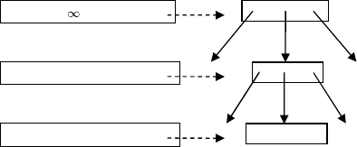
5.4 Index-to-index Navigation 319
A sorted set of search keys permits efficient navigation within the
B-tree. Most importantly, each page is needed only once, leaf pages
for a short duration and branch nodes for a longer duration. Once the
search has moved to a node’s neighbor with higher keys, the node can
be discarded in the buffer pool; there is no need to retain it using
a heuristic replacement strategy such as LRU. Thus, the buffer pool
needs to provide only one page per B-tree level plus appropriate buffer
frames for prefetch and read-ahead. Given that most B-trees have a
large fan-out and thus a very small height, it is reasonable to keep all
pages on the current root-to-leaf path pinned in the buffer pool. In addi-
tion, if the highest key read so far in each level of the B-tree is cached
(typically together with the data structures created when the B-tree is
“opened” for access by a query execution plan), it is not required that
each individual search starts with the root page. Instead, each search
can try B-tree pages in leaf-to-root order. Information about the most
recent update of each page, e.g., ARIES log sequence numbers [95],
can ensure that concurrent updates cannot interfere with the efficient
B-tree retrieval. Fence keys in B-tree nodes [44] can ensure that range
comparisons are accurate. Cheng et al. [25] describe a slightly more gen-
eral technique for unsorted sequences of search keys exploiting parent
pointers within disk pages rather than pinning in the buffer pool.
Figure 5.10 illustrates parts of the B-tree of Figure 2.4 and the
cache that enables efficient navigation within the B-tree during the
next search. The right half of Figure 5.10 shows data pages in the buffer
pool; the left half of Figure 5.10 shows part of the state associated with
the scan or the query operation. If the last search key was 17, the cache
contains pointers into the buffer pool for the three nodes shown plus the
7 89
23
15
17
23
19
High key , Page LSN …
High key 89, Page LSN …
High key 23, Page LSN …
Fig. 5.10 Cache state in pre-sorted index fetches.
320 Query Processing
high key and the Page LSN for each node. If the next search pertains
to key value 19, the cache is immediately useful and is best exploited
by starting the search at the leaf level. If the next search pertains to
key value 47, the current leaf must be abandoned but its immediate
parent continues to be useful. The high key of the parent node is 89 as
had been learned from the separator key in the root node. If the next
search key pertains to key value 99, both the leaf and its parent must
be abandoned and only the cached root node of this B-tree is useful.
The optimal starting level for each new search can be found with a
single comparison per B-tree level.
There are several difficulties if modifications of the B-tree structure
can lead to de-allocation of B-tree pages. For example, if the shown
leaf node is merged into a neighboring leaf due to a deletion and an
underflow, something must ensure that the search does not rely on an
invalid page in the buffer pool. This problem can be solved in various
ways, for example by verification of all Page LSNs along the root-to-leaf
path.
In order to enable these optimizations, the search keys may require
an explicit sort operation prior to the B-tree look-ups. In a sort of
search keys, expensive temporary files can be avoided in three ways. The
first way is a large memory allocation. The second one is to perform
merely run generation and invoking the searches with only partially
sorted search keys. This might be called an opportunistic sort, as it
opportunistically exploits the readily available memory and creates as
much ordering in its output as possible.
The third way employs a bitmap for compression and for sorting.
This method only works if there is a sufficiently dense bidirectional
mapping between search arguments and positions in a bitmap. More-
over, this mapping must be order-preserving such that scanning the
bitmap produces sorted search keys. Finally, this works for navigation
from a secondary index to the primary index of the same table, but it
does not work if any information obtained in earlier query operations
must be saved and propagated in the query execution plan.
Figure 5.11 continues Figure 5.9 using bitmaps. The illustration
employs hexadecimal coding for brevity, indicated by the prefix 0x for
each block of 4 digits or 16 bits. Given that bitmaps often contain many

5.4 Index-to-index Navigation 321
Compressed
Intermediate result
26-34, 42-43, 57, 98
Bitmap (hexadecimal) 0x0000, 0x0020, 0x2030, …
Compressed bitmap 3×0x00, 2×0x20, 1×0x30, …
Mixed representation 3×0x00, 0x2020, 0x30, 57, 98
Fig. 5.11 Bitmap compression for prefetch hints.
zeroes, run-length encoding of similar bytes is a standard technique, at
least for bytes containing all zeroes. Finally, the most compressed and
concise lossless representation interleaves run-length encoding, explicit
bitmaps, and lists of explicit values. Moreover, in order to avoid exter-
nal sorting, the representation may interleave compression techniques
without and with information loss.
The various compression methods can be combined. The goal is to
reduce the size such that the entire set of references can be retained
and sorted in memory, without expensive accesses to lower levels in
the storage hierarchy. If compression introduces any information loss
for some key range, all B-tree entries in that range must be scanned
during B-tree access, including re-evaluation of the appropriate query
predicates. In other words, repeated B-tree searches within the affected
key range have been turned into a range scan. Figure 5.9 shows an
example. If distribution skew is a concern, histograms (commonly used
for query optimization) can aid the choice of search keys most promis-
ing for compression. If information in addition to the references must
be carried along in the query execution plan, i.e., if the intention of
the index is to cover the given query, then only lossless compression
techniques are applicable.
Sorting the set of search keys improves query execution perfor-
mance [30, 96] but also the robustness of performance [52]. If cardinality
estimation during query optimization is very inaccurate, perhaps even
by several orders of magnitude, sorting the search keys into a single
sorted stream and optimizing the B-tree navigation ensure that index-
to-index navigation performs no worse than a table or index scan.
Figure 5.12 shows the performance of the same two traditional plans
shown in Figure 5.5 as well as the cost of a robust plan. For small
query results, sorting the references obtained from the secondary index
hardly affects the execution cost. For large query results, sorting the

322 Query Processing
Qualifying rows
0%
100%
Execution cost
0
Index scan plus record fetch
Table scan
Robust scan
Fig. 5.12 Robust transition between index scan and table scan.
references ensures that the cost never exceeds that of a table scan by too
much. The difference is for obtaining and sorting the references from a
secondary index. If the record size in the secondary index is a fraction
of that in the primary index, the scan cost in the secondary index is
the same fraction of the scan cost of the primary index. Appropriate
compression ensures that the sort operation can rely on internal sort
algorithms and does not contribute I/O operations to the overall query
execution cost.
Thus, Figure 5.12 illustrates a prototypical example of robust index-
to-index navigation. Similar techniques apply also to complex queries
that join multiple tables, not just to navigation among multiple indexes
of the same table.
If a secondary index is used to provide an “interesting order-
ing” [115], e.g., for a subsequent merge join, and if the secondary index
is not a covering index for the table and the query, either the merge
join must happen prior to fetching full records, or the fetch opera-
tion must not sort the references and thus forgo efficient retrieval, or
the fetched records must be sorted back into the order in which there
were obtained from the secondary index. The latter method essentially
requires another sort operation.
One idea for speeding up this second sort operation is to tag the
records with a sequence number prior to the first sort such that the
second sort can be efficient and independent of the type, collation
sequence, etc. in the original secondary index. On the other hand, this
sort operation must manage larger records than the sort operation prior
to the join and it cannot benefit from compression, particularly from

5.4 Index-to-index Navigation 323
Nested iteration
Sort (for fast access) Primary index
Secondary index
Sort (for interesting order)
Fig. 5.13 Sorting for a robust join and sorting “back.”
compression with information loss. Thus, this sort operation may be
an external sort even when the initial sort operation is not.
Figure 5.13 shows a fragment of a query execution plan in which
this technique could be beneficial. A secondary index provides records
in a sort order “interesting” for a subsequent operation such as a merge
join (not shown in Figure 5.13) yet, for robust retrieval from a primary
index, an alternative sort order is required. With appropriate tech-
niques, the performance of the final sort may be improved by exploiting
the sort order in the secondary index.
In order to support index-to-index navigation among multiple
tables, a promising heuristic is to include all key columns in all
secondary indexes, both primary key columns and foreign key columns.
The difference between the query execution plans in Figures 5.6 and 5.7
illustrate the beneficial effect. The technique can be extended by includ-
ing columns of other tables based of functional dependencies and for-
eign key constraints. For example, an index on a date column of a table
of order details might include a customer identifier; the order details
table typically does not include this column but there is an appropriate
functional dependency in the orders table.
•
If an index needs to be probed with many search keys, sorting
the keys avoids duplicate searches and may improve buffer
pool effectiveness and thus I/O costs.
•
An index search may resume where the preceding search left
off, resulting in both upward and downward navigation in a
B-tree index.
324 Query Processing
•
These optimizations enable robust query execution plans
with a graceful transition from fetching only a few items
based on a secondary index to scanning a primary index
completely, thus reducing surprising performance due to
erroneous cardinality estimation during compile-time query
optimization.
•
The break-even point between optimized scans (e.g., in
compressed column stores) and optimized index retrieval may
shift with the transition from traditional high-latency disk
storage to semiconductor storage such as flash.
5.5 Exploiting Key Prefixes
Most of the discussion so far has assumed that a search in a B-tree starts
with a complete key, i.e., specific values for all the fields in the B-tree
key. The output of the search was the information associated with a key,
e.g., a pointer to a record in the primary index or the heap file. Since
all B-trees are unique, if necessary by adding something to the user-
defined key, such B-tree searches produce at most one matching record.
While some indexes support only searching with precise values of the
entire index key, notably hash indexes, B-trees are far more general.
Most importantly, B-trees support range queries for records with
key values between given lower and upper bounds. This applies not
only entire fields in a key but also prefixes within a column value, in
particular a string value. For example, if a B-tree key field contains
names such as “Smith, John,” a query for all persons with the last
name “Smith” is effectively a range query, as would be queries for
names starting with “Sm” or for “Smith, J.”
It is commonly believed that a B-tree is useful only if the search key
in the query specifies a strict prefix of the B-tree key, but this is not
the case. For example, in a B-tree organized by zip code (postal code)
and (family) name, finding all people with a specific name requires
enumeration of all distinct zip code values in the B-tree and searching
for the specified name once for each zip code. The enumeration of zip
codes can precede the search by name or the two can be interleaved [82].
Moreover, after the search within one zip code is complete, the next step

5.5 Exploiting Key Prefixes 325
1,a 1,z 2,a 2,z 3,a 3,z 5,a 5,z
… … … …
Fig. 5.14 Two-column B-tree index.
can search for the next zip code using the B-tree index or it can simply
add one to the prior zip code and attempt to find the combination
of the incremented zip code and the desired name. If the attempt fails
because the incremented zip code does not exist, the root-to-leaf search
in the B-tree leads to a record with the next actual value in the zip
code column.
Figure 5.14 shows a B-tree index with a two-column key. For a query
that specifies only the letter column but not the number column, e.g.,
“where letter = ‘q’ ,” an enumeration of the number values is required.
The first root-to-leaf traversal of the B-tree finds the number 1 or actu-
ally the combined key “1,a”; the first search probes for a combined key
of “1,q.” The next root-to-leaf traversal might be employed to find
the number 2 in the combined key “2,a” by looking for a B-tree entry
with a number larger than 1. In the improved scheme, the number 2
is not found in a search but calculated from the prior value 1, and the
next root-to-leaf search focuses immediately on the combined key “2,q.”
This works well for number values 2 and 3. The root-to-leaf traversal
in search of the combined key “4,q” fails to find an appropriate record
but it finds a record with number value 5. Thus, the next search might
search directly for the combined key “5,q.”
This technique seems most promising if the number of distinct values
is fairly small (zip codes in the example above or number values in
Figure 5.14). This is because each distinct leading B-tree key value
requires a single random I/O to fetch a B-tree leaf. The number of dis-
tinct values is not the true criterion, however. The alternative query exe-
cution plan typically is to scan the entire index with large sequential I/O
operations. The probing plan is faster than the scanning plan if the data
volume for each distinct leading B-tree key value is so large that a scan
takes longer than a single probe. Note that this efficiency comparison
must include not only I/O but also the effort for predicate evaluation.
326 Query Processing
In addition to unspecified leading B-tree keys as in the example
of a specific name in any zip code area, a leading column may also be
restricted by a range predicate rather than a specific value. For example,
the zip code might be restricted to those starting “537” without regard
for the last two digits. Moreover, the technique also applies to more than
two columns: the first column may be restricted to a specific value, the
second column unspecified, the third column restricted to a range, the
fourth column unspecified, and the fifth column restricted to a specific
value again. The analysis of such predicates may be complex but B-trees
seem to support such predicates better than other index structures.
Perhaps the most complex aspect is the cost analysis required for a cost-
based compile-time decision between a full index scan, range scan, and
selective probes. A dynamic run-time strategy might be most efficient
and robust against cardinality estimation errors, cost estimation errors,
data skew, etc.
In a B-tree index with a key consisting of multiple fields, the
individual fields may be thought of as forming a hierarchy or as repre-
senting dimensions in a multi-dimensional space. Thus, a multi-column
B-tree might be considered as a multi-dimensional access method
(MDAM) [82]. If a leading dimension is under-specified in the query
predicate, its possible values must be enumerated. This strategy works
well if the dimensions are measured in integer coordinates and the num-
ber of distinct values in the leading dimensions. By transforming the
query predicate into appropriate range queries in the sort order of the
B-tree, even complex disjunctions and conjunctions can be processed
quite efficiently [82].
The techniques illustrated in Figure 5.10 enable dynamic and auto-
matic transitions between probing a B-tree with root-to-leaf traversals
and scanning a B-tree in index-order. After a few recent requests could
be satisfied by the current leaf or its immediate neighbor, asynchronous
read-ahead of subsequent leaf nodes based on parent and grandparent
nodes seems promising. If reuse of leaf nodes is rare but parent nodes
and their immediate neighbors are useful in successive search requests,
leaf nodes might be evicted quickly from the buffer pool but asyn-
chronous read-ahead might be applied to parent nodes.
5.6 Ordered Retrieval 327
•
Compound (i.e., multi-column) B-tree indexes support equal-
ity predicates on any prefix of their columns.
•
With clever analysis of predicates, B-trees also support mix-
tures of range and equality predicates on subsets of their
columns, even including cases with no restriction on the lead-
ing column.
5.6 Ordered Retrieval
Just like B-trees can provide more kinds of searches than is commonly
realized, they can also support a larger variety of sort orders in the
output of a scan. Coming back to the earlier idea of a B-tree as a cached
state of a sort operation, the most obvious sort order has the B-tree
keys as ordering keys. Ascending and descending orders are supported
equally well in most implementations. Any sort order on a prefix of the
B-tree key is also supported.
If the desired sort key starts with a prefix of the B-tree but also
includes columns present in the B-tree but not in a useful way in the
B-tree key, then it can be beneficial to execute a sort operation for each
distinct value in the useful prefix columns of the B-tree. For example,
if a table with columns A,B,C,...,X,Y,Z is stored in a primary index
on columns A, B,C, and if a query requires output sorted on A, B,P,Q,
then it is possible to exploit the sort order on A,B and sort records on
P,Q for each distinct pair of values of A, B. Ideally, this sequence of
smaller sort operations can be faster than a single large sort operation,
for example because all or most of these small sort operations can be
executed in memory whereas the single large sort would require run
files on disk. In that case, this execution strategy requires (most of)
the run generation effort of the large sort but not its merge effort.
Figure 5.15 illustrates these individual, small sort operations using
the dashed brackets. The sizes of individual segments may vary widely
such that some but not all segment may fit in the available memory
allocation.
If, on the other hand, the desired sort order omits a prefix but
otherwise matches the B-tree key, the distinct values of the omitted

328 Query Processing
A=1, B=1 A=1, B=2 A=1, B=3 A=2, B=1
Fig. 5.15 Sort once for each distinct pair A, B.
A=2A=1 A=3
Fig. 5.16 Sort by merging runs identified by distinct values of A.
prefix columns can be thought of identifiers of runs in an external merge
sort, and the desired sort order can be produced by merging those runs.
Using the same example table and primary index, if a query requires
output sorted on B, C, then the B-tree can be thought as many runs
sorted on B, C and the distinct values of A identify those runs. This
execution strategy requires the merge effort of the large sort but not
its run generation effort.
Figure 5.16 illustrates the merge step that scans the primary index
on A, B,C once for each individual value of A and then merges runs
identified by distinct values of A. If the count of distinct values of A
is smaller than the maximal merge fan-in (dictated by the memory
allocation and the unit of I/O), a single merge step suffices. Thus, all
records are read once and, after passing through the merge logic, ready
for the next step with run generation, run files on disk, etc.
These two techniques can be combined. For example, if a query
requests output sorted on A,C, then the distinct values of A enable
multiple small sort operations, each of which merges runs sorted on C
and identified by distinct values of B. Note that the number of dis-
tinct values of B might vary for different values of A. Thus, the small
sort operations might require different merge strategies. Thus, merge
planning and optimization require more effort than in a standard sort
operation. More complex combinations of these two techniques are also
possible.

5.7 Multiple Indexes for a Single Table 329
Sorted output is required not only upon explicit request in the
query text but also for many query execution algorithms for joins, set
operations such as intersection, grouped aggregation, and more. “Top”
queries for the most important, urgent, or relevant data items benefit
from the sort and merge strategies described above because the first
output is produced faster than by a large sort operation that consumes
its entire input before producing its first output. Similar considera-
tions apply to queries with “exists” clauses if the inner query employs
an order-based algorithm such as a merge join.
•
In addition to any prefix, a B-tree can produce sorted output
on many other variations of its column list using merging or
segmented execution.
•
These techniques assist many order-based query evaluation
algorithms and apply to any source of pre-sorted data, not
only B-trees.
5.7 Multiple Indexes for a Single Table
Most query execution strategies discussed above exploit at most one
index per table. In addition, there are many strategies that exploit
multiple indexes, for example for multiple predicates.
For a conjunction of two or more predicate clauses, each matching
a different index, the standard strategy obtains a list of references from
each index and then intersects these lists. For a disjunction, the union
of lists is required. Negated clauses call for difference operations.
Figure 5.17 shows a typical query execution plan for a query with
a conjunction predicate executed by intersecting lists of references
Secondary index
Name
Bitmap intersection
Secondary index
Zip code
Nested iteration
Primary index
Fig. 5.17 Index intersection for a conjunctive predicate.
330 Query Processing
obtained from multiple indexes for the same table. The result lists from
each secondary index are transformed into a bitmap if the indexes are
not bitmap indexes, their intersection is computed, and complete rows
are fetched for the table using an index nested loops join.
Set operations such as intersection can be processed with standard
join algorithms such as hash join or with bitmaps. If bitmaps are
not compressed, hardware instructions such as “binary and” can be
exploited. If bitmaps are compressed with run-length encoding or one
of its variants, appropriate merge logic enables set operations with-
out decompression. Alternatively, disjunctions and negations can be
processed using a single bitmap, with multiple index scans setting or
clearing bits.
Another type of multi-index strategy exploits multiple indexes on
the same table to achieve the performance benefits of covering indexes
even when a single covering does not exist. Scanning and joining two
or more secondary indexes with few columns and thus short records
can be faster than scanning a primary index or heap with long records,
depending on the efficiency of the join operation and the availability
of sufficient memory [52]. A query execution plan with two indexes
covering a query is shown in Figure 5.8 in Section 5.3. It differs from
the query execution plan in Figure 5.7 by avoiding the nested iteration
to look up rows and by join rather than an intersection operation.
In some join queries, the best plan employs multiple indexes for
each of the tables. For example, secondary indexes can be employed
for semi-join reduction [14]. The goal is to reduce the list of rows
to be fetched not only by single-table selection predicates but also
by multi-table join predicates. Thus, secondary indexes from differ-
ent tables are joined first based on the join predicate in the query. This
assumes, of course, that the columns in these secondary indexes cover
the join predicate. The cost of then fetching rows from the two tables’
primary indexes is incurred only for rows that truly satisfy the join
predicate.
Figure 5.18 shows a query execution plan joining two tables using
semi-join reduction. The essential aspect of the query execution plan
in Figure 5.18 is that the join predicate is evaluated before rows are
fetched from the tables. The order in which tables (or their indexes) are

5.7 Multiple Indexes for a Single Table 331
Secondary index
Course.Course-number
Merge join
Secondary index
Enrollment.Course-number
Index nested
loops join
Primary index
Enrollment
Index nested loops join
Primary index
Course
Fig. 5.18 Two-table semi-join reduction.
joined is independent of the order in which tables are accessed to fetch
missing column values. In this specific example, referential integrity
constraints (courses only exist with enrolled students, enrollments must
refer to existing courses) may be defined in the database. If so, semi-
join reduction may be ineffective unless there are additional predicates
not shown in the diagram, e.g., on titles of courses or on grades in the
enrollment table, that invalidate the referential integrity constraints.
The technique applies to complex joins with multiple tables and
has proven particularly valuable for complex joins with one particularly
large table, also known as the central “fact table” in a “star schema”
in relational data warehousing. In the typical “star queries” over such
databases, the predicates often apply to the “dimension tables” sur-
rounding the fact table, but the query execution cost is dominated
by the accesses to the large fact table. In one of the standard query
optimization techniques for such “star joins,” the dimension tables are
joined first with secondary indexes of the fact table, the resulting lists
of row identifiers in the fact table are combined into a single list of
rows that satisfy all predicates in the query, and only the minimal
set of rows from the fact table is fetched as a last step in the query
execution plan.
Figure 5.19 shows a query execution plan for a star join using both
index intersection and semi-join reduction. The original query includes
predicates on the two dimensions “customer” (e.g., “city = Big Sky,
Montana”) and “part” (e.g., “part name = “boat anchor”). Note that
star queries often involve correlations far beyond the semantic capa-
bility of database statistics and metadata. For example, few customers

332 Query Processing
Dimension “customer”
with predicate
Hash right semi join
Secondary index on
Sales-facts.customer-id
Dimension “part”
with predicate
Hash right semi join
Secondary index
On sales-facts.part-no
Hash intersection
Nested iteration
Table Sales-facts
Fig. 5.19 Star join using intersection and semi-join reduction.
will purchase boat anchors high in the mountains. In the query execu-
tion plan of Figure 5.19, each of the two initial join operations performs
a semi-join between a dimension table and the appropriate secondary
index of the fact table. The result is a set of references in the fact
table. The intersection operation produces the references in the fact
table for rows satisfying the predicates on both dimensions. The final
right semi-join produces these fact rows. If it is desirable that columns
from a dimension table are preserved, the appropriate initial semi-join
and the final semi-join must be inner joins instead.
A related issue that is often neither understood nor considered is
concurrency control among multiple indexes of the same table, in par-
ticular if a weak transaction isolation level is chosen. If predicate eval-
uation is performed in multiple indexes yet concurrency control fails to
ensure that matching index entries in multiple indexes are consistent,
a query result may include rows that fail to satisfy the overall query
predicate and it may fail to include rows that do satisfy the predicate.
This issue also applies to predicates across multiple tables, but per-
haps users relying on weak transaction isolation levels are more likely
to expect weak consistency between tables than within an individual
row of a single table. This issue also exists between materialized views
and their underlying tables, even if incremental view maintenance is
part of each update transaction.
•
Index intersection can speed up conjunctive predicates and
is commonly used. Index union can support disjunctions and

5.8 Multiple Tables in a Single Index 333
index difference can support “and not” predicates. Bitmaps
can enable efficient implementations of these operations.
•
Multiple indexes together may cover a query in a special case
of index-only retrieval.
•
In data warehouses with star or snowflake schemas, sophisti-
cated index usage may be required for optimal performance.
5.8 Multiple Tables in a Single Index
Since join operations are traditionally among the most expensive
database query operations, and since most joins are specified with
the same equality predicates on foreign keys and primary keys, two
techniques suggest themselves that combine multiple tables in a single
index.
First, a join index maps values of join columns to references in two
(or more) tables [66, 123]. These references may be represented by lists
or by bitmaps [105]. Scanning a join index produces a result similar to
that of joining two secondary indexes on the respective join columns.
Figure 5.20 illustrates the combined image for 3 tables as proposed
by H¨arder, including a key value, occurrence counters for each of the
tables, and the appropriate number of record identifiers in the tables.
It is not required that every key value occurs in each table; counters
might be zero.
A “star index” [33] is very similar to combined images and to join
indexes. The main difference is that the star index contains record
references in the dimension tables rather than key values. In other
words, a star index maps record references in the appropriate dimension
tables to record references in a fact table. If the star index is a B-tree,
the order of the dimension tables in records of the star index matters,
with the best clustering achieved for the dimension table mentioned
Key 1 3 2 RID RID RID RID RID RID
Counters
Table 1 Table 2
Table 3
Fig. 5.20 Combined image proposed by H¨arder.

334 Query Processing
first. If the record references in all dimension tables are column values,
e.g., the primary key or the clustering key of the dimension table, then
the star index is practically the same as a multi-column B-tree index
on the corresponding foreign key values in the fact table.
Second, merged indexes are discussed in Section 7.3.
•
Join indexes and star indexes combine multiple secondary
indexes into a single B-tree in order to speed up large joins.
5.9 Nested Queries and Nested Iteration
1
Database and disk sizes continue to grow fast, whereas disk access
performance and disk bandwidth improve much more slowly. If for no
other reason than that, research into database query processing must
refocus on algorithms that grow linearly not with the database size but
with the query result size. These algorithms and query execution plans
rely very heavily on index navigation, i.e., they start with a constant
given in the query predicate, find some records in an index, extract
further column values from those records, find more records in another
index, and so on. The cost of this type of query plan grows linearly
with the number of records involved, which might very well mean that
the cost is effectively independent of the database size. Actually, the
cost of index look-ups in traditional B-tree indexes grows logarithmi-
cally with the database size, meaning the cost doubles as a table grows
from 1,000 to 1,000,000 records, and doubles again from 1,000,000 to
1,000,000,000,000 records. The cost barely changes from 1,000,000 to
2,000,000 records, whereas the cost of sort or hash operations doubles.
Moreover, it is well known that scanning “cleans” the I/O buffer of
all useful pages, unless the replacement policy is programmed to rec-
ognize scans [26, 91, 120]. It is not unlikely, however, that CPU caches
and their replacement policies recognize scans; thus, large scans will
repeatedly clear out all CPU caches, even level-2 and level-3 caches of
multiple megabytes. Based on these behaviors, on the growth rates of
disk sizes and disk bandwidths, and on the recent addition of materi-
alized and indexed views to mainstream relational database systems,
1
Some of this section is derived from [42].

5.9 Nested Queries and Nested Iteration 335
we should expect a strong resurgence of index-based query execution
and thus research interest in execution plans relying heavily on nested
iteration. The advent of flash storage with access latencies 100 times
faster than traditional disk drives will speed this trend.
The key to interactive response times, both in online transaction
processing (OLTP) and in online analytical processing (OLAP), is to
ensure that query results are fetched, not searched and computed. For
example, OLAP products perform well if they can cache the results of
prior and likely future queries. In relational database systems, fetching
query results directly means index searches. If a result requires records
from multiple indexes, index nested loops join or, more generally, nested
iteration are the algorithms of choice [63].
Figure 5.21 shows a query evaluation plan for a simple join of three
tables, with the “outer” input of nested iterations shown as the left
input. The nested iterations are simple Cartesian products here, as the
join predicates have been pushed down into the inner query plans. If the
filter operations are actually index searches and if table T0 is small
relative to T1 and T2, this plan can be much more efficient than any
plan using merge join or hash join. An alternative plan uses multiple
branches of nested iteration rather than multiple levels as the plan in
Figure 5.21. Of course, complex plans might combine multiple levels
and multiple branches at any level.
Nested loops join is the simplest form of nested iteration. There
is no limit to the complexity of the inner query. It might require
searching a secondary index and subsequently fetching from the main
Nested iteration binds T0.a and T0.c
Filter T2.b =
T1.b and T2.c < T0
Table T0
Table T1 Table T2
Filter T1.a = T0.a
Nested iteration binds T1.b
Fig. 5.21 Query plan with nested iteration.
336 Query Processing
table; intersecting two or more secondary indexes using bitmap, sort, or
hash operations; joining multiple tables each with its own access paths;
multiple levels of nested iteration with multiple sub-branches at each
level; etc. For all but the most trivial cases, there are complex issues
that need to be addressed in a commercial product and in a complete
research prototype. These issues exist at the levels of both policies and
mechanisms, with avoiding I/O or exploiting asynchronous I/O as well
as with managing resources such as memory and threads.
In addition to the techniques described earlier for asynchronous
prefetch, sorting references before fetching rows, etc., B-tree indexes
can also play an important role for caching the results of inner queries.
Conceptually, one might want to employ two indexes, one for previously
encountered outer binding values (parameters of the inner query), and
one for results of inner query. The latter may contain many records
for each of many outer bindings, and thus may grow quite large. The
former might include also the result size as well as frequency or recency
of usage. Information about empty results may prevent repeated futile
searches and information about actual result sizes and usage may guide
replacement decisions, e.g., in order to retain the most valuable inner
results in a CPU cache or a buffer pool. This index may even be used
to guide which outer binding to process next, e.g., producing results
immediately for outer bindings with empty inner results. Note that
those two indexes might be retained in a single merged B-tree such
that any overhead due to separating the cache into two indexes is
minimized.
•
In query processing based on scans, query execution times
grow with the table or database size. In query processing
based on index-to-index navigation, query execution times
grow with the size of intermediate results and are hardly
affected by database or table size.
•
Nested loops join is the simplest form of nested iteration.
In general, the inner query execution plan can be complex,
including multiple levels of nested iteration.
•
Sorting the outer bindings is as helpful for general nested
iteration as for index nested loops join.
5.10 Up date Plans 337
•
Nested iteration can be very efficient if tables accessed by
the inner query are very small or indexed.
5.10 Update Plans
In order to enable these various index-based query execution strate-
gies, indexes must exist and must be up-to-date. Thus, the issue of
efficient index creation and index maintenance is a necessary comple-
ment to query processing. In the following discussion, updates include
modifications of existing records, insertions, and deletions.
Various strategies for efficient index maintenance have been
designed. These include sorting changes prior to modifying records
and pages in B-trees, splitting each modification of an existing record
into a deletion and an insertion, and a choice between row-by-row and
index-by-index updates. The row-by-row technique is the traditional
algorithm. When multiple rows change in a table with multiple indexes,
this strategy computes the delta rows (that include old and new values)
and then applies them one by one. For each delta row, all indexes are
updated before the next delta row is processed.
The index-by-index maintenance strategy applies all changes to the
primary index first. The delta rows may be sorted on the same columns
as the primary index. The desired effect is similar to sorting a set of
search keys during index-to-index navigation. Sorting the delta rows
separately for each index is possible only in index-by-index mainte-
nance, of course.
This strategy is particularly beneficial if there are more changes
than pages in each index. Sorting the changes for each index ensures
that each index page needs to be read and written at most once.
Prefetch of individual pages or large read-ahead can be used just as
in read-only queries; in addition, updates benefit from write-behind.
If read-ahead and write-behind transfer large sequences of individual
pages as a single operation, this strategy is beneficial if the number of
changes exceeds the number of such transfers during an index scan.
Figure 5.22 shows parts of a query execution plan, specifically those
parts relevant to secondary index maintenance in an update statement.
Not shown below the spool operation is the query plan that computes

338 Query Processing
Sort
Collapse
Update index
Split
Spool
Sort
Update index
Split Sort
Update index
Fig. 5.22 Optimized index maintenance plan.
the delta to be applied to a table and its indexes. In the left branch,
no columns in the index’s search key are modified. Thus, it is sufficient
to optimize the order in which changes are applied to existing index
entries. In the center branch, one or more columns in the search key
are modified. Thus, index entries may move within the index or, alter-
natively, updates are split into deletion and insertion actions. In the
right branch, search key columns in a unique index are updated. Thus,
there can be at most one deletion and one insertion per search key in
the index, and matching deletion and insertion items can be collapsed
into a single update item, which might save root-to-leaf B-tree traver-
sals as well as log volume. In spite of the differences among the indexes
and how they are affected by the update statement, their maintenance
benefits from sorting, ideally data-driven sort operations.
The implementation of index-by-index maintenance may use a plan
with multiple operations, which is very similar to a query execution
plan. The maintenance operations for the secondary indexes may form
a long chain with change rows passing from one to the next, or the
change rows may be a shared intermediate result typically implemented
with intermediate storage. Both update plans modify one secondary
index after another. The long chain might seem easier to schedule but
it requires that the earlier sort operations carry along all fields needed
in subsequent index updates. In the update plan shown in Figure 5.22,
this is avoided, at the expense of writing and reading the change set
with all columns in the spool operation.
5.10 Up date Plans 339
For additional efficiency, the spool operation can be avoided or,
more accurately, integrated into the sort operations. Specifically, a
single sort operation at the bottom of this plan fragment could receive
input data, save those records in its workspace, and then generate
runs for all three branches. For each branch, the sort operation must
create an array with one or two surrogates per record in the workspace.
Two surrogates are required for branches that show a split opera-
tion in Figure 5.22. This multi-function sort operation writes precisely
the same records to runs on disk as the multiple sort operations in
Figure 5.22. The savings are writing and reading the change set with
all its columns in the spool operation and copying data into multi-
ple sort operations’ workspaces; the disadvantage is that all columns
are present in the workspace during run generation, resulting in more,
smaller runs and possibly additional merge steps.
In this update plan, the sort operation competes for resources, most
notably memory, with the operations computing the change set and
preparing it, probably sorting it, for updating the primary index. Thus,
intermediate runs in the sort operations as shown in Figure 5.22 may be
more efficient than an integrated sort operation. Another variant of the
algorithm seems desirable if the in-memory workspace is sufficient to
sort the entire change set without the need for temporary runs. Thus,
it is no surprise that database systems differ in the variety of optimiza-
tions implemented for large updates of indexed tables and materialized
views.
Another technique enabled by index-to-index maintenance is per-
index protection against the Halloween problem [90]. In general, search-
ing and updating an index in the same plan phase may lead to incorrect
updates or even infinite loops. Since a sort operation creates separate
plan phases, it is possible to exploit one or more secondary indexes to
compute the change rows and to apply those changes immediately to
the primary index.
Finally, the basic ideas of index-by-index maintenance and update
plans also apply to foreign key constraints, materialized view and their
indexes, and even triggers. Specifically, foreign key constraints may be
verified using branches in an update plan quite similar to maintenance
of an individual secondary index, and cascading of information for
340 Query Processing
foreign key constraints and materialized views can be achieved in addi-
tional branches. Plan creation in complex databases is a challenge in
its own right; for the purposes of this survey focused on B-tree indexes,
it is sufficient to realize that various techniques for very efficient index
maintenance are already implemented in some database management
systems.
•
Index maintenance can be optimized as much as index-
to-index navigation during read-only query execution. The
principal choice is index maintenance row-by-row or index-
by-index. Similar choices pertain to checking integrity
constraints.
•
Sorting updates for each index can speed up index main-
tenance. Sorting can also provide protection from the
Halloween problem due to its separation of input phase and
output phase.
5.11 Partitioned Tables and Indexes
Partitioning divides a single table into multiple data structures. Among
the basic forms of partitioning, horizontal partitioning defines subsets of
rows or records whereas vertical partitioning defines subsets of columns
or fields. In each form of partitioning, these subsets usually are disjoint.
In other words, partitioning does not introduce redundancy.
In a partitioned table or index, each partition is kept in its own data
structure, often a B-tree. Each partition and its B-tree are registered
in the database catalogs. Since creation and removal of a partition
must be recorded in the database catalogs, appropriate permissions
and concurrency control in the catalogs are required. In contrast, a
partitioned B-tree [43] keeps multiple horizontal partitions in a single
B-tree. B-tree entries belong to the partition identified by the artificial
leading key field in each record. Partitions are created and removed
simply by insertion or deletion of appropriate records and their key
values.
Horizontal partitioning can be used for manageability and as a
coarse form of indexing. Manageability can be improved by partitioning
on a time attribute such that load and purge operations, also known
5.11 Partitioned Tables and Indexes 341
as roll-in and roll-out, always modify entire partitions. As a form of
indexing, partitioning directs retrievals to a subset of a table. If most
queries need to scan data equivalent to a partition, partitioning can be
a substitute for indexing. In some cases, multi-dimensional partitioning
can be more effective than single-dimensional indexing.
Vertical partitioning, also known as columnar storage, enables effi-
cient scans when appropriate indexes are not available to guide the
search. Some claim that a data structure with only one column and
data type permits more effective compression and therefore faster scans;
others believe that equally effective compression is possible in both row
storage and column storage [108]. In addition to compression, scan effi-
ciency benefits from transferring only those columns truly needed in
query execution plan. On the other hand, result rows must be assem-
bled from column scans and exploiting shared or coordinated scans
might be more complex for columnar storage.
Query execution plans often must treat partitioning columns and
partition identifiers quite similarly to search keys in primary indexes.
When sorting search keys in index-to-index navigation, the partition
identifier should be a minor sort key; if the partition identifier is the
major sort key, partitions will be searched one after the other rather
than in parallel. Depending on key distributions, a more sophisticated
mapping from reference to sort key might be required in some cases.
Many such considerations and techniques also apply to updates.
When updating the partitioning key, index entries might need to move
from one partition to another; this requires splitting the update into
deletion and insertion. In other words, what is a performance optimiza-
tion in non-partitioned indexes might be a requirement in partitioned
indexes.
•
Tables and indexes can be partitioned horizontally (by rows)
or vertically (by column).
•
A secondary index is local if it is partitioned horizontally
in the same way as the primary data structure of the table.
References from the secondary index to the primary data
structure do not require partition identifiers as in a global
index.
342 Query Processing
•
Most strategies for index-to-index navigation during query
execution and for index maintenance require some adapta-
tion in case of partitioned tables and indexes.
5.12 Summary
In summary, there is a large variety of techniques to make optimal use
of B-tree indexes in query execution plans and update execution plans.
Na¨ıve or incomplete implementation of query optimization or query
execution reduces the value of B-tree indexes in databases. It seems
that all actual implementations fall short in one dimension or another.
Therefore, creation, maintenance, scans, search, and joins of indexes
continue to be a field of innovation and of competition. With databases
stored on flash devices instead of traditional disk drives, hundred-fold
faster access times will increase the focus on index data structures and
algorithms.

6
B-tree Utilities
In addition to the wide variety of efficient transactional techniques and
query processing methods exploiting B-tree indexes in databases, per-
haps it is really the large set of existing utilities that separates B-trees
from alternative indexing techniques. For example, a B-tree index struc-
ture in a database or on some backup media can be verified with a single
scan over the data pages, in any order, and with limited amounts of
temporary information retained in memory or on disk. Even efficient
index creation for large data sets often takes years to develop for a new
index structure. For example, more and more efficient strategies for
construction and bulk loading of R-tree indexes have been forthcom-
ing over a long time [23, 62] compared to simply sorting for efficient
construction of a B-tree index, which also applies to B-tree indexes
adapted to multiple dimensions [6, 109]. Comparable techniques for
alternative index structures are usually not part of initial proposals for
new indexing techniques.
Index utilities are often set operations, whether index creation by
preparing a set of future index entries or structural verification by
processing a set of index facts after extracting them from an index
such as a B-tree. Thus, many traditional query processing techniques
343
344 B-tree Utilities
can be employed in index utilities including query optimization (e.g.,
the choice among joining two secondary indexes of the same table
or scanning the table’s primary index), partitioning and parallelism,
workload management for admission control and scheduling, and
resource management for memory and temporary disk space or disk
bandwidth. Similarly, many transactional techniques can be employed
in index utilities that have already been discussed above. Thus, the
following discussion does not address implementation issues related
to space management, partitioning, non-logged operation, online
operation with concurrent updates, etc.; instead, the primary focus of
the following discussion is on aspects not yet covered but relevant for
database utilities for indexes in general and for B-trees in particular.
•
Utilities are crucial for efficient operation of a database and
its applications. More techniques and implementations exist
for B-trees than for any other index format.
•
Utilities often affect entire databases, tables, or indexes.
They often run a long time. Some systems employ techniques
and code from query optimization and query execution.
6.1 Index Creation
While some products initially relied on repeated insertions for index
creation, the performance of index creation is much improved by first
sorting the future index entries. Therefore, techniques for efficient index
creation can be divided into techniques for fast sorting, techniques for
B-tree construction from a sorted stream, techniques enabling parallel
index construction, and transactional techniques for index creation.
During B-tree construction from a sorted stream, the entire “right
edge” of the future B-tree may be kept and even pinned in the buffer
pool at all times in order to avoid effort on redundant search in the
buffer pool. Similarly, during online index creation, “large” locks [48]
may be retained as much as possible and released only in response
to a conflicting lock request. Alternatively, transactional locks may be
avoided entirely as index creation does not modify the logical database
contents, only their representation.

6.1 Index Creation 345
A new index is usually created with some free space for future inser-
tions and updates. Free space within each leaf node enables insertions
without leaf splits, free space within branch nodes enables splits in
the next lower B-tree level without splits cascading up the tree, and
free pages within allocation units (such as extents or disk cylinders)
enable splits without expensive seek operations during the split and,
much more importantly, during all subsequent range queries and index-
order scans. Not all systems give explicit control over these forms of
free space because it is difficult to predict which parameter values will
turn out to be optimal during future index usage. Moreover, the control
parameters might not be followed precisely. For example, if the desired
free space in each leaf is 10%, prefix B-trees [10] might choose the key
ranges of neighboring leaves such that the separator key is short and
the left node contains anywhere from 0% to 20% free space.
Figure 6.1 shows fixed-size pages with variable-size records imme-
diately after index creation. All pages are fairly but not necessarily
entirely full. After some number of pages (here 3), an empty page
remains readily available for future page splits.
In an index with non-unique key values, the sort order should
include sufficient reference information to render entries unique, as
discussed earlier. This will aid in concurrency control, in logging and
recovery, and in eventual deletion of entries. For example, when a log-
ical row is deleted in a table, all records pertaining to that row in all
indexes must be deleted. In a non-unique secondary index, this sort
order enables finding the correct entry to delete efficiently.
If a secondary index is “very non-unique,” i.e., there is a large set of
references for each unique key value, various compression methods can
reduce the size of the index as well as the time to write the initial index
to disk, to scan the index during query processing, or to copy the index
during a replication or backup operation. The most traditional repre-
sentation associates a counter and a list of references to each unique
Fig. 6.1 Free space immediately after index creation.

346 B-tree Utilities
… 6 4 4 4 2 1
… 10 7 5 3 3 2
… 4 4 4 3
… 3 3 3 2 2 1
Fig. 6.2 Avoiding comparisons without duplicate elimination.
key value [66]. In many cases, the numeric differences between neigh-
boring references can be represented more compactly than complete
reference values. The proper sort enables efficient construction of such
lists of differences; in fact, construction of such lists can be modeled as
an aggregation function and can thus reduce the data volume written
to temporary storage in an external merge sort. Bitmaps can also be
employed. Grouping future index entries based on equal key values as
early as possible not only enables compression and thus less I/O dur-
ing sorting but also fewer comparisons during the merge steps, because
only a single representative key value needs to participate in the merge
logic after entries have been grouped.
Figure 6.2 (from [46]) illustrates this point for a three-way merge.
Underlined keys are representatives of a group in the merge inputs and
in the merge output. Values 1, 2, and 3 are struck out in the merge
inputs because they have already gone through the merge logic. In the
inputs, both copies of value 2 are marked as representatives of a group
within their runs. In the output, only the first copy is marked whereas
the second one is not, to be exploited in the next merge level. For
value 3, one copy in the input is already not marked and thus did not
participate in merge logic of the present merge step. In the next merge
level, two copies of the value 3 will not participate in the merge logic.
For value 4, the savings promises to be even greater: only two of six
copies will participate in the merge logic of the present step, and only
one in six in the next merge level.
Another possible issue during creation of large indexes is their need
for temporary space to hold run files. Note that run files or even
individual pages within run files may be “recycled” as soon as the
merge process has consumed them. Some commercial database systems

6.1 Index Creation 347
Source and target disk space
Temporary
disk space
Source
Temporary run files
Fig. 6.3 Sorting in destination space.
therefore store the runs in the disk space designated for the final index,
either by default or as an option. During the final merge, pages are
recycled for the index being created. If the destination space is the
only disk space available, there is no alternative to using it for the
runs, although an obvious issue with this choice is that the destination
space is often on mirrored disks or redundant RAID disks. Moreover,
sorting in the destination space might lead to a final index that is rather
fragmented because pages are recycled from merge input to merge
output effectively in random order. Thus, an index-order scan of the
resulting index, for example a large range query, would incur many disk
seeks.
Figure 6.3 illustrates a situation in which the data source for the
sort operation is larger than the temporary space. Thus, the temporary
run files cannot be placed in the standard place for temporary data.
Instead, the run files are placed in the destination space. As a merge
step consumes the run files, disk space must be released immediately
in order to create free space for the output of the merge step.
There are two possible solutions. First, the final merge can release
pages to the global pool of available pages, and the final index creation
attempts to allocate large contiguous disk space from there. However,
unless the allocation algorithm’s search for contiguous free space is
very effective, most of the allocations will be in the same small size in
which space is recycled in the merge. Second, space can be recycled
from initial runs to intermediate runs, among intermediate runs, and
to the final index in larger units, typically a multiple of the I/O unit.
For example, if this multiple is 8, disk space not exceeding 8 times
the size of memory might be held for such deferred group recycling,
which is typically an acceptable overhead when creating large indexes.
348 B-tree Utilities
The benefit is that a full index-order scan or a large range scan of the
completed index requires 8 times fewer seeks in large ordered scans.
If the sort operation for an index creation uses the final B-tree space
for temporary runs, recovery from a system or media failure must repeat
the original sort operation very precisely. Otherwise, recovery might
place B-tree entries differently than the original execution and subse-
quent log records describing B-tree updates cannot be applied to the
recovered B-tree index. Specifically, sizes of initial runs, the sequence
of merge steps, merge fan-in, choice of merge inputs, etc. all must be
either logged or implied by some information that is logged for the
index creation, e.g., the memory allocation granted to the sort opera-
tion. Thus, during recovery, the same memory must be made available
to the sort as during the original execution. The scan providing data
for the sort must also be repeated precisely, without permuting input
pages or records, e.g., due to asynchronous read-ahead. This could be
an issue if recovery is invoked on different hardware as the original
execution, e.g., after a catastrophic hardware failure such as a flood or
fire. The need for precisely repeated execution may also inhibit adaptive
memory allocation during index creation, i.e., the memory allocation,
initial run size, merge fan-in all responding to fluctuations in memory
contention during index creation.
Not only grouping and aggregation but a large variety of techniques
from query processing can be employed for index creation, both query
optimization and query execution techniques. For example, the stan-
dard technique to creation a new secondary index is to scan the base
structure for the table; if, however, two or more secondary indexes exist
that contain all required columns and together can be scanned faster
than the base structure, query optimization might select a plan that
scans these existing indexes and joins the result to construct the entries
for the new index. Query optimization plays an even larger role dur-
ing view materialization, which in some systems is modeled as index
creation for a view rather than a table.
For parallel index creation, standard parallel query execution tech-
niques can be employed to produce the future index entries in the
desired sort order. The remaining problem is parallel insertion into the
new B-tree data structure. One method is to create multiple separate
6.2 Index Removal 349
B-trees with disjoint key ranges and to “stitch” them together with a
single leaf-to-root pass and load balancing among neighboring nodes.
•
Efficient B-tree creation relies on efficient sorting and on
providing transactional guarantees without logging the new
index contents.
•
Commands for index creation usually have many options,
e.g., about compression, about leaving free space for future
updates, and about temporary space for sorting the future
index entries.
6.2 Index Removal
Index removal might appear to be fairly trivial, but it might not be,
for a variety of reasons. For example, if index removal can be part of
a larger transaction, does this transaction prevent all other transac-
tions from accessing the table, even if the index removal transaction
might yet abort? Can index removal be online, i.e., may concurrent
queries and updates be enabled for the table? For another example, if
a table has both a primary (nonredundant) index plus some secondary
indexes (that point to records in the primary index by means of a search
key), how much effort is required when the primary index is dropped?
Perhaps the leaves of the primary index may become a heap and merely
the branch nodes are freed, but how long does it take to rebuild the
secondary indexes? Again, can index removal be online?
Finally, an index may be very large and updates to the allocation
information (e.g., free space map) may take considerable time. In that
case, an “instant” removal of the index might merely declare the index
obsolete in the appropriate catalog records. This is somewhat similar
to a ghost record, except that a ghost indicator pertains only to the
record in which it occurs whereas this obsolescence indicator pertains to
the entire index represented by the catalog record. Moreover, whereas
a ghost record might be removed long after its creation, space of a
dropped index ought to be freed as soon as possible, since a substantial
amount of storage space may be involved. Even if a system crash occurs
before or during the process of freeing this space, the process ought to
continue quickly after a successful restart. Suitable log records in the
350 B-tree Utilities
recovery log are required, with a careful design that minimizes logging
volume but also ensures success even in the event of crashes during
repeated attempts of recovery.
An alternative to the obsolescence indicator in the catalog record, an
in-memory data structure may represent the deferred work. Note that
this data structure is part of the server state (in memory), not of the
database state (on disk). Thus, this data structure works well unless
the server crashes prior to completion of the deferred work. For this
eventuality, both creation and final removal of the data structure should
be logged in the recovery log. Thus, this alternative design does not save
logging effort. Moreover, both designs require that intermediate state
be support both during normal processing and during recovery after a
possible crash and the subsequent recovery.
•
Index removal can be complex, in particular if some struc-
tures must be created in response.
•
Index removal can in instantaneous by delaying updates
of the data structure used for management of free space.
Many other utilities could use this execution model but index
removal seems to be the most obvious candidate.
6.3 Index Rebuild
There are a variety of reasons for rebuilding an existing index, and some
systems require rebuilding an index when an efficient defragmentation
would be more appropriate, in particular if index rebuilding can be
online or incremental.
Rebuilding a primary index might be required if the search keys
in the primary index are not unique and new values are desired in
the artificial field that ensure unique references. Moving a table with
physical record identifiers similarly modifies all references. Note that
both operations require that all secondary indexes be rebuilt in order
to reflect modified reference values.
Rebuilding all secondary indexes is also required when the primary
index changes, i.e., when the set of key columns in the primary index
changes. If merely their sequence changes, it is not strictly required
that new references be assigned and the secondary indexes rebuild.
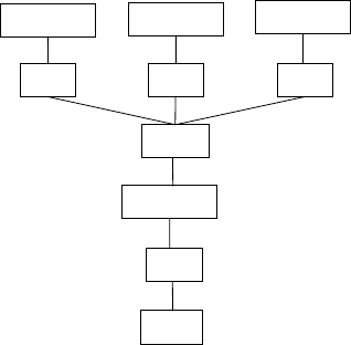
6.3 Index Rebuild 351
Sort
Fill index
Spool
Sort
Fill index
Sort
Fill index
Sort
Fill index
Scan
Fig. 6.4 Rebuilding primary index and secondary indexes.
Updating all existing secondary indexes might be slower than rebuilding
the indexes, partially because updates require full information in the
recovery log whereas rebuilding indexes can employ non-logged index
creation (allocation-only logging).
Figure 6.4 illustrates a query execution plan for rebuilding a table’s
primary index and subsequently its three secondary indexes. The scan
captures the data from the current primary index or heap file. The sort
prepares filling the new primary index. The spool operation retains
in temporary storage only those columns required for the secondary
indexes. The spool operation can be omitted if it is less expensive to
scan the new primary index repeatedly than to write and re-read the
spool data. Alternatively, the individual sort operations following the
spool operation can serve the purpose of the spool operation, as dis-
cussed earlier in connection with Figure 6.4.
In addition to non-logged index creation, index rebuild operations
can also employ other techniques from index creation such as partition-
ing, parallel execution, stitching B-trees with disjoint key ranges, etc.
For online index rebuild operations, the same techniques for locking,
anti-matter, etc. apply as for online index creation.
•
An index may be rebuild after a corruption (due to faulty
software or hardware) or when defragmentation is desired
but removing and rebuilding the index is faster.
352 B-tree Utilities
•
When a primary index is rebuilt, the secondary indexes usu-
ally must be rebuilt, too. Various optimizations apply to this
operation, including some that are usually not exploited for
standard query processing.
6.4 Bulk Insertions
Bulk insertion, also known as incremental load, roll-in, or information
capture, is a very frequent operation in many databases, in particular
data warehouses, data marts, and other databases holding informa-
tion about events or activities (such as sales transactions) rather than
states (such as account balances). Performance and scalability of bulk
insertions sometimes decides among competing vendors when the time
windows for nightly database maintenance or for the initial proof-of-
concept implementation are short.
Any analysis of performance or bandwidth of bulk insertions must
distinguish between instant bandwidth and sustained bandwidth, and
between online and offline load operations. The first difference is due
to deferred maintenance of materialized views, indexes, statistics such
as histograms, etc. For example, partitioned B-trees [43] enable high
instant load bandwidth (basically, appending to a B-tree at disk write
speed). Eventually, however, query performance deteriorates with addi-
tional partitions in each B-tree and requires reorganization by merging
partitions; such reorganization must be considered when determining
the load bandwidth that can be sustained indefinitely.
The second difference focuses on the ability to serve applications
with queries and updates during the load operation. For example, some
database vendors for some of their releases recommended dropping all
indexes prior to a large bulk insertion, say insertions larger than 1% of
the existing table size. This was due to the poor performance of index
insertions; rebuilding all indexes for 101% of the prior table size can be
faster than insertions equal to 1% of the table size.
Techniques optimized for efficient bulk insertions into B-trees can
be divided into two groups. Both groups rely on some form of buffering
to delay B-tree maintenance and to gain some economy of scale. The
first group focuses on the structure of B-trees and buffers insertions in

6.4 Bulk Insertions 353
branch nodes [74]. Thus, B-tree nodes are very large, are limited to a
small fan-out, or require additional storage “on the side.” The second
group exploits B-trees without modifications to their structure, either
by employing multiple B-trees [100] or by creating partitions within a
single B-tree by means of an artificial leading key field [43]. In all cases,
pages or partitions with active insertions are retained in the buffer pool.
The relative performance of the various methods, in particular in sus-
tained bandwidth, has not yet been investigated experimentally. Some
simple calculations below highlight the main effects on load bandwidth.
Figure 6.5 illustrates a B-tree node that buffers insertions, e.g., a
root node or a branch node. There are two separator keys (11 and 47),
three pointers to child nodes within the same B-tree, and a set of
buffered insertions with each child pointer. In a secondary index, index
entries contain a key value and reference to a record in the primary
index of the table, indicated by “ref” here. In other words, each buffered
insertion is a future leaf entry. The set of buffered insertions for the
middle child is much smaller than the one for the left child, perhaps
due to skew in the workload or a recent propagation of insertions to the
middle child. The set of changes buffered for the right child includes not
only insertions but also a deletion (key value 72). Buffering deletions
is viable only in secondary indexes, after a prior update of a primary
index has ensured that the value to be deleted indeed must exist in the
secondary index.
The essence of partitioned B-trees is to maintain partitions within a
single B-tree, by means of an artificial leading key field, and to reorga-
nize and optimize such a B-tree online using, effectively, the merge step
well known from external merge sort. This key field probably should
11 47
6, ref
7, ref
1, ref
17, ref
51, ref
72, ref
3, ref
63, ref
Fig. 6.5 Buffering in a branch node.

354 B-tree Utilities
be an integer of 2 or 4 bytes. By default, the same single value appears
in all records in a B-tree, and most of the techniques for partitioned
B-trees rely on exploiting multiple alternative values, temporarily in
most cases and permanently for a few techniques. If a table or view in
a relational database has multiple indexes, each index has its own arti-
ficial leading key field. The values in these fields are not coordinated
or propagated among the indexes. In other words, each artificial lead-
ing key field is internal to a single B-tree, such that each B-tree can
be reorganized and optimized independently of all others. If a table or
index is horizontally partitioned and represented in multiple B-trees,
the artificial leading key field should be defined separately for each
partition.
Figure 6.6 illustrates how the artificial leading key field divides the
records in a B-tree into partitions. Within each partition, the records
are sorted, indexed, and searchable by the user-defined key just as in a
standard B-tree. In this example partition 0 might be the main parti-
tion whereas partitions 3 and 4 contain recent insertions, appended to
the B-tree as new partitions after in-memory sorting. The last partition
might remain in the buffer pool, where it can absorb random insertions
very efficiently. When its size exceeds the available buffer pool, a new
partition is started and the prior one is written from the buffer pool to
disk, either by an explicit request or on demand during standard page
replacement in the buffer pool. Alternatively, an explicit sort operation
may sort a large set of insertions and then append one or multiple parti-
tions. The explicit sort really only performs run generation, appending
runs as partitions to the partitioned B-tree.
The initial load operation should copy the newly inserted records or
the newly filled pages into the recovery log such that the new database
3
4
Partition no. 0
Fig. 6.6 Partitions within a B-tree.
6.4 Bulk Insertions 355
contents is guaranteed even in the event of a media or system failure.
Reorganization of the B-tree can avoid logging the contents, and thus
log only the structural changes in the B-tree index, by careful write
ordering. Specifically, pages on which records or pointers have been
removed may over-write their earlier versions in their old location only
after new copies of the records have been written in their new location.
Minimal logging enabled by careful write ordering has been described
for other forms of B-tree reorganization [44, 89, 130] but it also applies
to merging in partitioned B-trees after bulk insertion by appending new
partitions.
For some example bandwidth calculations, consider bulk insertion
into a table with a primary index and three secondary indexes, all
stored on a single disk supporting 200 read–write operations per second
(100 read–write pairs) and 100 MB/s read–write bandwidth (assuming
large units of I/O and thus negligible access latency). In this example
calculation, record sizes are 1 KB in the primary index and 0.02 KB
in secondary indexes, including overheads for page and record head-
ers, free space, etc. For simplicity, let us assume a warm buffer pool
such that only leaf pages require I/O. The baseline plan relies on ran-
dom insertions into 4 indexes, each requiring one read and one write
operation. 8 I/Os per inserted row enable 25 row insertions per second
into this table. The sustained insertion bandwidth is 25 × 1KB=
25 KB/s = 0.025 MB/s per disk drive. This is both the instant and the
sustained insertion bandwidth.
For the plan relying on index removal and re-creation after insertion,
assume index removal is practically instant. With no indexes present,
the instant insertion bandwidth is equal to the disk write bandwidth.
After growing the table size by 1%, index creation must scan 101 times
the insertion volume, then write 106% of that data volume to run files
for the 4 indexes (sharing run generation when sorting for the secondary
indexes), and finally merge those runs into indexes: for a given amount
of data added, the I/O volume is 1 + 101 × (1+3× 1.06) = 423 times
that amount; at 100 MB/s, this permits 100/423 MB/s = 0.236 MB/s
sustained insertion bandwidth. While this might seem poor compared
to 100 MB/s, it is about ten times faster than random insertions, so it
is not surprising that vendors have recommended this scheme.
356 B-tree Utilities
For a B-tree implementation that buffers insertions at each branch
node, assume buffer space in each node for 10 times more insertions
than child pointers in the node. Propagation upon overflow focuses on
the child with the most pending insertions; let us assume that 20 records
can be propagated on average. Thus, only every 20th record insertion
forces reading and writing a B-tree leaf, or 1/20 of a read–write pair
per record insertion. On the other hand, B-tree nodes with buffer are
much larger and thus each record insertion might require reading and
writing both a leaf node and its parent, in which case each record inser-
tion forces 2/20=1/10 of a read–write pair. In the example table with
a primary index and three secondary indexes, i.e., 4 B-trees in total,
these assumptions lead to 4/10 of a read–write pair per inserted record.
The assumed disk hardware with 100 read–write pairs per second thus
support 250 record insertion per second or 0.250 MB/s sustained inser-
tion bandwidth. In addition to the slight bandwidth improvement when
compared to the prior method, this technique retains and maintains
the original B-tree indexes and permits query processing throughout
the load process.
With the assumed disk hardware, partitioned B-trees permit
100 MB/s instant insertion bandwidth, i.e., purely appending new
partitions sorted in the in-memory workspace using quicksort or
replacement selection. B-tree optimization, i.e., a single merge level
in a partitioned B-tree that reads and writes partitions, can process
50 MB/s. If reorganization is invoked when the added partitions reach
33% of the size of the master partition, adding a given amount of data
requires an equal amount of initial writing plus 4 times this amount
for reorganization (reading and writing). 9 amounts of I/O for each
amount of data produce a sustained insertion bandwidth of 11 MB/s
for a single B-tree. For the example table with a primary index and
three secondary indexes, this bandwidth must be divided among all
indexes, giving 11 MB/s ÷(1+3× 0.02) KB = 10 MB/s sustained
insertion bandwidth. This is more than an order of magnitude faster
than the other techniques for bulk loading. In addition, query pro-
cessing remains possible throughout initial capture of new informa-
tion and during B-tree reorganization. A multi-level merge scheme
might increase this bandwidth further because the master partition
6.5 Bulk Deletions 357
may be reorganized less often yet the number of existing partitions can
remain small.
In addition to traditional databases, B-tree indexes can also be
exploited for data streams. If only recent data items are to be retained
in the index, both bulk insertion techniques and bulk deletion tech-
niques are required. Therefore, indexing streams is discussed in the
next section.
•
Efficiency of bulk insertions (also known as load, roll-in, or
information capture) is crucial for database operations.
•
Efficiency of index maintenance is so poor in some imple-
mentations that indexes are removed prior to large load
operations. Various techniques have been published and
implemented to speed up bulk insertions into B-tree indexes.
Their sustained insertion bandwidths differ by orders of
magnitude.
6.5 Bulk Deletions
Bulk deletion, also known as purging, roll-out, or information
de-staging, can employ some of the techniques invented for bulk inser-
tion. For example, one technique for deletion simply inserts anti-matter
records with the fastest bulk insertion technique, leaving it to queries
or a subsequent reorganization to remove records and reclaim storage
space.
Partitioned B-trees permit reorganization prior to the actual dele-
tion. In the first and preparatory step, records to be deleted are moved
from the main “source” partition to a dedicated “victim” partition. In
the second and final step, this dedicated partition is deleted very effi-
ciently, mostly be simply de-allocation of leaf nodes and appropriate
repair of internal B-tree nodes. Note that the first step can be incre-
mental, rely entirely only system transactions, and can run prior to the
time when the information truly should vanish from the database.
Figure 6.7 shows the intermediate state of a partitioned B-tree
after preparation for bulk deletion. The B-tree entries to be deleted
have all been moved from the main partition into a separate parti-
tion such that their actual deletion and removal can de-allocate entire

358 B-tree Utilities
Partition no. 0 999
Fig. 6.7 Partitioned B-tree prepared for bulk deletion.
leaf pages rather than remove individual records distributed in all leaf
pages. If multiple future deletions can be anticipated, e.g., daily purge
of out-of-date information, multiple victim partitions can be populated
at the same time.
The log volume during bulk deletion in partitioned B-trees can
be optimized in multiple ways. First, the initial reorganization
(“un-merging”) into one or more victim partitions can employ the same
techniques as merging based on careful write ordering. Second, after the
victim partitions have been written back to the database, turning multi-
ple valid records into ghost records can be described in a single short log
record. Third, erasing ghost records does not require contents logging if
the log records for removal and commit are merged, as described earlier.
Fourth, de-allocation of entire B-tree nodes (pages) can employ simi-
lar techniques turning separator keys into ghost records. If the victim
partitions are so small that they can remain in the buffer pool until
their final deletion, committed deletion of pages in a victim partition
permits writing back dirty pages in the source partitions.
Techniques for bulk insertion and bulk deletion together enable
indexing of data streams. Data streaming and near-real-time data pro-
cessing can benefit from many database techniques, perhaps adapted,
e.g., from demand-driven execution to data-driven execution [22]. Most
stream management systems do not provide persistent indexes for
stream contents, however, because the na¨ıve or traditional index main-
tenance techniques would slow down processing rates too much.
With high-bandwidth insertions (appending partitions sorted in
memory), index optimization (merging runs), partition splitting (by
prospective deletion date), and deletions (by cutting entire partitions),
B-tree indexes on streams can be maintained even on permanent

6.6 Defragmentation 359
storage. For example, if a disk drive can move data at 100 MB/s, new
data can be appended, recent partitions merged, imminently obsolete
partitions split from the main partition, and truly obsolete partitions
cut at about 20 MB/s sustained. If initial or intermediate partitions are
placed on particularly efficient storage, e.g., flash devices or nonvolatile
RAM, or if devices are arranged in arrays, the system bandwidth can
be much higher.
A stream with multiple independent indexes enables efficient inser-
tion of new data and concurrent removal of obsolete data even if mul-
tiple indexes require constant maintenance. In that case, synchronizing
all required activities imposes some overhead. Nonetheless, the example
disk drive can absorb and purge index entries (for all indexes together)
at 20 MB/s.
Similar techniques enable staging data in multiple levels of a
storage hierarchy, e.g., in-memory storage, flash devices, performance-
optimized “enterprise” disks and capacity-optimized “consumer” disks.
Disk storage may differ not only in the drive technology but also in the
approach to redundancy and failure resilience. For example, perfor-
mance is optimized with a RAID-1 “mirroring” configuration whereas
cost-per-capacity is optimized with a RAID-5 “striped redundancy”
configuration or a RAID-6 “dual redundancy” configuration. Note that
RAID-5 and -6 can equal each other in cost-per-capacity because the
latter can tolerate dual failures and thus can be employed in larger disk
arrays.
•
Bulk deletion is less important than bulk insertion; nonethe-
less, various optimizations can affect bandwidth by orders of
magnitude.
•
Indexing data streams requires techniques from both bulk
insertion and bulk deletion.
6.6 Defragmentation
1
Defragmentation in file systems usually means placing blocks phys-
ically together that belong to the same file; in database B-trees,
1
Much material in this section is copied from [55].
360 B-tree Utilities
defragmentation encompasses a few more considerations. These con-
siderations apply to individual B-tree nodes or pages, to the B-tree
structure, and to separator keys. In many cases, defragmentation logic
can be invoked when some or all affected pages are in the buffer pool
due to normal workload processing, resulting in incremental and online
defragmentation or reorganization [130].
For each node, defragmentation includes free space consolidation
within each page for efficient future insertions, removal of ghost records
(unless currently locked by user transactions), and optimization of in-
page data compression (e.g., de-duplication of field values). The B-tree
structure might be optimized by defragmentation for balanced space
utilization, free space as discussed above in the context of B-tree cre-
ation, shorter separator keys (suffix truncation), and better prefix trun-
cation on each page.
B-tree defragmentation can proceed in key order or in independent
key ranges, which also creates an opportunity for parallelism. The key
ranges for each task can be determined a priori or dynamically. For
example, when system load increases, a defragmentation task can com-
mit its changes instantaneously, pause, and resume later. Note that
defragmentation does not change the contents of a B-tree, only its
representation. Therefore, the defragmentation task does not need to
acquire locks. It must, of course, acquire latches to protect in-memory
data structures such as page images in the buffer pool.
Moving a node in a traditional B-tree structure is quite expensive,
for several reasons. First, the page contents might be copied from one
page frame within the buffer pool to another. While the cost of doing
so is moderate, it is probably faster to “rename” a buffer page, i.e., to
allocate and latch buffer descriptors for both the old and new locations
and then to transfer the page frame from one descriptor to the other.
Thus, the page should migrate within the buffer pool “by reference”
rather than “by value.” If each page contains its intended disk location
to aid database consistency checks, this field must be updated at this
point. If it is possible that a de-allocated page lingers in the buffer
pool, e.g., after a temporary table has been created, written, read,
and dropped, this optimized buffer operation must first remove from
the buffer’s hash table any prior page with the new page identifier.
6.6 Defragmentation 361
Alternatively, the two buffer descriptors can simply swap their two
page frames.
Second, moving a page can be expensive because each B-tree node
participates in a web of pointers. When moving a leaf page, the parent
as well as both the preceding leaf and the succeeding leaf must be
updated. Thus, all three surrounding pages must be present in the
buffer pool, their changes recorded in the recovery log, and the modified
pages written to disk before or during the next checkpoint. It is often
advantageous to move multiple leaf pages at the same time, such that
each leaf is read and written only once. Nonetheless, each single-page
move operation can be a single system transaction, such that locks
can be released frequently both for the allocation information (e.g., an
allocation bitmap) and for the index being reorganized.
If B-tree nodes within each level do not form a chain by physical
page identifiers, i.e., if each B-tree node is pointed to only by its parent
node but not by neighbor nodes, page migration and therefore defrag-
mentation are considerably less expensive. Specifically, only the parent
of a B-tree node requires updating when a page moves. Neither its
siblings nor its children are affected; they are not required in memory
during a page migration, they do not require I/O or changes or log
records, etc.
The third reason why page migration can be quite expensive is
logging, i.e., the amount of information written to the recovery log.
The standard, “fully logged” method to log a page migration during
defragmentation is to log the page contents as part of allocating and
formatting a new page. Recovery from a system crash or from media
failure unconditionally copies the page contents from the log record to
the page on disk, as it does for all other page allocations.
Logging the entire page contents is only one of several means
to make the migration durable, however. A second, “forced write”
approach is to log the migration itself with a small log record that
contains the old and new page locations but not the page contents, and
to force the data page to disk at the new location prior committing the
page migration. Forcing updated data pages to disk prior to transac-
tion commit is well established in the theory and practice of logging and
recovery [67]. A recovery from a system crash can safely assume that a
362 B-tree Utilities
committed migration is reflected on disk. Media recovery, on the other
hand, must repeat the page migration, and is able to do so because the
old page location still contains the correct contents at this point during
log-driven redo. The same applies to log shipping and database mir-
roring, i.e., techniques to keep a second (often remote) database ready
for instant failover by continuously shipping the recovery log from the
primary site and running continuous redo recovery on the secondary
site.
The most ambitious and efficient defragmentation method neither
logs the page contents nor forces it to disk at the new location. Instead,
this “non-logged” page migration relies on the old page location to pre-
serve a page image upon which recovery can be based. During system
recovery, the old page location is inspected. If it contains a log sequence
number lower than the migration log record, the migration must be
repeated, i.e., after the old page has been recovered to the time of the
migration, the page must again be renamed in the buffer pool, and
then additional log records can be applied to the new page. To guaran-
tee the ability to recover from a failure, it is necessary to preserve the
old page image at the old location until a new image is written to the
new location. Even if, after the migration transaction commits, a sep-
arate transaction allocates the old location for a new purpose, the old
location must not be overwritten on disk until the migrated page has
been written successfully to the new location. Thus, if system recovery
finds a newer log sequence number in the old page location, it may
safely assume that the migrated page contents are available at the new
location, and no further recovery action is required.
Some methods for recoverable B-tree maintenance already employ
this kind of write dependency between data pages in the buffer pool, in
addition to the well-known write dependency of write-ahead logging. To
implement this dependency using the standard technique, both the old
and new page must be represented in the buffer manager. Differently
than in the usual cases of write dependencies, the old location may be
marked clean by the migration transaction, i.e., it is not required to
write anything back to the old location on disk. Note that redo recovery
of a migration transaction must re-create this write dependency, e.g.,
in media recovery and in log shipping.
6.6 Defragmentation 363
The potential weakness of this third method are backup and restore
operations, specifically if the backup is “online,” i.e., taken while the
system is actively processing user transactions, and the backup con-
tains not the entire database but only pages currently allocated to
some table or index. Moreover, the detailed actions of the backup pro-
cess and page migration must interleave in a particularly unfortunate
way. In this case, a backup might not include the page image at the
old location, because it is already de-allocated. Thus, when backing up
the log to complement the online database backup, migration transac-
tions must be complemented by the new page image. In effect, in an
online database backup and its corresponding restore operation, the
logging and recovery behavior is changed in effect from a non-logged
page migration to a fully logged page migration. Applying this log dur-
ing a restore operation must retrieve the page contents added to the
migration log record and write it to its new location. If the page also
reflects subsequent changes that happened after the page migration,
recovery will process those changes correctly due to the log sequence
number on the page. Again, this is quite similar to existing mechanisms,
in this case the backup and recovery of “non-logged” index creation
supported by some commercial database management systems.
While a migration transaction moves a page from its old to its new
locations, it is acceptable for a user transaction to hold a lock on a key
within the B-tree node. It is necessary, however, that any such user
transaction must search again for the B-tree node, with a new search
pass from B-tree root to leaf, in order to obtain the new page identifier
and to log further contents changes, if any, correctly. This is very similar
to split and merge operations of B-tree nodes, which also invalidate
knowledge of page identifiers that user transactions may temporarily
retain. Finally, if a user transaction must roll back, it must compensate
its actions at the new location, again very similarly to compensating a
user transaction after a different transaction has split or merged B-tree
nodes.
•
Most implementations of B-trees (as of other storage struc-
tures) require occasional defragmentation (reorganization) to
ensure contiguity (for fewer seeks during scans), free space,
etc.

364 B-tree Utilities
•
The cost of page movement can be reduced by using fence
keys instead of neighbor pointers (see also Sections 3.5 and
4.4) and by careful write ordering (see also Section 4.10).
•
Defragmentation (reorganization, compaction) can proceed
in many small system transactions and it can ‘pause and
resume’ without wasting work.
6.7 Index Verification
2
There obviously is a large variety of techniques for efficient data
structures and algorithms for B-tree indexes. As more techniques are
invented or implemented in a specific software system, omissions or
mistakes occur and must be found. Many of these mistakes mani-
fest themselves in data structures that do not satisfy the intended
invariants. Thus, as part of rigorous regression testing during software
development and improvement, verification of B-trees is a crucial
necessity.
Many of these omissions and mistakes require large B-trees, high
update and query loads, and frequent verification in order to be found
in a timely manner during software development. Thus, efficiency is
important in B-tree verification.
To be sure, verification of B-trees is also needed after deployment.
Hardware defects occur in DRAM, flash devices, and disk devices as is
well known [114]. Software defects can be found not only in database
management systems but also in device drivers, file system code, etc.
[5, 61]. While some self-checking exists in many hardware and software
layers, vendors of database management system recommend regular
verification of databases. Verification of backup media is also valuable
as it enhances the trust and confidence is those media and their con-
tents, should they ever be needed.
For example, Mohan described the danger of partial writes due
to performance optimizations in implementations of the SCSI stan-
dard [94]. His focus was on problem prevention using appropriate
page modification, page verification after each read operation, logging,
2
Much of this section is derived from [54].

6.7 Index Verification 365
c b
a
d
Fig. 6.8 An incomplete leaf split.
log analysis, recovery logic, etc. The complexity of these techniques,
together with the need for ongoing improvements in these performance-
critical modules, reinforces our belief that complete, reliable, and effi-
cient verification of B-tree structures is a required defensive measure.
For example, Figure 6.8 shows the result of an incorrect splitting of
a leaf node. When leaf node b was split and leaf node c was created, the
backward pointer in successor node d incorrectly remained unchanged.
A subsequent (descending) scan of the leaf level will produce a wrong
query result, and subsequent split and merge operations will create fur-
ther havoc. The problem might arise after an incomplete execution, an
incomplete recovery, or an incomplete replication of the split opera-
tion. The cause might be a defect in the database software, e.g., in the
buffer pool management, or in the storage management software, e.g.,
in snapshot or version management. In other words, there are many
thousands of lines of code that may contain a defect that leads to a
situation like the one illustrated in Figure 6.8.
As B-trees are complex data structures, efficient verification off all
invariants has long been elusive, including in-page invariants, parent-
child pointers and neighbor pointers, and key relationships, i.e., the
correct ordering of separator keys and keys in the leaf nodes. The
latter problem pertains not only to parent-child relationships but to
all ancestor-descendent relationships. For example, a separator key in
a B-tree’s root node must sort not only the keys in the root’s immedi-
ate children but keys at all B-tree levels down to the leaves. Invariants
that relate multiple B-trees, e.g., the primary index of a table and its
secondary indexes or a materialized view and its underlying tables and
views, can usually be processed with appropriate joins. If all aspects of
database verification are modeled as query processing problems, many
query processing techniques can be exploited, from resource manage-
ment to parallel execution.

366 B-tree Utilities
In-page invariants are easy to validate once a page is in the buffer
pool but exhaustive verification requires checking all instances of all
invariants, e.g., key range relationships between all neighboring leaf
nodes. The cross-page invariants are easy to verify with an index-order
sweep over the entire key range. If, however, an index-order sweep is
not desirable due to parallel execution or due to the limitations of
backup media such as tapes, the structural invariants can be verified
using algorithms based on aggregation. While scanning B-tree pages
in any order, required information is extracted from each page and
matched with information from other pages. For example, neighbor
pointers match if page x names page y as its successor and page y
names page x as its predecessor. Key ranges must be included in the
extracted information in order to ensure that key ranges are disjoint
and correctly distinguished by the separator key in the appropriate
ancestor node. If two leaf nodes share a parent node, this test is quite
straightforward; if the lowest common ancestor is further up in the
B-tree, and if transitive operations are to be avoided, some additional
information must be retained in B-tree nodes.
Figure 6.9 shows a B-tree with neighboring leaf nodes with no shared
parent but instead a shared grandparent, i.e., cousin nodes d and e.
Shaded areas represent records and their keys; two keys are different
(equal) if their shading is different (equal). Efficient verification of keys
and pointers among cousin nodes d and e does not have an immediate
or obvious efficient solution in a traditional B-tree implementation. The
potential problem is that there is no easy way to verify that all keys
Fig. 6.9 The cousin problem in B-tree verification.

6.7 Index Verification 367
Fig. 6.10 Fence keys and cousin nodes.
in leaf page d are indeed smaller than the separator key in root page
a and that all keys in leaf page e are indeed larger than the separator
key in root page a. Correct key relationships between neighbors (b−c
and d−e) and between parents and children (a−b,a−c, b−d,c−e)donot
guarantee correct key relationships across skipped levels (a−d,a−e).
Figure 6.10 shows how fence keys enable a simple solution for the
cousin problem in B-tree verification, even if fence keys were originally
motivated by write-optimized B-trees [44]. The essential difference to
traditional B-tree designs is that page splits not only post a separator
key to the parent page but also retain copies of this separator key as
high and low “fence keys” in the two post-split sibling pages. Note that
separators and thus fence keys can be very short due to prefix and
suffix truncation [10]. These fence keys take the role of sibling pointers,
replacing the traditional page identifiers with search keys. Fence keys
speed up defragmentation by eliminating all but one page identifier
that must be updated when a page moves, namely the child pointer
in the parent node. Fence keys also assist key range locking since they
are key values that can be locked. In that sense, they are similar to
traditional ghost records, except that fence keys are not subject to ghost
cleanup.
The important benefit here is that verification is simplified and
the cousin problem can readily be solved, including “second cousins,”
“third cousins,” etc. in B-trees with additional levels. In Figure 6.10,
the following four pairs of facts can be derived about the key marked
368 B-tree Utilities
by horizontal shading, each pair derived independently from two
pages.
1. From page a, the fact that b is a level-1 page, and its high
fence key
2. From page a, the fact that c is a level-1 page, and its low
fence key
3. From page b, the fact that b is a level-1 page, and its high
fence key; this matches fact 1 above
4. From page b, the fact that d is a leaf page, and its high fence
key
5. From page c, the fact that c is a level-1 page, and its low
fence key; this matches fact 2 above
6. From page c, the fact that e is a leaf page, and its low fence
key
7. From page d, the fact that d is a leaf page, and its high fence
key; this matches fact 4 above
8. From page e, the fact that e is a leaf page, and its low fence
key; this matches fact 6 above
No match is required between cousin pages d and e. Their fence
keys are equal due to transitivity among the other comparisons. In
fact, matching facts derived from pages d and e could not include page
identifiers, because these pages do not carry the other’s page identifiers.
At best, the following facts could be derived, although they are implied
by the ones above and thus do not contribute to the quality of B-tree
verification:
9. From page b, the fact that a level-1 page has a specific high
fence key
10. From page c, the fact that a level-1 page has a specific low
fence key; to match fact 9 above
11. From page d, the fact that a leaf page has a specific high
fence key
12. From page e, the fact that a leaf page has a specific low
fence key; to match fact 11 above
6.7 Index Verification 369
The separator key from the root is replicated along the entire seam
of neighboring nodes all the way to the leaf level. Equality and con-
sistency are checked along the entire seam and, by transitivity, across
the seam. Thus, fence keys also solve the problem of second and third
cousins etc. in B-trees with additional levels.
These facts can be derived in any order; thus, B-tree verification can
consume database pages from a disk-order scan or even from backup
media. These facts can be matched using an in-memory hash table
(and possibly hash table overflow to partition files on disk) or they can
be used to toggle bits in a bitmap. The former method requires more
memory and more CPU effort but can identify any error immediately;
the latter method is faster and requires less memory, but requires a
second pass of the database in case some facts fail to match equal facts
derived from other pages. Moreover, the bitmap method has a miniscule
probability of failing to detect two errors that mask each other.
Fence keys also extend local online verification techniques [80]. In
traditional systems, neighbor pointers can be verified during a root-to-
leaf navigation only for siblings but not for cousins, because the iden-
tity of siblings is known from information in the shared parent node
but verification of a cousin pointer would require an I/O operation to
fetch the cousin’s parent node (also its grandparent node for a second
cousin, etc.). Thus, earlier techniques [80] cannot verify all correctness
constraints in a B-tree, no matter how many search operations per-
form verification. Fence keys, on the other hand, are equal along entire
B-tree seams, from leaf level to the ancestor node where the key value
serves as separator key. A fence key value can be exploited for online
verification at each level in a B-tree, and an ordinary root-to-leaf B-tree
descent during query and update processing can verify not only siblings
with a shared parent but also cousins, second cousins, etc. Two search
operations for keys in neighboring leaves verify all B-tree constraints,
even if the leaves are cousin nodes, and search operations touching all
leaf nodes verify all correctness constraints in the entire B-tree.
For example, two root-to-leaf searches in the index shown in
Figure 6.10 may end in leaf nodes d and e. Assume that these two
root-to-leaf passes occur in separate transactions. Those two searches
can verify correct fence keys along the entire seam. In the B-tree
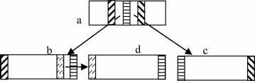
370 B-tree Utilities
that employs neighbor pointers rather than fence keys as shown in
Figure 6.9, the same two root-to-leaf searches could verify that entries
in leaf nodes d and e are indeed smaller and larger than the separator
key in the root node but they cannot verify that the pointers between
cousin nodes d and e are mutual and consistent.
B-tree verification by extracting and matching facts applies not
only to traditional B-trees but also to B
link
-trees and their transi-
tional states. Immediately after a node split, the parent node is not yet
updated in B
link
-tree and thus generates the facts as above. The newly
allocated page is a normal page and also generates the facts as above.
The page recently split is the only one with special information, namely
a neighbor pointer. Thus, a page with a neighbor pointer indicating a
recent split not yet reflected in the parent must trigger derivation of
some special facts. Since this old node provides the appropriate “parent
facts” for the new node, the old node could be called a “foster parent”
if one wants to continue the metaphor of parent, child, ancestor, etc.
Figure 6.11 illustrates such a case, with node b recently split. The
fact about the low fence key of node d cannot be derived from the
(future) parent node a. The fact derived from node d must be matched
by a fact derived from node b. Thus, node b acts like a temporary parent
for the new node d not only in terms of the search logic but also during
verification of the B-tree structure. Note that the intermediate state in
Figure 6.11 could also be used during node removal from a B-tree, again
with the ability to perform complete and correct B-tree verification at
any time, in any sequence of nodes, and thus on any media.
In addition to verification of a B-tree structure, each individual
page must be verified prior to extraction of facts, and multiple B-tree
indexes may need to be matched against one another, e.g., a secondary
index against the appropriate identifier in the primary index. In-page
Fig. 6.11 Fence keys and verification in a B
link
-tree.
6.8 Summary 371
verification is fairly straightforward, although it might be surprising
how many details are worth validating. Matching multiple indexes
against one another is very similar to a join operation and all stan-
dard join algorithms can be employed. Alternatively, a bitmap can be
used, with a miniscule probability of two errors masking each other and
with a second pass required if the bitmap indicates that an error exists.
Automatic repair of B-tree indexes is not well studied. Techniques
may rely on dropping and rebuilding an entire index, replaying the
recovery log for just one page, or adjusting a page to match its related
pages. A systematic study of repair algorithms, their capabilities, and
their performance would be useful for the entire industry.
•
Verification of B-tree indexes protects against software and
hardware faults. All commercial database systems provide
such utilities.
•
B-trees can be verified by a single index-order scan, which
may be expensive due to fragmentation.
•
Verification based on a disk-order scan requires aggregation
of facts extracted from pages. A bit vector filter can speed the
process but, in case an inconsistency is found, cannot identify
the inconsistency precisely (due to possible hash collisions).
•
Query execution may (as a side effect) verify all B-tree invari-
ants if nodes carry fence keys rather than neighbor pointers.
6.8 Summary
In summary, utilities play an important role in the usability and total
cost of ownership of database systems. B-trees are unique among index
structures because a large number of techniques for efficient utilities are
well known and widely implemented. Newly proposed index structures
must compete with B-trees for performance and scalability not only
during query processing and updates but also during utility operations
from index creation to defragmentation and index verification.

7
Advanced Key Structures
As the prior sections have demonstrated, a large amount of planning
and coding is required in order to fully support database index struc-
tures such as B-trees. No other index structure has received as much
attention from database researchers and software developers. By careful
and creative construction of B-tree keys, however, additional indexing
capabilities can be enabled with few, if any, modifications within the
core B-tree code. The present section surveys several of them.
The present section does not consider indexes on computed columns,
i.e., values derived from other columns in the same table and given a
name in the database schema. These columns are computed as needed
and need not be stored in the main data structure for the table. If there
is an index on such a column, however, appropriate key values are stored
in this secondary index.
Similarly, the present section does not consider partial indexes, i.e.,
indexes with fewer entries than rows in the underlying table based
on a selection predicate. A typical predicate ensures that only values
other than Null are indexed. Both topics, computed columns and partial
indexes, are orthogonal to advanced key structures in B-trees.
372
7.1 Multi-dimensional UB-trees 373
An earlier discussion (Section 2.5) gave an example of unusual
B-tree keys, namely hash indexes implemented as B-trees on hash
values. A few small adaptations in the B-tree code emulate the
main performance benefits traditionally associated with hash indexes,
namely a single I/O in the worst case, direct address calculation within
the hash directory, and efficient key value comparisons. The first can
be emulated with a very large root page pinned in the buffer pool
(very similar to a large hash directory); the other two benefits can be
mirrored by appropriate key values including poor man’s normalized
keys.
•
B-trees with advanced key structures retain all the advan-
tages of B-trees, e.g., theory and implementation of key range
locking, optimizations of logging and recovery, efficient index
creation, and other utilities for efficient database operations.
•
A B-tree on hash values has many advantages over a tradi-
tional hash index with comparable performance.
7.1 Multi-dimensional UB-trees
By their nature, B-trees support only a single sort order. If multiple key
columns are used, they may form a hierarchy of major sort key, minor
sort key, etc. In this case, queries that restrict the leading key columns
perform better than those that do not. If, however, the key columns
represent dimensions in a space, e.g., a geometric space, queries may
restrict the leading column only by a range predicate or not at all.
Leslie et al. [82] describe sophisticated algorithms for accessing B-trees
in those cases.
An alternative approach projects multi-dimensional data onto a sin-
gle dimension based on space-filling curves. The principal tradeoff in the
design of space-filling curves is conceptual and computational simplic-
ity on one hand and preservation of locality and thus search efficiency
on the other hand. The simplest construction of a space-filling curve
first maps each dimension into an unsigned integer and then inter-
leaves individual bits from these integers. When drawn as a line in a
2-dimensional space, this space-filling curve resembles nested Z shapes,
which is why it is also called the z-order. This is the design underlying

374 Advanced Key Structures
Fig. 7.1 Z-order curves.
multi-dimensional indexing and query processing in Probe [106] and
Transbase [109]. Alternatives to this Morton curve include the Hilbert
curve and others.
Figure 7.1 (copied from [106]) illustrates z-order curves. The origi-
nal x- and y-coordinates have 3 bits and therefore 8 distinct values; the
interleaved z-values contain 6 bits and therefore 64 points. The “Z”
shape is repeated at 3 scales. The technique applies to any number of
dimensions, not only 2-dimensional spaces as shown in Figure 7.1.
UB-trees are B-tree indexes on such z-values. Each point and range
query against the original dimensions is mapped to the appropriate
intervals along the z-curve. The crucial component of this mapping
is determining the z-values at which the z-curve enters and exits the
multi-dimensional range defined by the query predicate. Known algo-
rithms are linear in the number of original dimensions, their resolution
(i.e., the number of bits in the z-values), and the number of entry and
exit points [109].
In addition to points in multi-dimensional space, space-filling
curves, z-order mappings, and UB-trees can index multi-dimensional
rectangles (boxes) by treating start and end points as separate dimen-
sions. In other words, UB-trees can index not only information about
points but also about intervals and rectangles. Both space and time
(including intervals) can be indexed in this way. For moving objects,
location and speed (in each spatial dimension) can be treated as

7.2 Partitioned B-trees 375
separate dimensions. Finally, even precision in location or speed can
be indexed, if desired. Unfortunately, indexing based on space-filling
curves loses effectiveness with the number of dimensions, just as the
performance of traditional B-tree applications suffers when a B-tree
contains many columns but only a few of them are specified in a query
predicate.
•
Z-values (or other space-filling curves) provide some multi-
dimensional indexing with all the advantages of B-trees.
•
The query performance of specialized multi-dimensional
indexes is probably better, but load and update performance
of B-trees are not easy to match.
7.2 Partitioned B-trees
As discussed earlier in the section on bulk insertions and illustrated
in Figure 6.6, the essence of partitioned B-trees [43]
1
is to maintain
partitions within a single B-tree, by means of an artificial leading key
field. Partitions and the artificial leading key field are hidden from the
database user. They exist in order to speed up large operations on
B-trees, not to carry any information. Partitions are optimized using
the merge step well known from external merge sort. By default, the
same single value appears in all records in a B-tree, and most of the
specific techniques rely on exploiting multiple alternative values, but
only temporarily. If a table or index is represented in multiple B-trees,
the artificial leading key field should be defined separately for each such
B-tree.
The leading artificial key column effectively defines partitions within
a single B-tree. Each existing distinct value implicitly defines a par-
tition, and partitions appear and vanish automatically as records are
inserted and deleted. The design differs from traditional horizontal par-
titioning using a separate B-tree for each partition in an important
way: Most advantages of the design depend on partitions (or distinct
values in the leading artificial key column) being created and removed
very dynamically. In a traditional implementation of partitioning (using
1
The text in this subsection is adapted from this reference.
376 Advanced Key Structures
multiple B-trees), creation or removal of a partition is a change of the
table’s schema and catalog entries, which requires locks on the table’s
schema or catalog entries and thus excludes concurrent or long-running
user accesses to the table, as well as forcing recompilation of cached
query and update plans. If partitions within a single B-tree are created
and removed as easily as inserting and deleting rows, smooth contin-
uous operation is relatively easy to achieve. It is surprising how many
problems this simple technique can help address in data management
software and its real-world usage.
First, it permits putting all runs in an external merge sort into
a single B-tree (with the run number as the artificial leading key
field), which in turn permits improvements to asynchronous read-ahead
and to adaptive memory usage. In SAN and NAS environments, hid-
ing latency by exploiting asynchronous read-ahead is important. With
striped disks, forecasting multiple I/O operations is important. Finally,
in very large online databases, the ability to dynamically grow and
shrink resources dedicated to a single operation is very important, and
the proposed changes permit doing so even to the extremes of pausing
an operation altogether and of letting a single operation use a machine’s
entire memory and entire set of processors during an otherwise idle
batch window. While sorting is used to build B-tree indexes efficiently
and B-trees are used to avoid the expense of sorting and to reduce the
expense of searching during query processing, the mutually beneficial
relationship between sorting and B-trees can go substantially further.
Second, partitioned B-trees can substantially reduce, by at least a
factor of two, the wait time before a newly created index is available for
query answering. While the initial form of an index does not perform
as well as the final, fully optimized index or a traditional index, at
least it is usable by queries and permits replacing table scans with
index searches, resulting in better query response time as well as a
smaller “locking footprint” and thus a reduced likelihood of deadlocks.
Moreover, the index can be improved incrementally from its initial form
to its final and fully optimized form, which is very similar to the final
form after traditional index creation. Thus, the final index is extremely
similar in performance to indexes created offline or with traditional
online methods; the main difference is cutting in half (or better) the
7.2 Partitioned B-trees 377
delay between a decision to create a new index and its first beneficial
impact on query processing.
Third, adding a large amount of data to a large, fully indexed
data warehouse so far has created a dilemma between dropping and
rebuilding all indexes or updating all indexes one record at a time,
implying random insertions, poor performance, a large log volume, and
a large incremental backup. Partitioned B-trees resolve this dilemma
in most cases without special new data structures. A load operation
simply appends a number of new partitions to each affected index; the
size of these partitions is governed by the memory allocation for the
in-memory run generation during the load operation. Updates (both
insertion and deletions) can be appended to an existing B-tree in one or
multiple new partitions, to be integrated into the main partition at the
earliest convenient time, at which time deletions can be applied to the
appropriate old records. Appending partitions is, of course, yet another
variation on the theme of differential files [117]. Batched maintenance
in a partitioned B-tree reduces the overall update time; in addition, it
can improve the overall space requirements if pages of the main parti-
tion are filled completely with compressed records; and it may reduce
query execution times if the main partition remains unfragmented and
its pages optimized for efficient search, e.g., interpolation search.
While a partitioned B-tree actually contains multiple partitions, any
query must search all of them. It is unlikely (and probably not even per-
mitted by the query syntax) that a user query limits itself to a subset of
partitions or even a single one. On the other hand, a historic or “as of”
query might map to a single partition even when newer partitions are
already available. In general, however, all existing partitions must be
searched. As partitioning is implemented with an artificial leading key
field in an otherwise standard B-tree implementation, this is equivalent
to a query failing to restrict the leading column in a traditional multi-
column B-tree index. Efficient techniques for this situation are known
and not discussed further here [82].
Partitions may remain as initially saved or they may be merged.
Merging may be eager (e.g., merging as soon as the number of parti-
tions reaches a threshold), opportunistic (e.g., merging whenever there
is idle time), or lazy (e.g., merging key ranges required to answer actual
378 Advanced Key Structures
queries). The latter is called adaptive merging [53]. Rather than merg-
ing partitions in preparation of query processing, merging can be inte-
grated into query execution, i.e., be a side effect of query execution.
Thus, even if key ranges are left as parameters in query predicates, this
technique merges only key ranges actually queried. All other key ranges
remain in the initial partitions. No merge effort is spent on them yet
they are ready for query execution and index optimization should the
workload and its access pattern change over time.
•
In partitioned B-trees, partitions are identified by an artificial
leading key field. Partitions appear and disappear simply by
insertion and deletion of B-tree entries with appropriate key
values, without catalog updates.
•
Partitioned B-trees are useful for efficient sorting (e.g., deep
read-ahead), index creation (e.g., early query processing),
bulk insertion (append-only data capture with in-memory
sorting), and bulk deletion (victim preparation).
•
Query performance equals that of traditional B-trees once all
partitions have been merged, which is the default state.
7.3 Merged Indexes
As others have observed, “optimization techniques that reduce the
number of physical I/Os are generally more effective than those that
improve the efficiency in performing the I/Os” [70]. It is a common
belief that clustering related records requires pointers between records.
An example relational database management system with record clus-
tering is Starburst [20], which uses hidden pointers between related
records and affects their automatic maintenance during insertions, dele-
tions, and updates. The technique serves only tables and their primary
storage structures, not secondary indexes, and it requires many-to-one
relationships defined with foreign key integrity constraints.
The desirability of clustering secondary indexes is easily seen in
a many-to-many relationship such as “enrollment” as many-to-many
relationship between “courses” and “students.” In order to support
table-to-table, index-to-index, and record-to-record navigation both
from students to courses and from courses to students, the enrollment

7.3 Merged Indexes 379
table requires at least two indexes, only one of which can be the primary
index. For efficient data access in both directions, however, it would be
desirable to cluster one enrollment index with student records and one
enrollment index with course records.
Merged indexes [49]
2
are B-trees that contain multiple traditional
indexes and interleave their records based on a common sort order.
In relational databases, merged indexes implement “master-detail
clustering” of related records, e.g., orders and order details. Thus,
merged indexes shift de-normalization from the logical level of tables
and rows to the physical level of indexes and records, which is a more
appropriate place for it. For object-oriented applications, clustering can
reduce the I/O cost for joining rows in related tables to a fraction com-
pared to traditional indexes, with additional beneficial effects on buffer
pool requirements.
Figure 7.2 shows the sort order of records within such a B-tree. The
sort order alone keeps related records co-located; no additional point-
ers between records are needed. In its most limited form, master-detail
clustering combines two secondary indexes, e.g., associating two lists
of row identifiers with each key value. Alternatively, master-detail clus-
tering may merge two primary indexes but not admit any secondary
indexes. The design for merged indexes accommodates any combination
of primary and secondary indexes in a single B-tree, thus enabling clus-
tering of entire complex objects. Moreover, the set of tables, views, and
indexes can evolve without restriction. The set of clustering columns
can also evolve freely. A relational query processor can search and
Order 4711, Customer “Smith”, …
Order 4711, Line 1, Quantity 3, …
Order 4711, Line 2, Quantity 1, …
Order 4711, Line 3, Quantity 9, …
Order 4712, Customer “Jones”, …
Order 4712, Line 1, Quantity 1, …
…
…
Fig. 7.2 Record sequence in a merged index.
2
The text of this subsection is adapted from this reference.

380 Advanced Key Structures
update index records just as in traditional indexes. With these abilities,
the proposed design may finally bring general master-detail clustering
to traditional databases together with its advantages in performance
and cost.
In order to simplify design and implementation of merged indexes, a
crucial first step is to separate implementation of the B-tree structure
from its contents. One technique is to employ normalized keys, dis-
cussed and illustrated earlier in Figure 3.4, such that the B-tree struc-
ture manages only binary records and binary keys. In merged indexes,
the mapping from multi-column keys to binary search keys in a B-tree
is a bit more complex than in traditional indexes, in particular if adding
and removing any index at any time is desired and if individual indexes
may have different key columns. Thus, it is essential to design a flex-
ible mapping from keys in the index to byte strings in the B-tree. A
tag that indicates a key column’s domain and precedes the actual key
fields, as shown in Figure 7.3, can easily achieve this. In other words,
when constructing a normalized key for a merged index, domain tags
and field values alternate up to and including the identifier for the
index.
In practice, different than illustrated in Figure 7.3, a domain tag
will be a small number, not a string. It is possible to combine the
domain tag with the Null indicator (omitted in Figure 7.3) such that
the desired sort order is achieved yet actual values are stored on byte
boundaries. Similarly, the index identifier will be a number rather than
a string.
FIELD VALUE FIELD TYPE
“Customer identifier” Domain tag
123 Data value
“Order number” Domain tag
4711 Data value
“Index identifier” Domain tag
“Orders.OrderKey” Identifier value
“2006/12/20” Data value
“Urgent” Data value
… Data values
Fig. 7.3 B-tree record in a merged index.

7.4 Column Stores 381
Domain tags are not required for all fields in a B-tree record. They
are needed only for key columns, and more specifically only for those
leading key columns needed for clustering within the merged index.
Following these leading key columns is a special tag and the identifier
of the individual index to which the record belongs. For example, in
Figure 7.3, there are only 2 domain tags for key values plus the index
identifier. If there never will be any need to cluster on the line numbers
in order details, only leading key fields up to order number require the
domain tag. Thus, the per-record storage overhead for merged indexes
is small and may indeed be hidden in the alignment of fields to word
boundaries for fast in-memory processing. An overhead of 2–4 single-
byte domain tags per record may prove typical in practice.
•
Merging multiple indexes into a single B-tree provides
master-detail clustering with all the advantages of B-trees.
A single B-tree may contain any number of primary and sec-
ondary indexes of any number of tables.
•
The B-tree key alternates domain tags and values up to and
including the index identifier.
•
Merged indexes permit tables in traditional normal forms
with the performance of free denormalization.
•
Merged indexes are particularly valuable in systems with
deep storage hierarchies.
7.4 Column Stores
3
Columnar storage has been proposed as a performance enhancement
for large scans and therefore for relational data warehouses where ad-
hoc queries and data mining might not find appropriate indexes. Lack
of indexes might be due to complex arithmetic expressions in query
predicates or to unacceptable update and load performance. The basic
idea for columnar storage is to store a relational table not in the tradi-
tional format based on rows but in columns, such that scanning a single
column can fully benefit from all the data bytes in a page fetched from
disk or in a cache line fetched from memory.
3
Some text in this section is copied from [47].

382 Advanced Key Structures
If each column is sorted by the values it contains, values must be
tagged with some kind of logical row identifier. Assembling entire rows
requires join operations, which may be too slow and expensive. In order
to avoid this expense, the columns in a table must be stored all in the
same order.
4
This order might be called the order of the rows in the
table, since no one index determines it, and B-trees can realize column
storage using tags with practically zero additional space.
These tags are in many ways similar to row identifiers, but there is
an important difference between these tags and traditional row identi-
fiers: tag values are not physical but logical. In other words, they do
not capture or represent a physical address such as a page identifier,
and there is no way to calculate a page identifier from a tag value. If a
calculation exists that maps tag values to row address and back, this
calculation must assume maximal length of variable-length columns.
Thus, storage space would be wasted in some or all of the vertical par-
titions, which would contradict the goal of columnar storage, namely
very fast scans.
Since most database management systems rely on B-trees for most
or all of their indexes, reuse and adaptation of traditional storage struc-
tures mean primarily adaptation of B-trees, including their space man-
agement and their reliance on search keys. In order to ensure that rows
and their columns appear in the same sequence in all B-trees, the search
key in all indexes must be the same. Moreover, in order to achieve the
objectives, the storage requirement for search keys must be practically
zero, which seems rather counter-intuitive.
The essence of the required technique is quite simple. Rows are
assigned tag values sequentially numbered in the order in which they
are added to the table. Note that tag values identify rows in a table,
not records in an individual partition or in an individual index. Each
tag value appears precisely once in each index, i.e., it is paired with one
value for each column in the table. All vertical partitions are stored in
B-tree format with the tag value as the leading key. The important
aspect is how storage of this leading key is reduced to practically zero.
4
Note that a materialized view may be stored in a different sort order. If so, a row’s position
in the materialized view is, of course, not useful for retrieving additional information in
the base table.

7.4 Column Stores 383
The page header in each B-tree page stores the lowest tag value
among all entries on that page. The actual tag value for each individual
B-tree entry is calculated by adding this value and the slot number of
the entry within the page. There is no need to store the tag value in
the individual B-tree entries; only a single tag value is required per
page. If a page contains tens, hundreds, or even thousands of B-tree
entries, the overhead for storing the minimal tag value is practically
zero for each individual record. If the size of the row identifier is 4 or 8
bytes and the size of a B-tree node is 8 KB, the per-page row identifier
imposes an overhead of 0.1% or less.
If all the records in a page have consecutive tag values, this method
not only solves the storage problem but also reduces “search” for a
particular key value in the index to a little bit of arithmetic followed by
a direct access to the desired B-tree entry. Thus, the access performance
in leaf pages of these B-trees can be even better than that achieved with
interpolation search or in hash indexes.
Figure 7.4 illustrates a table with 2 columns and 3 rows and colum-
nar storage for it. The values in parentheses indicate row identifiers or
tags. The right part of the diagram shows two disk pages, one for each
column. The column headers of each page (dashed lines) show a row
count and the lowest tag in the page.
The considerations so far have covered only the B-tree’s leaf pages.
Of course, the upper index pages also need to be considered. Fortunately,
they introduce only moderate additional storage needs. Storage needs in
branch nodes is determined by the key size, the pointer size, and any over-
head for variable-length entries. In this case, the key size is equal to that
of row identifiers, typically 4 or 8 bytes. The pointer size is equal to a page
identifier, also typically 4 or 8 bytes. The overhead for managing variable-
length entries, although not strictly needed for the B-tree indexes under
“abc” “de” “fghij”
3, 4711
3, 4711
17 94 23
(4711) 17 “abc”
(4712) 94 “de”
(4713) 23 “fghij”
Fig. 7.4 Table and columnar storage.

384 Advanced Key Structures
consideration, is typically 4 bytes for a byte offset and a length indicator.
Thus, the storage needs for each separator entry is 8 to 20 bytes. If the
node size is, for example, 8 KB, and average utilization is 70%, the average
B-tree fan-out is 280 to 700. Thus, all upper B-tree pages together require
disk space less than or equal to 0.3% of the disk space for all the leaf pages,
which is a negligible in practice.
Compared to other schemes for storing vertical partitions, the
described method permits very efficient storage of variable-length val-
ues in the same order across multiple partitions. Thus, assembly of
entire rows in a table is very efficient using a multi-way merge join. In
addition, assembly of an individual row is also quite efficient, because
each partition is indexed on the row identifier. All traditional opti-
mizations of B-tree indexing apply, e.g., very large B-tree nodes and
interpolation search. Note that interpolation search among a uniform
data distribution is practically instant.
Figure 7.5 illustrates the value of B-trees for columnar storage, in
particular if column values can vary in size either naturally or due
to compression. The alphabet strings are actual values; the dashed
boxes represent page headers with record count and lowest tag value.
The upper levels of the B-tree indicate the lowest tag value in their
respective subtrees. Leaf pages with varying record counts per page can
readily be managed and assembly of individual rows by look-up of tags
can be very efficient. Depending on the distributions of key values and
their sizes, further compression may be possible and is often employed
in relational database management system with columnar storage.
•
With appropriate compression adapting run-length encoding
to series of row identifiers, columnar storage may be based
on B-trees.
“abc” “de” “fghij”
3, 4711
“klmnopqrstuvw” “xyz”
2, 4714
… 4711 4714 …
Fig. 7.5 Columnar storage using a B-tree.

7.5 Large Values 385
7.5 Large Values
In addition to B-trees containing many records, each smaller than a
single leaf page, B-trees can also represent large binary objects or byte
strings with many bytes. In that case, the leaf nodes contain data bytes
and the branch nodes contain sizes or offsets. The data bytes in the leaf
nodes can be divided into records as in traditional B-tree indexes or
they can be without any additional structure, i.e., byte strings. In the
latter case, most or all size information is kept in the branch nodes.
Sizes or offsets serve as separator keys within branch nodes. In order to
minimize effort and scope of update operations, in particular insertion
and deletion of individual bytes or of substrings, sizes and offsets are
counted locally, i.e., within a node and its children, rather than globally
within the entire large binary object.
Figure 7.6, adapted from [18, 19], illustrates these ideas. In this
example, the total size of the object is 900 bytes. The tree nodes at
the leaf level indicate byte ranges. The values are shown in the leaf
nodes only for illustration here; instead, the leaf nodes should contain
the actual data bytes and possibly a local count of valid bytes. The
branch nodes of the tree indicate sizes and offsets within the large
object. Key values in the left half of the figure and in the root node
are fairly obvious. The most interesting entries in this tree are the key
values in the right parent node. They indicate the count of valid bytes
in their child nodes; they do not indicate the position of those bytes
within the entire object. In order to determine absolute positions, one
needs to add the key values from the root to the leaf. For example, the
absolute position of the left-most byte in the right-most leaf node is
421 + 365 = 786.
0..119
120..281 282..420 421..612 613..785
120 282
192 365
421
786..899
Fig. 7.6 A large string as a tree of small sub-strings.
386 Advanced Key Structures
Similarly, search may use binary search (or even interpolation
search) within a node but must adjust for key values in upper nodes.
For example, a root-to-leaf traversal in search of byte 698 may use a
binary search in the right parent node but only after subtracting the
key value in the root (421) from the search key (698), i.e., searching
for key value 698 − 421 = 277 within the right parent node and finding
the interval between 192 and 365. With that leaf, local byte position
277 − 192 = 85 corresponds to global byte position 698.
Insertion or deletion of some bytes in some leaf node affect only
the branch nodes along one root-to-leaf path. For example, deletion of
10 bytes at position 30 reduces the values 120, 282, and 421 in Fig-
ure 7.6. Although such a deletion changes the absolute positions of the
data bytes in the right subtree, the right parent node and its children
remain unchanged. Similarly, insertion or deletion of an entire leaf node
and its data bytes affect only along a single root-to-leaf path. Main-
tenance of the key values along the path can be part of the initial
root-to-leaf traversals in search of the affected leaves or it can follow
maintenance of the data bytes in the leaf nodes. All nodes can be
kept 50–100% full using algorithms very similar to traditional B-trees.
Aggressive load balancing among sibling nodes can delay node splits.
A B-tree representing a large object enables such a merge-before-split
policy more than a standard B-tree because a parent contains suffi-
cient information to decide whether or not sibling leaves are promising
candidates for load balancing.
•
With relative byte offsets as key values, a B-tree can be
adapted to store large objects spanning many pages, even
permitting efficient insertions and deletions of byte ranges.
7.6 Record Versions
Many applications require notions of “transaction time” and
“real-world time,” i.e., information about when a fact has been inserted
into the database and when the fact is valid in the real world. Both
notions of time enable what is sometimes called “time travel,” includ-
ing “what result would this query have had yesterday?” and “what is

7.6 Record Versions 387
known now about yesterday’s status?” Both types of queries and their
results can have legal importance.
5
The former type of query is also used for concurrency control. In
those schemes, the synchronization point of each transaction is its start
time. In other words, transactions may run in serializable transaction
isolation but the equivalent serial schedule orders the transactions by
their start times, not by their end times as in common locking tech-
niques. For long-running transactions, it may be required to provide
an out-of-date database state. This is often achieved by retaining old
versions of updated records. Thus, the name for this technique is multi-
version concurrency control [15]. Closely related is the concept of snap-
shot isolation [13, 32].
Since most transactions in most applications require the most up-
to-date state, one implementation technique updates database records
in place and, if required for an old transaction, rolls back the data page
using a second copy in the buffer pool. The rollback logic is very similar
to that for transaction rollback, except that it is applied to a copy of
the data page. Transaction rollback relies on the chain of log records
for each transaction; efficient rollback of a data page requires a chain of
log records pertaining to each data page, i.e., each log record contains
a pointer to the prior log record of the same transaction and another
pointer to the prior log record pertaining to the same data page.
An alternative design relies on multiple actual records per logical
record, i.e., versions of records. Versioning might be applied to and
managed in a table’s main data structure only, e.g., the primary index,
or it can be managed in each data structure, i.e., each secondary index,
each materialized view, etc. If a design imposes substantial overheads in
terms of space or effort, the former choice may be more appropriate. For
greatest simplicity and uniformity of data structures and algorithms, it
seems desirable to reduce overheads such that versioning can be applied
in each data structure, e.g., each B-tree index in a database.
5
Michael Carey used to explain the need for editing large objects in a database with the
following play on US presidential politics of the 1970s: “Suppose you have an audio object
representing a recorded phone conversation and you feel the need to erase 18 minutes in
the middle of it...” Playing on US presidential politics of the 1980s, one might say here:
“What did the database know, and when did he know it?”

388 Advanced Key Structures
Doe, John 123 Easy Street $15 2011-1-1 0:00 2011-3-31 23:59
Doe, John 123 Easy Street $18 2011-4-1 0:00 •
Fig. 7.7 Version records with start time, end time, and pointer.
Doe, John 2011-1-1 0:00 123 Easy Street $15
Doe, John 2011-4-1 0:00 123 Easy Street $18
Fig. 7.8 Version records with start time as key suffix.
Figure 7.7 illustrates how some designs for record versioning tag
each version record with the version’s start time, its end time, and a
pointer to the next record in the chain of versions. In the example,
changing a single small field to reflect a worker’s increased hourly wage
requires an entire new record with all fields and tags. In a secondary
index with few fields in each index entry, three additional fields impose a
high overhead. By an appropriate modification of B-tree keys, however,
two of these three fields can be avoided. Moreover, new versions can
require much less space than complete new copies of the versioned
record.
Specifically, if the start time provides the least significant part of a
B-tree key, all versions of the same logical record (with the same user-
defined key value) are neighbors in the sequence of records. Pointers or
a version chain are not required as the sequence of versions is simply
the sequence of B-tree entries. End times can be omitted if one version’s
start time is interpreted as the prior version’s end time. Upon deletion
of a logical record, a ghost record is required with the appropriate
start time. This ghost record must be protected as long as it carries
information about the logical record’s history and final deletion.
Figure 7.8 illustrates the design. The record keys are underlined.
Start times are the only additional required field in version records,
avoiding 2 of 3 additional fields required by the simplest design for
version records with timestamps and naturally ensuring the desired
placement of version records.

7.6 Record Versions 389
Start times can be compressed by storing, in each B-tree leaf, a
base time equal to the oldest record version within the page. In that
case, start times are represented within each record by the difference
from the base time, which hopefully is a small value. In other words,
an additional key field appended to the B-tree key can enable record
versioning with a small number of bytes, possibly even a single byte.
Moreover, record contents can be compressed by explicitly storing
only the difference between a version and its predecessor. For fastest
retrieval and assembly of the most recent version, version records should
store the difference between a version and its successor. In this case,
retrieval of an older version requires multiple records somewhat similar
to “undo” of log records. Alternatively, actual log records could be
used, leading to a design similar to the one based on rollback of pages
but applied to individual records.
Figure 7.9 illustrates these techniques. A field in the page header
indicates the time of the oldest version record currently on the page.
The individual records store the difference from this base time rather
than a complete timestamp. Moreover, unchanged field values are not
repeated. The order of version records is such that the current record is
most readily available and older versions can be constructed by a local
scan in forward direction. In the diagram, the absolute value of the prior
value is shown, although for many data types, a relative value could be
used, e.g., “−$3.” Further optimizations and compression, e.g., prefix
truncation, may be employed as appropriate.
If “time travel” within a database can be limited, for example to
one year into the past, all version records older than this interval can
be interpreted as ghost records. Therefore, they are subject to removal
and space reclamation just like traditional ghost records, with all rules
Doe, John +3M 123 Easy Street $18
Doe, John +0 wage $15
2011-1-1 0:00
Fig. 7.9 Version records with compression.
390 Advanced Key Structures
and optimizations for locking and logging during ghost removal. When
all other versions for a logical record have been thus removed, the ghost
record indicating deletion of a logical record can also be removed and
its space can be reclaimed.
If versioning in secondary indexes is independent from versioning
in the table’s primary index, pointers in a secondary index can refer
only to the appropriate logical record (unique user-defined key value)
in the primary index. The transaction context must provide a value
for the remaining key field in the primary index, i.e., the time value
for which the record from the primary index is desired. For example, a
secondary index might contain two versions due to an update two days
ago, whereas the primary index might contain three versions due to an
additional update of a non-indexed field only one day ago. A transaction
might query the index as of four days ago and determine that the old
index entries satisfies the query predicate; following the pointer from
the secondary index into the primary index leads to all three version
records, among which the transaction chooses the one valid four days
ago. If most transactions require the most recent record version, and
if forward scans are more efficient than backward scans, it might be
useful to store this record first among all versions, i.e., to sort version
records by decreasing start time as shown in Figure 7.9.
•
Appending a version number to each key value and compress-
ing neighboring records as much as possible turns B-trees into
a version store efficient in space (storage) and time (query
and update).
7.7 Summary
In summary, B-trees can solve a wide variety of indexing, data move-
ment, and data placement problems. Not every issue requires changes
in the index structure; very often, a carefully chosen key structure
enables new functionality in B-tree indexes. A B-tree with a newly
designed key structure retains the traditional operational benefits of
B-trees, e.g., index creation by sorting, key range locking, physiological
logging, and more. Thus, when new functionality is required, enabling
7.7 Summary 391
this functionality by a new key structure for B-tree indexes may be
easier than definition and implementation of a new index structure.
Advanced key structures can be derived from user-defined keys in
various ways. The preceding discussion includes adding artificial pre-
fixes (partitioned B-trees) or suffixes (record versions), interleaving
user keys with each other (UB-trees) or with artificial key components
(merged indexes). While this list of alternative key enhancements might
seem exhaustive, new key structures will probably be invented in the
future in order to expand the power of indexing without mirroring the
effort already spent on B-trees in form of research, development, and
testing.
Obviously, many of the techniques discussed above can be combined.
For example, a merged index can hold multiple complex objects by
combining object or attribute identifiers with offsets within individual
objects. Also, an artificial leading key field can be added to UB-trees
or to merged indexes, thus combining efficient loading and incremental
index optimization with multi-dimensional indexing or master-detail
clustering. Similarly, merged indexes may contain (and thus cluster)
not only traditional records (from various indexes) but also bitmaps or
large fields. The opportunities for combinations seem endless.

8
Summary and Conclusions
In summary, the core design of B-trees has remained unchanged in
40 years: balanced trees, pages or other units of I/O as nodes, efficient
root-to-leaf search, splitting and merging nodes, etc. On the other hand,
an enormous amount of research and development has improved every
aspect of B-trees including data contents such as multi-dimensional
data, access algorithms such as multi-dimensional queries, data organi-
zation within each node such as compression and cache optimization,
concurrency control such as separation of latching and locking, recovery
such as multi-level recovery, etc.
Among the most important techniques for B-tree indexes seem
to be:
•
Efficient index creation using sorting and append-only B-tree
maintenance
•
Space management within nodes with variable-size records
•
Normalized keys
•
Prefix and suffix truncation
•
Data compression including order-preserving compression
•
Fence keys
392
393
•
Separation of logical contents and physical representation —
user transactions versus system transactions, locking versus
latching, etc.
•
Key range locking for true synchronization atomicity (serial-
izability)
•
B
link
-trees with temporary “foster parents”
•
Ghost records for deletion and insertion
•
Non-logged (yet transactional) index operations, in particu-
lar index creation
•
Covering indexes and index intersection during query pro-
cessing.
•
Sorting search keys prior to repeated search (e.g., in index
nested loops join) for performance and scalability
•
Optimized update plans, index-by-index updates
•
Bulk insertion (and deletion) for incremental loading
•
B-tree verification
Gray and Reuter believed that “B-trees are by far the most impor-
tant access path structure in database and file systems” [59]. It seems
that this statement remains true today. B-tree indexes are likely to
gain new importance in relational databases due to the advent of flash
storage. Fast access latencies permit many more random I/O opera-
tions than traditional disk storage, thus shifting the break-even point
between a full-bandwidth scan and a B-tree index search, even if the
scan has the benefit of columnar database storage. We hope that this
tutorial and reference of B-tree techniques will enable, organize, and
stimulate research and development of B-tree indexing techniques for
future data management systems.

Acknowledgments
Jim Gray, Steven Lindell, and many other industrial colleagues sparked
my interest in storage layer concepts and gradually educated me
with much needed patience. This survey would not have been writ-
ten without them. Michael Carey gave feedback on two drafts, urging
more emphasis on the basics, stimulating the section comparing B-
trees and hash indexes, and forcing clarification of many individual
points and issues. Rudolf Bayer suggested inclusion of spatial index-
ing and UB-trees, which led to inclusion of Section 7 on advanced key
structures. Sebastian B¨achle and Michael Carey both asked about ver-
sioning of records, which led to inclusion of Section 7.6. The anonymous
reviewers for Foundations and Trends in Databases suggested numerous
improvements. Anastasia Ailamaki gave both advice and encourage-
ment. Barb Peters and Harumi Kuno suggested many improvements to
the text.
394

References
[1] V. N. Anh and A. Moffat, “Index compression using 64-bit words,” Software:
Practice and Experience, vol. 40, no. 2, pp. 131–147, 2010.
[2] G. Antoshenkov, D. B. Lomet, and J. Murray, “Order-preserving compres-
sion,” International Conference on Data Engineering, pp. 655–663, 1996.
[3] R. Avnur and J. M. Hellerstein, “Eddies: Continuously adaptive query pro-
cessing,” Special Interest Group on Management of Data, pp. 261–272, 2000.
[4] S. B¨achle and T. H¨arder, “The real performance drivers behind XML lock
protocols,” DEXA, pp. 38–52, 2009.
[5] L. N. Bairavasundaram, M. Rungta, N. Agrawal, A. C. Arpaci-Dusseau, R. H.
Arpaci-Dusseau, and M. M. Swift, “Analyzing the effects of disk-pointer cor-
ruption,” Dependable Systems and Networks, pp. 502–511, 2008.
[6] R. Bayer, “The universal B-Tree for multidimensional indexing: General con-
cepts,” World Wide Computing and its Applications, pp. 198–209, 1997.
[7] R. Bayer and E. M. McCreight, “Organization and maintenance of large
ordered indexes,” SIGFIDET Workshop, pp. 107–141, 1970.
[8] R. Bayer and E. M. McCreight, “Organization and maintenance of large
ordered indexes,” Acta Informatica, vol. 1, pp. 173–189, 1972.
[9] R. Bayer and M. Schkolnick, “Concurrency of operations on B-trees,” Acta
Informatica, vol. 9, pp. 1–21, 1977.
[10] R. Bayer and K. Unterauer, “Prefix B-trees,” ACM Transactions on Database
Systems, vol. 2, no. 1, pp. 11–26, 1977.
[11] M. A. Bender, E. D. Demaine, and M. Farach-Colton, “Cache-oblivious
B-trees,” SIAM Journal of Computing (SIAMCOMP), vol. 35, no. 2, pp. 341–
358, 2005.
395
396 References
[12] M. A. Bender and H. Hu, “An adaptive packed-memory array,” ACM Trans-
actions on Database Systems, vol. 32, no. 4, 2007.
[13] H. Berenson, P. A. Bernstein, J. Gray, J. Melton, E. J. O’Neil, and P. E.
O’Neil, “A critique of ANSI SQL isolation levels,” Special Interest Group on
Management of Data, pp. 1–10, 1995.
[14] P. A. Bernstein and D.-M. W. Chiu, “Using semi-joins to solve relational
queries,” Journal of the ACM, vol. 28, no. 1, pp. 25–40, 1981.
[15] P. A. Bernstein, V. Hadzilacos, and N. Goodman, Concurrency Control and
Recovery in Database Systems. Addison-Wesley, 1987.
[16] D. Bitton and D. J. DeWitt, “Duplicate record elimination in large data files,”
ACM Transactions on Database Systems, vol. 8, no. 2, pp. 255–265, 1983.
[17] P. A. Boncz, M. L. Kersten, and S. Manegold, “Breaking the memory wall in
MonetDB,” Communications of the ACM, vol. 51, no. 12, pp. 77–85, 2008.
[18] M. J. Carey, D. J. DeWitt, J. E. Richardson, and E. J. Shekita, “Object and
file management in the EXODUS extensible database system,” International
Journal on Very Large Data Bases, pp. 91–100, 1986.
[19] M. J. Carey, D. J. DeWitt, J. E. Richardson, and E. J. Shekita, “Storage man-
agement for objects in EXODUS,” in Object-Oriented Concepts, Databases,
and Applications, (W. Kim and F. H. Lochovsky, eds.), ACM Press and
Addison-Wesley, 1989.
[20] M. J. Carey, E. J. Shekita, G. Lapis, B. G. Lindsay, and J. McPherson, “An
incremental join attachment for Starburst,” International Journal on Very
Large Data Bases, pp. 662–673, 1990.
[21] F. Chang, J. Dean, S. Ghemawat, W. C. Hsieh, D. A. Wallach, M. Burrows,
T. Chandra, A. Fikes, and R. E. Gruber, “Bigtable: A distributed storage
system for structured data,” ACM on Theoretical Computer Science, vol. 26,
no. 2, 2008.
[22] J. Chen, D. J. DeWitt, F. Tian, and Y. Wang, “NiagaraCQ: A scalable
continuous query system for internet databases,” Special Interest Group on
Management of Data, pp. 379–390, 2000.
[23] L. Chen, R. Choubey, and E. A. Rundensteiner, “Merging R-trees: Efficient
strategies for local bulk insertion,” GeoInformatica, vol. 6, no. 1, pp. 7–34,
2002.
[24] S. Chen, P. B. Gibbons, T. C. Mowry, and G. Valentin, “Fractal prefetch-
ing B
+
-Trees: Optimizing both cache and disk performance,” Special Interest
Group on Management of Data, pp. 157–168, 2002.
[25] J. Cheng, D. Haderle, R. Hedges, B. R. Iyer, T. Messinger, C. Mohan, and
Y. Wang, “An efficient hybrid join algorithm: A DB2 prototype,” International
Conference on Data Engineering , pp. 171–180, 1991.
[26] H.-T. Chou and D. J. DeWitt, “An evaluation of buffer management strategies
for relational database systems,” International Journal on Very Large Data
Bases, pp. 127–141, 1985.
[27] D. Comer, “The ubiquitous B-tree,” ACM Computing Surveys, vol. 11, no. 2,
pp. 121–137, 1979.
[28] W. M. Conner, “Offset value coding,” IBM Technical Disclosure Bulletin,
vol. 20, no. 7, pp. 2832–2837, 1977.
References 397
[29] G. DeCandia, D. Hastorun, M. Jampani, G. Kakulapati, A. Lakshman,
A. Pilchin, S. Sivasubramanian, P. Vosshall, and W. Vogels, “Dynamo:
Amazon’s highly available key-value store,” Symposium on Operating Systems
Principles, pp. 205–220, 2007.
[30] D. J. DeWitt, J. F. Naughton, and J. Burger, “Nested loops revisited,” Parallel
and distributed Information Systems, pp. 230–242, 1993.
[31] K. P. Eswaran, J. Gray, R. A. Lorie, and I. L. Traiger, “The notions of consis-
tency and predicate locks in a database system,” Communications of ACM,
vol. 19, no. 11, pp. 624–633, 1976.
[32] A. Fekete, D. Liarokapis, E. J. O’Neil, P. E. O’Neil, and D. Shasha, “Making
snapshot isolation serializable,” ACM Transactions on Database Systems,
vol. 30, no. 2, pp. 492–528, 2005.
[33] P. M. Fernandez, “Red Brick warehouse: A read-mostly RDBMS for open SMP
platforms,” Special Interest Group on Management of Data, p. 492, 1994.
[34] C. Freedman blog of October 07, 2008, retrieved August 16, 2011, at http://
blogs.msdn.com/craigfr/archive/2008/10/07/random-prefetching.aspx.
[35] P. Gassner, G. M. Lohman, K. B. Schiefer, and Y. Wang, “Query optimization
in the IBM DB2 family,” IEEE Data Engineerring on Bulletin, vol. 16, no. 4,
pp. 4–18, 1993.
[36] G. H. Gonnet, L. D. Rogers, and J. A. George, “An algorithmic and complexity
analysis of interpolation search,” Acta Informatica, vol. 13, pp. 39–52, 1980.
[37] N. K. Govindaraju, J. Gray, R. Kumar, and D. Manocha, “GPUTeraSort: High
performance graphics co-processor sorting for large database management,”
Special Interest Group on Management of Data, pp. 325–336, 2006.
[38] G. Graefe, “Options in physical database design,” Special Interest Group on
Management of Data Record, vol. 22, no. 3, pp. 76–83, 1993.
[39] G. Graefe, “Query evaluation techniques for large databases,” ACM Comput-
ing Surveys, vol. 25, no. 2, pp. 73–170, 1993.
[40] G. Graefe, “Iterators, schedulers, and distributed-memory parallelism,”
Software: Practice and Experience, vol. 26, no. 4, pp. 427–452, 1996.
[41] G. Graefe, “Per-
˚
Ake Larson: B-tree indexes and CPU caches,” International
Conference on Data Engineering , pp. 349–358, 2001.
[42] G. Graefe, “Executing nested queries,” Database Systems for Business, Tech-
nology and Web, pp. 58–77, 2003.
[43] G. Graefe, “Sorting and indexing with partitioned B-Trees,” Classless Inter
Domain Routing, 2003.
[44] G. Graefe, “Write-optimized B-trees,” International Journal on Very Large
Data Bases, pp. 672–683, 2004.
[45] G. Graefe, “B-tree indexes, interpolation search, and skew,” DaMoN,p.5,
2006.
[46] G. Graefe, “Implementing sorting in database systems,” ACM Computing
Surveys, vol. 38, no. 3, 2006.
[47] G. Graefe, “Efficient columnar storage in B-trees,” Special Interest Group on
Management of Data Record, vol. 36, no. 1, pp. 3–6, 2007.
[48] G. Graefe, “Hierarchical locking in B-tree indexes,” Database Systems for
Business, Technology and Web, pp. 18–42, 2007.
398 References
[49] G. Graefe, “Master-detail clustering using merged indexes,” Informatik
Forschung und Entwicklung, vol. 21, no. 3–4, pp. 127–145, 2007.
[50] G. Graefe, “The five-minute rule 20 years later and how flash memory changes
the rules,” Communications of the ACM, vol. 52, no. 7, pp. 48–59, 2009.
[51] G. Graefe, “A survey of B-tree locking techniques,” ACM Transactions on
Database Systems, vol. 35, no. 3, 2010.
[52] G. Graefe, R. Bunker, and S. Cooper, “Hash joins and hash teams in Microsoft
SQL server,” International Journal on Very Large Data Bases, pp. 86–97,
1998.
[53] G. Graefe and H. A. Kuno, “Self-selecting, self-tuning, incrementally opti-
mized indexes,” Extending Database Technology, pp. 371–381, 2010.
[54] G. Graefe and R. Stonecipher, “Efficient verification of B-tree integrity,”
Database Systems for Business, Technology and Web, pp. 27–46, 2009.
[55] G. Graefe and M. J. Zwilling, “Transaction support for indexed views,” Special
Interest Group on Management of Data, pp. 323–334, 2004. (Extended version:
Hewlett-Packard Laboratories technical report HPL-2011-16.).
[56] J. Gray, “Notes on data base operating systems,” in Operating System — An
Advanced Course. Lecture Notes in Computer Science #60, (R. Bayer, R. M.
Graham, and G. Seegm¨uller, eds.), Berlin Heidelberg New York: Springer-
Verlag, 1978.
[57] J. Gray and G. Graefe, “The five-minute rule ten years later, and other com-
puter storage rules of thumb,” Special Interest Group on Management of Data
Record, vol. 26, no. 4, pp. 63–68, 1997.
[58] J. Gray, R. A. Lorie, G. R. Putzolu, and I. L. Traiger, “Granularity of locks
and degrees of consistency in a shared data base,” in IFIP Working Conference
on Modelling in Data Base Management Systems, pp. 365–394, 1976.
[59] J. Gray and A. Reuter, Transaction Processing: Concepts and Techniques.
Morgan Kaufmann, 1993.
[60] J. Gryz, K. B. Schiefer, J. Zheng, and C. Zuzarte, “Discovery and application
of check constraints in DB2,” International Conference on Data Engineering,
pp. 551–556, 2001.
[61] H. S. Gunawi, C. Rubio-Gonz´alez, A. C. Arpaci-Dusseau, R. H. Arpaci-
Dusseau, and B. Liblit, “EIO: Error handling is occasionally correct,” FAST,
pp. 207–222, 2008.
[62] A. Guttman, “R-trees: A dynamic index structure for spatial searching,”
Special Interest Group on Management of Data, pp. 47–57, 1984.
[63] L. M. Haas, M. J. Carey, M. Livny, and A. Shukla, “Seeking the truth about
ad hoc join costs,” VLDB Journal, vol. 6, no. 3, pp. 241–256, 1997.
[64] R. A. Hankins and J. M. Patel, “Effect of node size on the performance of
cache-conscious B
+
-trees,” SIGMETRICS, pp. 283–294, 2003.
[65] T. H¨arder, “Implementierung von Zugriffspfaden durch Bitlisten,” GI
Jahrestagung, pp. 379–393, 1975.
[66] T. H¨arder, “Implementing a generalized access path structure for a relational
database system,” ACM Transactions on Database Systems, vol. 3, no. 3,
pp. 285–298, 1978.
[67] T. H¨arder and A. Reuter, “Principles of transaction-oriented database
recovery,” ACM Computing Surveys, vol. 15, no. 4, pp. 287–317, 1983.
References 399
[68] G. Held and M. Stonebraker, “B-trees re-examined,” Communications of the
ACM, vol. 21, no. 2, pp. 139–143, 1978.
[69] A. L. Holloway, V. Raman, G. Swart, and D. J. DeWitt, “How to barter
bits for chronons: Compression and bandwidth trade offs for database scans,”
Special Interest Group on Management of Data, pp. 389–400, 2007.
[70] W. W. Hsu and A. J. Smith, “The performance impact of I/O optimizations
and disk improvements,” IBM Journal of Research and Development, vol. 48,
no. 2, pp. 255–289, 2004.
[71] http://en.wikipedia.org/wiki/Btrfs, retrieved December 6, 2009.
[72] B. R. Iyer, “Hardware assisted sorting in IBM’s DB2 DBMS,” COMAD, 2005.
(Hyderabad).
[73] I. Jaluta, S. Sippu, and E. Soisalon-Soininen, “Concurrency control and recov-
ery for balanced B-link trees,” International Journal on Very Large Data Bases
Journal, vol. 14, no. 2, pp. 257–277, 2005.
[74] C. Jermaine, A. Datta, and E. Omiecinski, “A novel index supporting high
volume data warehouse insertion,” International Journal on Very Large Data
Bases, pp. 235–246, 1999.
[75] T. Johnson and D. Shasha, “Utilization of B-trees with inserts, deletes and
modifies,” Principles of Database Systems, pp. 235–246, 1989.
[76] J. R. Jordan, J. Banerjee, and R. B. Batman, “Precision locks,” Special Inter-
est Group on Management of Data, pp. 143–147, 1981.
[77] R. Kimball, The Data Warehouse Toolkit: Practical Techniques for Building
Dimensional Data Warehouses. John Wiley, 1996.
[78] R. Kooi, “The optimization of queries in relational databases,” Ph.D. thesis,
Case Western Reserve University, 1980.
[79] H. F. Korth, “Locking primitives in a database system,” Journal of ACM,
vol. 30, no. 1, pp. 55–79, 1983.
[80] K. K¨uspert, “Fehlererkennung und Fehlerbehandlung in Speicherungsstruk-
turen von Datenbanksystemen,” in Informatik Fachberichte, vol. 99, Springer,
1985.
[81] P. L. Lehman and S. B. Yao, “Efficient locking for concurrent operations on
B-trees,” ACM Transactions on Database Systems, vol. 6, no. 4, pp. 650–670,
1981.
[82] H. Leslie, R. Jain, D. Birdsall, and H. Yaghmai, “Efficient search of multi-
dimensional B-trees,” International Journal on Very Large Data Bases,
pp. 710–719, 1995.
[83] N. Lester, A. Moffat, and J. Zobel, “Efficient online index construction for
text databases,” ACM Transactions on Database Systems, vol. 33, no. 3,
2008.
[84] Q. Li, M. Shao, V. Markl, K. S. Beyer, L. S. Colby, and G. M. Lohman,
“Adaptively reordering joins during query execution,” International Confer-
ence on Data Engineering, pp. 26–35, 2007.
[85] D. B. Lomet, “Key range locking strategies for improved concurrency,” Inter-
national Journal on Very Large Data Bases, pp. 655–664, 1993.
[86] D. B. Lomet, “B-tree page size when caching is considered,” Special Interest
Group on Management of Data Record, vol. 27, no. 3, pp. 28–32, 1998.

400 References
[87] D. B. Lomet, “The evolution of effective B-tree page organization and tech-
niques: A personal account,” Special Interest Group on Management of Data
Record, vol. 30, no. 3, pp. 64–69, 2001.
[88] D. B. Lomet, “Simple, robust and highly concurrent B-trees with node
deletion,” International Conference on Data Engineering, pp. 18–28, 2004.
[89] D. B. Lomet and M. R. Tuttle, “Redo recovery after system crashes,”
International Journal on Very Large Data Bases, pp. 457–468, 1995.
[90] P. McJones (ed.), “The 1995 SQL reunion: People, projects, and politics,”
Digital Systems Research Center, Technical Note 1997-018, Palo Alto, CA.
Also http://www.mcjones.org/System
R.
[91] N. Megiddo and D. S. Modha, “ARC: A self-tuning, low overhead replacement
cache,” FAST, 2003.
[92] K. Mehlhorn, Data Structures and Algorithms 1: Sorting and Searching.
Springer, 1984.
[93] C. Mohan, “ARIES/KVL: A key-value locking method for concurrency con-
trol of multiaction transactions operating on B-tree indexes,” International
Journal on Very Large Data Bases, pp. 392–405, 1990.
[94] C. Mohan, “Disk read-write optimizations and data integrity in transaction
systems using write-ahead logging,” International Conference on Data Engi-
neering, pp. 324–331, 1995.
[95] C. Mohan, D. J. Haderle, B. G. Lindsay, H. Pirahesh, and P. M. Schwarz,
“ARIES: A transaction recovery method supporting fine-granularity lock-
ing and partial rollbacks using write-ahead logging,” ACM Transactions on
Database Systems, vol. 17, no. 1, pp. 94–162, 1992.
[96] C. Mohan, D. J. Haderle, Y. Wang, and J. M. Cheng, “Single table access
using multiple indexes: Optimization, execution, and concurrency control tech-
niques,” Extending Database Technology, pp. 29–43, 1990.
[97] C. Mohan and F. E. Levine, “ARIES/IM: An efficient and high concurrency
index management method using write-ahead logging,” Special Interest Group
on Management of Data, pp. 371–380, 1992.
[98] C. Mohan and I. Narang, “Algorithms for creating indexes for very large tables
without quiescing updates,” Special Interest Group on Management of Data,
pp. 361–370, 1992.
[99] Y. Mond and Y. Raz, “Concurrency control in B
+
-trees databases using
preparatory operations,” International Journal on Very Large Data Bases,
pp. 331–334, 1985.
[100] P. Muth, P. E. O’Neil, A. Pick, and G. Weikum, “The LHAM log-structured
history data access method,” International Journal on Very Large Data Bases
Journal, vol. 8, no. 3–4, pp. 199–221, 2000.
[101] C. Nyberg, T. Barclay, Z. Cvetanovic, J. Gray, and D. B. Lomet, “AlphaSort:
A cache-sensitive parallel external sort,” International Journal on Very Large
Data Bases Journal, vol. 4, no. 4, pp. 603–627, 1995.
[102] E. J. O’Neil, P. E. O’Neil, and K. Wu, “Bitmap index design choices and their
performance implications,” IDEAS, pp. 72–84, 2007.
[103] P. E. O’Neil, “Model 204 architecture and performance,” HPTS, pp. 40–59,
1987.
References 401
[104] P. E. O’Neil, “The SB-tree: An index-sequential structure for high-
performance sequential access,” Acta Informatica, vol. 29, no. 3, pp. 241–265,
1992.
[105] P. E. O’Neil and G. Graefe, “Multi-table joins through bitmapped join
indices,” Special Interest Group on Management of Data Record, vol. 24, no. 3,
pp. 8–11, 1995.
[106] J. A. Orenstein, “Spatial query processing in an object-oriented database sys-
tem,” Special Interest Group on Management of Data, pp. 326–336, 1986.
[107] Y. Perl, A. Itai, and H. Avni, “Interpolation search — a Log Log N search,”
Communications of the ACM, vol. 21, no. 7, pp. 550–553, 1978.
[108] V. Raman and G. Swart, “How to wring a table dry: Entropy compression
of relations and querying of compressed relations,” International Journal on
Very Large Data, pp. 858–869, 2006.
[109] F. Ramsak, V. Markl, R. Fenk, M. Zirkel, K. Elhardt, and R. Bayer, “Inte-
grating the UB-tree into a database system kernel,” International Journal on
Very Large Data Bases, pp. 263–272, 2000.
[110] J. Rao and K. A. Ross, “Making B
+
-trees cache conscious in main memory,”
Special Interest Group on Management of Data, pp. 475–486, 2000.
[111] G. Ray, J. R. Haritsa, and S. Seshadri, “Database compression: A performance
enhancement tool,” COMAD, 1995.
[112] D. Rinfret, P. E. O’Neil, and E. J. O’Neil, “Bit-sliced index arithmetic,” Special
Interest Group on Management of Data, pp. 47–57, 2001.
[113] C. M. Saracco and C. J. Bontempo, Getting a Lock on Integrity and Concur-
rency. Database Programming & Design, 1997.
[114] B. Schroeder, E. Pinheiro, and W.-D. Weber, “DRAM errors in the wild: A
large-scale field study,” SIGMETRICS/Performance, pp. 193–204, 2009.
[115] P. G. Selinger, M. M. Astrahan, D. D. Chamberlin, R. A. Lorie, and T. G.
Price, “Access path selection in a relational database management system,”
Special Interest Group on Management of Data, pp. 23–34, 1979.
[116] S. Sen and R. E. Tarjan, “Deletion without rebalancing in multiway search
trees,” ISAAC, pp. 832–841, 2009.
[117] D. G. Severance and G. M. Lohman, “Differential files: Their application to
the maintenance of large databases,” ACM Transactions on Database Systems,
vol. 1, no. 3, pp. 256–267, 1976.
[118] R. C. Singleton, “Algorithm 347: An efficient algorithm for sorting with mini-
mal storage,” Communications of the ACM, vol. 12, no. 3, pp. 185–186, 1969.
[119] V. Srinivasan and M. J. Carey, “Performance of on-line index construction
algorithms,” Extending Database Technology, pp. 293–309, 1992.
[120] M. Stonebraker, “Operating system support for database management,”
Communications of the ACM, vol. 24, no. 7, pp. 412–418, 1981.
[121] M. Stonebraker, “Technical perspective — one size fits all: An idea whose
time has come and gone,” Communications of the ACM, vol. 51, no. 12, p. 76,
2008.
[122] M. Stonebraker, D. J. Abadi, A. Batkin, X. Chen, M. Cherniack, M. Ferreira,
E. Lau, A. Lin, S. Madden, E. J. O’Neil, P. E. O’Neil, A. Rasin, N. Tran, and
S. B. Zdonik, “C-store: A column-oriented DBMS,” International Journal on
Very Large Data Bases, pp. 553–564, 2005.
402 References
[123] P. Valduriez, “Join indices,” ACM Transactions on Database Systems, vol. 12,
no. 2, pp. 218–246, 1987.
[124] I. H. Witten, A. Moffat, and T. C. Bell, Managing Gigabytes: Compressing
and Indexing Documents and Images. Morgan Kaufmann, 2nd ed., 1999.
[125] K. Wu, E. J. Otoo, and A. Shoshani, “On the performance of bitmap indices
for high cardinality attributes,” International Journal on Very Large Data
Bases, pp. 24–35, 2004.
[126] K. Wu, E. J. Otoo, and A. Shoshani, “Optimizing bitmap indices with effi-
cient compression,” ACM Transactions on Database Systems, vol. 31, no. 1,
pp. 1–38, 2006.
[127] A. Zandi, B. Iyer, and G. Langdon, “Sort order preserving data compression
for extended alphabets,” Data Compression Conference, pp. 330–339, 1993.
[128] J. Zhou and K. A. Ross, “Buffering accesses to memory-resident index struc-
tures,” International Journal on Very Large Data Bases, pp. 405–416, 2003.
[129] J. Zobel and A. Moffat, “Inverted files for text search engines,” ACM Com-
puting Surveys, vol. 38, no. 2, 2006.
[130] C. Zou and B. Salzberg, “Safely and efficiently updating references during
on-line reorganization,” International Journal on Very Large Data Bases,
pp. 512–522, 1998.
[131] M. Zukowski, S. H´eman, N. Nes, and P. A. Boncz, “Super-scalar RAM-CPU
cache compression,” International Conference on Data Engineering, p. 59,
2006.
[132] M. Zukowski, S. H´eman, N. Nes, and P. A. Boncz, “Cooperative scans:
Dynamic bandwidth sharing in a DBMS,” International Journal on Very Large
Data Bases, pp. 723–734, 2007.
