Sample Size Determination for Regression Models Using Monte Carlo Methods in R - Practical Assessment, Research & Evaluation

A peer-reviewed electronic journal.

Copyright is retained by the first or sole author, who grants right of first publication to the Practical Assessment, Research & Evaluation.

Permission is granted to distribute this article for nonprofit, educational purposes if it is copied in its entirety and the journal is credited.

PARE has the right to authorize third party reproduction of this article in print, electronic and database forms.

Volume 19, Number 12, August 2014 ISSN 1531-7714

Sample Size Determination for Regression Models

Using Monte Carlo Methods in R

A. Alexander Beaujean, Baylor University

A common question asked by researchers using regression models is, What sample size is needed for

my study? While there are formulae to estimate sample sizes, their assumptions are often not met in

the collected data. A more realistic approach to sample size determination requires more

information such as the model of interest, strength of the relations among the variables, and any

data quirks (e.g., missing data, variable distributions, variable reliability). Such information can only

be incorporated into sample size determination methods that use Monte Carlo (MC) methods. The

purpose of this article is to demonstrate how to use a MC study to decide on sample size for a

regression analysis using both power and parameter accuracy perspectives. Using multiple regression

examples with and without data quirks, I demonstrate the MC analyses with the R statistical

programming language.

A question posed in the design of many research

studies is: What sample size is needed? Being able to

answer this question is important because institutional

research boards and most granting agencies require that

investigators specify the size of the sample they intend

to collect. In addition, most reporting guidelines for

education, psychology, and health professions research

require authors to state how they determined their

sample size (e.g., American Educational Research

Association, 2006; American Psychological Association

Publications and Communications Board Working

Group on Journal Article Reporting Standards, 2008;

Moher et al., 2010). More practically, conducting a

study with the wrong sample size can be costly–having

too few participants results in the inability to find

effects or precisely estimate their values, while having

too many participants results in wasting the

investigators’ valuable resources.

Typically investigators determine the needed

sample size via some table or formulae in a textbook

(e.g., Murphy & Myors, 1998), or by using specifically-

designed software (e.g., Faul, Erdfelder, Lang, &

Buchner, 2007). While this approach can be useful for

simple projects, the assumptions used in these

calculations often do not hold in the actual data. An

alternative approach to determining the required

sample size is to use a Monte Carlo (MC) study.

MC studies use random sampling techniques,

typically done through computer simulation, to build

data distributions (Beasley & Rodgers, 2012).

Researchers often use them as an empirical alternative

to solve problems that are too difficult to solve through

statistical or mathematical theory (Fan, 2012). There are

a variety of uses for MC studies, ranging from

understanding statistics with unknown sampling

distributions to evaluating the performance of a

statistical technique with data that do not meet the

technique’s assumptions.

Previously, Muthén and Muthén (2002) showed

how MC methods can be useful to determine sample

size for a structural equation model (SEM). While this

approach has been praised (Barrett, 2007), it requires

using specialized proprietary software and has not been

readily accessible to a wide audience. Further, while

regression is a specific type of

SEM (Hoyle & Smith, 1994), scholars who rely on

regression analysis might not understand how they are

Practical Assessment, Research & Evaluation, Vol 19, No 12 Page 2

Beaujean, Monte Carlo Sample Size Determination

related. Thus, they may have ignored the MC approach

to sample size determination. Consequently, there is a

need to show how to use MC methods, using freely

accessible software, to determine the needed sample

size for use with regression models.

The purpose of this article is to demonstrate the

use of a MC study to determine the required sample

size for a multiple regression analysis. I demonstrate

such analyses using the R (R Development Core Team,

2014) statistical programing language, which is open

source, available for multiple operating systems, has

extensive data simulation facilities, and has great

flexibility that is unmatched by most other statistics

programs (Kelley, Lai, & Wu, 2008).

Power Analysis

Power analysis was developed concurrently with

null hypothesis significance testing (NHST), although it

wasn’t until Jacob Cohen’s work in the 1960s that it

became popular (Descôteaux, 2007). NHST pits two

competing hypotheses against each other: the null (H

)

and the alternative (H

). When used for power analysis,

is usually specified to be that the parameter of

interest equals zero, while H

is specified to be that the

parameter does not equal zero. The needed sample size

in this scenario refers to the number of observations

required to reject H

Power analysis involves four interrelated concepts:

a) sample size;

b) type 1 error (α);

c) type 2 error (β) or statistical power (1–β); and

d) effect size (Cohen, 1988).

The concepts are deterministically related to each other,

meaning that if three are known, so is the fourth. Thus,

providing values for type 1 error, type 2 error (or

power), and the effect size will provide the needed

sample size.

Type 1 and type 2 error values are relatively

straightforward to provide, but an effect size (ES) is

more difficult to specify (Cohen, 1992). Not only are

there different types of ESs that use different metrics

and are only useful with certain kinds of data (Grissom

& Kim, 2005), but there is usually little knowledge of

what constitutes a typical or clinically-relevant ES

magnitude for a given field of study (Hill, Bloom,

Black, & Lipsey, 2008). In regression, the ES measure

is usually a regression coefficient or the amount of the

variance the model explains of the outcome variable

(i.e., R

Parameter Accuracy

Many scholars have sharply criticized NHST over

the last two decades (Cumming, 2014; Wilkinson &

American Psychological Association Science

Directorate Task Force on Statistical Inference, 1999).

More recently, scholars have begun placing the NHST-

related power analysis procedure under scrutiny as well

(Bacchetti, 2010, 2013). As an alternative to

determining sample size through a power analysis is to

determine it using accuracy in parameter estimation

(AIPE; Kelley & Maxwell, 2003; Maxwell, Kelley, &

Rausch, 2007). Although the two approaches are not

mutually exclusive (Goodman & Berlin, 1994), their

philosophies are very different. In the power analysis

perspective, interest lies in having just enough accuracy

so that the value of a parameter estimate is statistically

different that zero (i.e., rejecting H

). In the AIPE

perspective, interest lies in the accuracy of a

parameter’s estimate, no matter if the estimate’s value is

zero or any other variable. Kelley and Maxwell (2003)

argued that the AIPE approach leads to a better

understanding of an effect than the power approach.

As NHST is embedded in the power approach, the

only new knowledge it provides is whether a parameter

is different than zero. Obtaining sufficiently accurate

parameter estimates, however, can lead to knowledge

about the parameter’s likely value.

The accuracy component in AIPE is defined as the

discrepancy between a parameter’s estimated value and

its true value in the population (Hellmann & Fowler,

1999). It is measured by the mean square error of a

parameter’s estimator, which is comprised of two

additive parts. The first is variance, the inverse of

which is precision. The second part is bias. Thus, when

a parameter estimator is unbiased, accuracy and

precision are directly related to each other.

The square root of a parameter’s variance is its

standard error, which is used for creating a confidence

interval (CI; Cumming & Finch, 2005). Consequently,

one way to assess the accuracy of a parameter estimate

is by examining the width, or half-width, of its CI. The

half-width is the halved difference between the upper-

bound and lower bound of the CI. The narrower the

CI (i.e., the smaller the half-width), the more precise

the parameter estimate and more certainty there is that

Practical Assessment, Research & Evaluation, Vol 19, No 12 Page 3

Beaujean, Monte Carlo Sample Size Determination

the observed parameter estimate closely approximates

the corresponding population value.

Traditional Methods for Estimating Power and

Parameter Accuracy

Many have written about the methods involved in

determining sample size for a regression analysis using

traditional power analysis (Dupont & Plummer, 1998;

Maxwell et al., 2007). It involves the following steps: (a)

review similar studies to find their ES values; (b)

determine the expected ES values for the current study;

calculate the sample size needed to find the expected

effect is statistically significant at the givenα level

while retaining the desired amount of power (Cohen,

1992). This calculation can be done analytically or

through computer programs designed for such analyses

(for a list, see Kelley & Maxwell, 2012, p. 199).

Determining sample size for a regression using the

AIPE perspective involves a similar set of steps: (a)

determine the predictor and outcome variables; (b)

review studies that used similar variables and find the

values of the relations between the predictor and

outcome variables as well as the relations among the

predictor variables; (c) determine the expected variable

relations for the current study; (d) set the desired half-

width of the CI and confidence level (e.g., 95%, 90%);

and (e) calculate the sample size needed to find the

desired CI half-width for a given confidence level and

set of variable relations. This calculation can be done

manually or via a computer program (Kelley, 2007;

Kelley & Maxwell, 2003).

Using either the power- or AIPE-based formulae

and procedures to determine sample size can be useful

for very simple situations, but has problems when it

comes to more practical research situations (Bacchetti,

2013). For example, they typically assume there are no

missing data and that the collected data will meet the

assumptions for the statistical tests of interest—

assumptions that are often not met. An alternative to

the traditional formulae-based method is to use a MC

study, which can estimate not only the required sample

size from both the power and AIPE perspectives but

also can incorporate data quirks such as missing values

and assumption violations.

Monte Carlo Methods for Determining

Sample Size

Muthén and Muthén (2002) showed how MC

methods can be useful for determining the sample size

needed for SEMs based on a power analysis. Generally,

the procedure they outlined requires simulating a large

number (m) of samples, each of size n, from a

population with hypothesized parameter values. The

model of interest (e.g., regression) is then estimated for

each of the m samples and the set of m parameter

values and standard errors are then averaged. The

required sample size is the smallest value of n that

produces the desired power for the parameters of

interest contingent on the simulated data meeting

certain quality criteria, which I discuss in the

subsequent section. Muthén and Muthén did not

discuss parameter accuracy, but this can easily be

incorporated by select the sample size based on the

data having the desired CI half-width instead of having

the desired power.

Criteria to Determine Monte Carlo Study’s Quality

The following statistics can be useful to determine

the quality of the simulated data in a MC study: (a)

relative parameter estimate bias, (b) relative standard

error bias, and (c) coverage. Relative parameter estimate

bias is:





























(1)

where 



is the hypothesized (pre-set) value of the

parameter, and 



is the average parameter estimate

from the m simulated samples. Relative standard error bias

is:



































(2)

where 





is the standard deviation of the m

parameter estimates, and 



is the average of the m

estimated standard errors for the parameter. Coverage is

the percent of the m simulated samples for which the

(1–α)% CI contains θ. Table 1 contains Muthén and

Muthén’s (2002) suggested criteria for these statistics.

Once they are met, power is calculated as the proportion

of the m simulated samples for which H

(i.e., θ = 0)

is rejected using the specified α level.

Practical Assessment, Research & Evaluation, Vol 19, No 12 Page 4

Beaujean, Monte Carlo Sample Size Determination

Table 1.

Criteria for Monte Carlo Data Quality

Statistic Criteria

Coverage Between .91 and .98

Relative

parameter bias

Absolute value ≤ .10 for all

model parameters

Relative standard

error bias

Absolute value ≤ .10 for all

model parameters

Absolute value ≤ .05 for the

parameters of major interest

Note. Taken from Muthén & Muthén (2002, pp.

605-606).

Decisions to Make in a Monte Carlo Sample Size

Study.

Figure 1 contains the required steps for using a

MC study to determine the needed sample size for a

regression analysis. Before simulating the data (Step 5),

a number of decisions need to be made. First,

determine the regression model to study, which

includes all pertinent predictor variables as well as the

nature of the associations between the predictor

variables and outcome variable. Creating a detailed path

diagram can greatly facilitate this step (Boker &

McArdle, 2005).

Second, decide on population values for every

parameter. This includes the regression coefficients, the

scale and reliability of all variables, the amount of

residual variance, and the covariances among the

predictor variables. This step will typically be easier if

the variables are standardized, as this makes the

covariances become correlations, the regression

coefficients become standardized, and the intercept

become zero. After determining the parameter values,

it is important to check that the implied covariance

matrix values (i.e., the covariances based on the

population parameter values) are as expected. As with

the first step, path diagrams can be very helpful here as

well.

Inherent in the second step is the decision on the

ES value. That is, by specifying the values for the

Decide on regression model.

1.1. Draw a path diagram of the model to account for all intended relationships (optional).

2 Decide on population values for all parameters in model, including: regression coefficients,

scale and reliability of the variables, the amount of residual variance ( 



), and covariance

among the predictor variables. Standardizing the variables makes this step easier.

2.1. Check values of the implied covariance matrix to make sure they are as expected.

3. Decide on any data quirks, such as missing values or assumption violations (optional).

4. Decide on the technical aspects of the MC simulations:

4.1. Type 1 error rate (

), which also determines the CI.

4.2. Desired power (1–

) or confidence interval half-width.

4.3. Number of samples to simulate (m).

4.4. Sample size (n) or range of sample sizes.

4.5. Random seeds (at least two).

5. Simulate the m samples of the regression model from Step 2.

6. In the simulated data, check (cf. Table 1):

6.1. Relative parameter and standard error biases.

6.2. Coverage.

7. If the values in Step 6 are acceptable, examine the power or parameter accuracy of the

parameters of interest. If the values are not high enough, increase n and repeat Steps 5 and 6.

8. Repeat Steps 5 - 7 using a different random seed.

9. Compare results of simulated data from both random seeds.

9.1. If they converge, no need for further simulations of current scenario.

9.2. If they do not converge, repeat Steps 5 - 8 using different random seeds or larger values

of m.

Figure 1. Steps for sample size planning of a regression analysis using a Monte Carlo study.

Practical Assessment, Research & Evaluation, Vol 19, No 12 Page 5

Beaujean, Monte Carlo Sample Size Determination

regression coefficients and the predictor variables’

covariance, R

(or any other regression ES measure) is

already determined. I elaborate on these relations more

in the first example.

The third step is to decide on any data quirks, such

as having missing values or violating any assumptions.

This step is optional as its usefulness depends on the

variables and population from which the data will be

collected. The fourth step requires decisions about

values for the technical aspects of the MC simulations.

This includes: α, power, the number of samples to

simulate (m), the sample sizes (n), and the random

seeds. The value for m should be large, as the goal is to

produce stable results and large values for m tend to

produce quality simulations. Muthén and Muthén

(2002) suggested setting m to 10,000, but this may be

excessive for simpler regression models with no data

quirks (Skrondal, 2000). The initial n to use is

somewhat arbitrary. If there is no reason to select one

specific value, then it might be better to decrease m and

simulate samples for a sequence of ns.

The random seed is an integer used to initialize the

pseudo-random number generation for the simulations

(Marsaglia, 2003). A given seed value generates the

same sequence of numbers, so using the same seed

value will simulate the exact same data while using

different seed values will simulate different data. Using

different seed values is comparable to taking different

independent samples from the same population. At a

minimum, the MC study should be done at least twice

using two different, randomly selected seed values. The

results from the two different simulations should

converge—that is, they should both point towards

using roughly the same sample size. If that is the case,

then there is no need for further MC simulations of

that particular scenario. Otherwise, additional

simulations using additional seeds may be needed.

Presentation of Following Material

In what follows, I present two examples of the MC

method for determining sample size for regression

analysis using R. The first example is a typical multiple

regression model. In the second example, I extend the

first example by adding data quirks involving: (a)

missing data, (b) the outcome variable’s distribution,

and (c) variable reliability. As I discuss a given analysis,

I present R syntax to conduct the analysis in a separate

text box for one random seed. The words in gray

following a pound sign (

) in the syntax are comments,

so R ignores them. For those with no previous

experience using R, Venables et al., (2012) provide a

good introduction.

Example 1: Multiple Regression

Background

A typical regression power analysis involves

examining a model’s R

value or a change in R

from

one model to another.

The MC method requires more

information as it needs values for the relations between

the outcome variable and all the predictor variables as

well as the relations among all the predictors. Once

those are specified, then the model’s R

can be

calculated using Equation 3. If the p predictor variables

and single outcome variable are mean-centered, then















































(3)

where 



is the p × 1 column vector of

correlations between each of the predictor variables

and the outcome, b

is the p × 1 column vector of

regression coefficients of each of the predictor

variables, C

and V

are the p × p correlation and

covariance matrices, respectively, of the predictor

variables, and 





is the variance of the outcome

(Christensen, 2002). A little manipulation of Equation 3

reveals that the set of standardized regression

coefficients, b*, can be estimated by



















(4)

Regression Model

Kelley and Maxwell (2003) presented an example

of a sample size study for a regression model with three

predictor variables. The predictor variables’ correlations

with each other, R

, as well as the correlations

between each of the predictor variables and the

outcome, 



, are:







 !! "! #!

"!  !! !$

#! !$  !!

%&'()



!

To calculate the R

value, plug the values into

Equation 3; likewise, to calculate the standardized

regression coefficients, plug in the known values into

Cohen (1988) used the



value, but it is just a

transformation of

Practical Assessment, Research & Evaluation, Vol 19, No 12 Page 6

Beaujean, Monte Carlo Sample Size Determination

Equation 4. The values for the three regression

coefficients, respectively, are 0.66, 0.05, and –0.30.

# correlations between predictors and outcome

xy <- c(0.5, 0.3, 0.1)

# correlation matrix among predictors

C <- matrix(c(1, 0.4, 0.6, 0.4, 1, 0.05, 0.6, 0.05, 1),

ncol = 3)

# R2

R2 <- t(xy) %

% solve(C) %

% xy

# standardized regression coefficients

b <- solve(C) %

% xy

Simulating data for regression models with

multiple predictors can be tricky, as it has to account

for the relationships among all the variables. Using path

diagrams eases this process, as proper diagrams show

all the model parameters. A path diagram for Kelley

and Maxwell’s (2003) example with the parameter

values is in Figure 2.

Figure 2. Path model of multiple regression for

Example 1.

Another advantage of using path diagrams is that

they can facilitate specifying the regression model in R,

as the lavaan (Rosseel, 2012) package uses path models

for input. The lavaan operators for specifying path

models are given in Table 2. Beaujean (2014) contains

some worked examples of regression models using

lavaan.

The following syntax specifies the regression

model (i.e., Figure 2) in lavaan using the known values.

# load lavaan

library( lavaan)

# specify regression model with population values

pop.model<-'

# regression model

y ~ 0.66

x1 + 0.05

x2 + -0.30

# predictor variable correlations

x1~~0.40

x2 + 0.60

x2~~0.05

# residual variance

y ~~ 0.6854

Table 2. lavaan Operators for Specifying Path

Models.

Syntax

Command Example

Regress onto Regress B onto A:

B ~A

(Co)varaince

Variance of A:

A ~~A

Covariance of A and B:

A ~~B

Constant/mean/

intercept

Regress B onto A, and

include the intercept in the

model:

B ~A

B ~1

B ~1 + A

Define reflective

latent variable

Define Factor 1 by A-D:

F1 =~A+B+C+D

Label or

constrain

parameters

(the

label/constraint

has to be pre-

multiplied)

Label the regression of Z

onto X as b:

Z ~b

Make the regression

coefficient 0.30:

Z ~.30

After specifying the regression model and deciding

on the population values, Step 2.1. requires checking to

make sure the specified values produce the correct

results. This can be done in R by estimating the model

using the specified parameter values and examining the

results. To do this in lavaan, use the

sem()

function with

the

fixed.x=FALSE

argument. The

fixed.x=FALSE

argument is required when fixing a predictor variable’s

variance or covariance. The

fitted()

function returns the

model-based means and covariances (i.e., those implied

by using the fixed parameter values), while the

cov2cor()

converts a covariance matrix to a correlation

matrix. As I used standardized values for the

parameters, the covariance and correlation matrices are

identical for this example.

Practical Assessment, Research & Evaluation, Vol 19, No 12 Page 7

Beaujean, Monte Carlo Sample Size Determination

# check model parameters

pop.fit <- sem(pop.model, fixed.x = FALSE)

summary(pop.fit, standardized = TRUE, rsquare =

TRUE)

# model implied covariances

pop.cov <- fitted(pop.fit)$cov

# model implied correlations

Cov2cor(pop.cov)

The resulting model-implied correlations are the

same as the values given by Kelley and Maxwell (2003),

indicating that the regression parameters are specified

correctly for the MC simulations. As I do not have any

data quirks in this initial example, the next step is to

decide on the technical aspects of the MC simulations.

Kelley and Maxwell (2003) wrote that with n = 237, all

the 95% CI half-widths will be ≤ 0.15. Thus, I set the

following: (a) α: .05; (b) CI half-width : ≤ 0.15; (c) n :

237; (d) random seeds : 565 and 54447; and (e) m : 500.

I selected a relatively small number for m as this model

is not very complex.

Because lavaan cannot run the MC study directly, I

use the simsem package (Pornprasertmanit, Miller, &

Schoemann, 2012) for the simulations. This package is

designed for MC studies of sample size and accepts

lavaan model specification. All subsequent R syntax is

for simsem functions.

Conducting a MC study in simsem requires

specifying two models. The first generates the samples,

and is the one I previously specified. The second model

estimates parameters from the simulated samples.

Typically, the second model will be the same as the first

except it will not contain values for the parameters.

# multiple regression data analysis model

analysis.model <- ' y ~ x1 + x2 + x3

To simulate the data, use the

sim()

function. Its

main arguments are: (a) the number of samples, m

(

nRep

); (b) the data generating model (

generate);

model to analyze the data (

model

); (d) the sample size

(

); (e) the lavaan function to use for the analysis

(

lavaanfun

); and (f) the random seed (

seed

). The

multicore

argument is optional, but if set to

TRUE

then

R will use multiple processors for the simulation. This

can considerably lessen the time required to create the

data.

# load simsem package

library(simsem)

# simulate data

analysis.237 <- sim(nRep = 500,

model=analysis.model, n = 237,

generate=pop.model, lavaanfun = "sem",

seed=565, multicore=TRUE)

The

summaryParam()

function, using the

detail=TRUE

argument, returns the averaged values of

interest from the simulated samples. Using the

alpha =

0.05

argument makes all CIs set at 95%. In Table 3, I

explain each of the output values.

Table 3

Returned values from

simsem

’s

summaryParam()

function.

Name Statistic

Estimate.Average Average parameter estimate

across all samples.

Estimate.SD Standard Deviation of parameter

estimates across all samples.

Average.SE Average of parameter standard

errors across all samples.

Power..Not.equal.0.

Power of parameter at given

Std.Est Average standardized parameter

estimate across all samples.

Std.Est.SD Standard deviation of

standardized parameter estimates

across all samples.

Average.Param Specified parameter value.

Average.Bias The difference between average

parameter estimate and specified

parameter value.

Coverage Coverage of parameter using

(1–

)% confidence intervals.

Rel.Bias Relative parameter bias.

Std.Bias

Standardized parameter bias

















Rel.SE.Bias

Relative standard error bias.

Average.CI.Width

Average (1–

)% confidence

interval width (not half-width).

SD.CI.Width

Standard deviation of (1–

confidence interval width.

Note. To produce all the statistics requires using the

detail=TRUE

argument.

α= .05 by default, but can be changed using the alpha

argument.

Practical Assessment, Research & Evaluation, Vol 19, No 12 Page 8

Beaujean, Monte Carlo Sample Size Determination

# return averaged results from simulated data

summaryParam(analysis.237, detail = TRUE, alpha

= 0.05)

The values from the MC study are in the top of

Table 4. The relative biases and coverage are within

specified values. As expected, the 95% CI half-widths

are all ≤ 0.15. Power is ≥ .80 for X1 and X3’s

regression coefficients, but for X2 it is only .12. This

illustrates the difference between the power and AIPE

approaches as parameter estimates can be accurate but

not powerful, especially when they are very close to

zero.

Unknown Sample Size

If the sample size to use is unknown, then instead

of giving a single value for the n argument give a range

of values using the sequence function,

seq()

. For

example, to examine power and accuracy for values

from n = 200 to n = 400, increasing by increments of

25, use

seq(200,400,25)

for the

argument. This

produces one simulation with n = 200, one with n =

225, and so forth. To increase m at each n, wrap the

seq()

function inside the replicate function,

rep()

. For

example,

rep(seq(200,400,25), 50)

repeats the 200-400

sequence 50 times (i.e., m = 50). The goal here is not to

meet the criteria in Table 1, but to hone in on plausible

values of n using smaller values of m. After finding

some possible values for n, complete the MC study

with a single sample size and a much larger m.

# simulate data with sample sizes from 200-400

increasing by 25 (m=50)

analysis.n <- sim(nRep = NULL,

model=analysis.model,

n = rep(seq(200,400,25), 50), generate=pop.model,

lavaanfun = "sem", seed=565,

multicore=TRUE)

Saving the results from the multiple sample size

simulations allows for the creation of both a power

curve and an accuracy curve, which is a graph of the

(1–α)% CI width as a function of sample size. To

create the the former, use the

plotPower()

function with

the parameter of interest as the value for the

powerParam

argument and theαvalue as the value for

the alpha argument. To crate the latter, use the

plotCIwidth()

function with the parameter of interest as

the value for the

targetParam

argument and 1–α as the

value for the

assurance

argument.

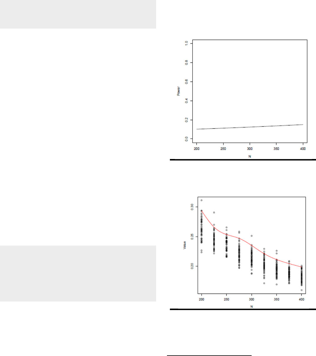
Power and accuracy

curves using sample sizes spanning 200-400 for the



 2relation are shown in Figures 3a and 3b.

Figure 3a. Power curve for Example 1 using

α = .05.

Figure 3b. Accuracy curve for Example 1 using

α= .05.

ncorporating a level of

assurance

(i.e., probability) of the

CI’s half-width study is a

differen

form of the AIPE

perspective

than

discuss

in the

urren

article. For more information about

it,

see

Kelley and Maxwell (2008).

Practical Assessment, Research & Evaluation, Vol 19, No 12 Page 9

Beaujean, Monte Carlo Sample Size Determination

# power curve of the X2-Y relation

plotPower(analysis.n, powerParam = "y~x2", alpha

= 0.05)

# accuracy curve of the X2-Y relation

plotCIwidth(analysis.n, c("y~x2"), assurance = 0.95)

An alternative to graphically displaying the results

is to use the

getPower()

findPower()

, and

getCIwidth()

functions. The first and third functions return the

power and CI widths, respectively, for each parameter

at the specified sample sizes (

nVal

). The second

function uses a

getPower()

object to find the sample

size for a given level of power. If the

findPower()

function returns the values Inf or NA, it means the

sample size values are too large or too small,

respectively, for that parameter at the specified power

level.

# find n for power of .80

power.n <- getPower(analysis.n, alpha=.05,

nVal=200:300)

findPower(power.n, iv="N", power=0.80)

# find CI half-widths when n=200

getCIwidth(analysis.n, assurance = 0.95,

nVal=200)/2

Example 2: Multiple Regression

With Data Quirks

For this second example, I add some quirks to the

data from Example 2. I only present models that

include one quirk, but combining multiple quirks in a

single model is a simple extension.

Data Quirk 1: Missing Data

Missing data is often a problem in research, so

conducting a sample size analysis without accounting

for missing data is often unrealistic (Graham, 2009).

For the current example, I made 20% of X

's data

missing completely at random (MCAR), but X

missing

values dependent on values of X

. Specifically, when

= 0, 15% of X

's data is missing; for each unit

increase and decrease in X

, the amount of missing data

increases and decreases, respectively. As long as I

include X

in the regression model, the missing values

for X

are missing at random (MAR).

simsem

has a variety of ways to include missing

data in the simulations, most of which use the

miss()

function. I use the logit method because it has the

ability to graph the amount of missing data. The logit

method requires a lavaan-like script that specifies how

much data should be missing for a given variable. Each

line of the script begins with a variable, then the

regression symbol (

), and then values for the amount

of missing data.

The values after the

are input for the inverse

logit function:

345















345











(5)

where a is the intercept, the bs are slope values,

and the Xs are predictor variables in the regression. For

example, if a = –1.38 and there are no predictors, then

the inverse logit value is 0.20, so approximately 20% of

the values should be missing. Likewise, if a = –1.73 and

b = 0.25, then approximately 15% of the values are

missing when X = 0, 19% of the values when X = 1,

and so forth.

# specify amount of missing data using logit

method

pcnt.missing <- '

# 20% of data missing

x2 ~ -1.38

# 15% of X1 data is missing when X3 is zero

x1 ~ -1.73 + 0.25

To plot the amount of missing data specified in

the logit equations, use the

plotLogitMiss()

function. The

plot for the current example is shown in Figure 4.

Figure 4 . Plot of missing data to include in

the simulated datasets for



and



# plot amount of missing data specified in the logit

equations

plotLogitMiss(pcnt.missing)

Practical Assessment, Research & Evaluation, Vol 19, No 12 Page 10

Beaujean, Monte Carlo Sample Size Determination

Having missing values requires determining how

to estimate the parameters in the presence of this

missingness. Only full information maximum

likelihood (FIML) and multiple imputation (MI) are

available estimation options in simsem, which can be

used with or without auxiliary variables. For details on

FIML, MI and auxiliary variables, see Enders (2011).

By default, simsem uses FIML when there are missing

values. To use MI requires two additional arguments:

the number of imputations for each data set (m) and

the R package to conduct the imputation (package)

Currently, only function from the mice (van Buuren &

Groothuis-Oudshoorn, 2011) and Amelia II (Honaker,

King, & Blackwell, 2011) packages can be used for the

imputation.

# FIML

missing.model.fiml <- miss(logit = pcnt.missing)

# MI

missing.model.mi <- miss(logit = pcnt.missing, m =

10, package = "mice")

# simulate regression data with missing data using

FIML

analysis.mis.237 <- sim(nRep=750,

model=analysis.model, n=237,

generate=pop.model, lavaanfun = "sem",

miss=missing.model.fiml, seed=565,

multicore=TRUE)

For the current example, I simulated the data with

n = 237 using FIML to handle the missing data. As I

included missing values, I increased m to 750. The

results are given in Table 4. The relative bias and

coverage values are within specified limits. Compared

to initial model (Example 1), power decreases slightly

for X

's and X

's regression coefficients and CI half-

widths for all thee predictors increase.

's regression coefficient is the smallest in value.

Thus, finding the sample size needed for it to be

estimated with power of 0.80, would mean that all

other regression coefficients would have at least a

power of 0.80. To find the sample size needed for X

regression coefficient to be estimated with power of

0.80, I use the same procedures described in finding an

unknown sample size for Example 1. As data are

missing, I specified the search to go from n = 200 to

The m

argumen

in the miss() function is not related to

number of simulated

samples

in the

study, m.

Table 4.

Values

From Monte Carlo

Sample Size

Studies.

Relativ

Bias

95%

Half-

Width

Pre-

dictor

Model

Value

Parameter

Cover-

age

Power

No Data Quirks (Example

0.66

0.01

0.04

0.96

1.00

0.15

0.05

0.09

0.00

0.95

0.12

0.30

0.01

0.02

0.95

0.99

0.14

Missing

Data with Full Information Maximum Likelihood

Estimation

0.66

0.00

0.03

0.96

1.00

0.18

0.05

0.06

0.02

0.95

0.09

0.15

0.30

0.01

0.95

0.94

0.17

’s Distribution with

Excess Skew

and Kurtosis

0.66

0.18

0.19

0.67

1.00

0.16

0.05

0.15

0.02

0.95

0.12

0.13

0.30

0.16

0.09

0.87

0.89

0.15

Unreliability of X

and

0.66

0.12

0.03

0.99

0.48

0.90

0.05

1.00

0.04

0.99

0.04

0.59

0.30

0.16

0.03

0.97

0.25

0.54

n = 5000, increasing by 200, and using m = 50

simulations per sample size. The results indicate that

when n = 3820 power is .80. I already showed that with

n = 237 the CI half-with is 0.15; increasing it to 3820

makes the CI half-width approximately 0.06.

# sample size study for X2 using FIML to handle

missing data

# simulate data from n=200 to n=5000 by 25

missing.n <- sim(nRep=NULL,

model=analysis.model,

n=rep(seq(200,5000,200), 50),

generate=pop.model, lavaanfun = "sem",

miss=missing.model.fiml, multicore=TRUE)

# power curve

plotPower(missing.n, powerParam="y~x2",

alpha=.05)

# accuracy curve

plotCIwidth(missing.n, c("y~x2"), assurance = 0.95)

# find n for power of .80

power.mis <- getPower(missing.n, alpha=.05)

findPower(power.mis, iv="N", power=0.80)

# find CI half-widths

getCIwidth(missing.n, assurance = 0.95,

nVal=3820)/2

As a point of comparison, I examined the sample

size required for a power of .80 using traditional

methods. Specifically, I used the G*Power program

Practical Assessment, Research & Evaluation, Vol 19, No 12 Page 11

Beaujean, Monte Carlo Sample Size Determination

(Faul, Erdfelder, Buchner, & Lang, 2009) and followed

the steps the authors outlined for a power analysis of a

single regression coefficient in a multiple regression

(what they call Deviation of a Single Linear Regression

Coefficient From Zero). The values I used for the G*Power

program and its output are in Figure 5, which shows

that the sample size needed is 2057.

One way to handle missing data in this situation is

to divide the sample size required for a complete

dataset by the proportion of observations thought to be

without missing values. Thus, if 20% of the

observations had missing values, then divide n by .80 to

find the final sample size estimate. Assuming that

between 20-30% of the data are missing makes the

required sample size between 2571-2939, likely making

the study underpowered for X

's effects.

Data Quirk 2: Non-Normality

One assumption in multiple regression is that the

residuals are normally distributed (Williams, Grajales, &

Kurkiewicz, 2013). There are a variety of ways for the

residuals to fail to meet this assumption, but a common

one is for the outcome variable to have a non-normal

distribution, such as when it has excessive skew or

kurtosis. For the current example, I made Y's skew

equal to negative four and its kurtosis equal to seven. A

plot of such a variable is in Figure 6.

Figure 6 . Kernel density plot of Y with skew =

–4 and kurtosis = 7.

simsem’s

bindDist()

function makes any of the

variables in the simulated data have the desired amount

of skew and kurtosis using the

skewness

and

kurtosis

arguments, respectively. Skew and kurtosis values need

to be included for each variable in the data. By setting

the

indDist

argument equal to the

bindDist()

object, the

sim()

function uses the specified skew and kurtosis

values.

# add skew and kurtosis to only to Y

distrib <- bindDist(skewness = c(-4,0,0,0), kurtosis

= c(7,0,0,0))

Figure

. G*Power

value specification

for

example

with

missing

data.

Practical Assessment, Research & Evaluation, Vol 19, No 12 Page 12

Beaujean, Monte Carlo Sample Size Determination

# simulate data with non-normal Y

analysis.nn.237 <- sim(nRep=10000,

model=analysis.model, n=237,

generate=pop.model, lavaanfun = "sem",

indDist=distrib, seed=565, multicore=TRUE)

The results of the MC simulations with a non-

normal Y variable are in Table 4. With m = 750, the

relative parameter bias values are outside of the

specified limits for all three variables, as is the relative

SE bias and coverage for X

, and the coverage X

. The

aberrant bias values decrease minimally with a m of

10,000, indicating that using a typical regression model

for this data will produce biased regression coefficients.

Compared to the results from Example 1, the power

decreased for X

and the 95% CI half-widths increased

for all three predictors. As X

's relative SE bias is

somewhat large, its CI will likely be inaccurate so the

half-width should be interpreted cautiously.

Data Quirk 3: Reliability

Another assumption of multiple regression is that

the variables are measured without error. While ideal,

this is seldom the case for measures of psychological

constructs. Not accounting for measurement

unreliability in the model results in biased parameter

estimates and a decrease in power (Cole & Preacher,

2014).

One way to account for variables measured

without perfect reliability is to use single-indicator

latent variables (Keith, 2006). Single-indicator latent

variables explicitly model a variable’s variance, which is

what is affected with unreliable measures. If :





is a

variable’s variance and ;



is the reliability of a

variable’s scores, then single-indicator latent variables

fix the variable’s error variance to (1–;



) :





, the true

variance to (;



) :





, and the path coefficients to one.

To make single-indicator latent variables more

concrete, say the reliability of the scores for X

and X

are both .70. Figure 7 contains a path diagram of the

regression model with these imperfectly-measured

variables. Note the addition of the error and true score

components for X

and X

. In addition, while the

correlation and regression coefficients are the same as

those from Example 1, the residual variance has

increased from 0.685 to 0.816 because the R

decreased

after modeling their unreliability.

Figure 7 . Path model using single-indicator latent

variables to account for the imperfect reliability of

and X

, which is .70 for both variables. T

represents the true score and E represents

measurement error. The new R

value can be

calculated via:

.66 × .7 × .66 + .05 × .70 × .05 + –.30 × 1 × –.30

+ (.66 × .40 × .05) × 2 + (.66 × .60 ×

–.30) × 2 + (.05 × .05 × –.30) × 2 = .184.

# data generating model with measurement error

pop.rel.model <-'

# measurement model

x1.true =~ 1

x2.true =~ 1

# for reliabilities of .70

# constrain error variances of X1 and X2 to be .30

x1 ~~ .3

x2 ~~ .3

# constrain true score variances of X1 and X2 to be

.70

x1.true ~~ .7

x1.true

x2.true ~~ .7

x2.true

# regression

y ~ 0.66

x1.true + 0.05

x2.true + -0.30

# predictor variables covariance

x1.true ~~ 0.40

x2.true + 0.60

x2.true ~~ 0.05

# residual variance

y~~ 0.816

# data analysis model accounting for measurement

error

analysis.rel.model <-'

Practical Assessment, Research & Evaluation, Vol 19, No 12 Page 13

Beaujean, Monte Carlo Sample Size Determination

# measurement model

x1.true =~ 1

x2.true =~ 1

# constrain error variances

x1 ~~ 0.3

x2 ~~ 0.3

# constrain true score variances

x1.true ~~ 0.7

x1.true

x2.true ~~ 0.7

x2.true

# predictor variables covariance

x1.true ~~ x2.true + x3 x2.true ~~ x3

# regression

y ~ x1.true + x2.true + x3

‘

# simulate data with unreliable variables

analysis.rel.237 <- sim(nRep = 750,

model=analysis.rel.model, n = 237,

generate=pop.rel.model, lavaanfun = "sem",

seed=565, multicore=TRUE

)

The results of the MC analysis are shown in Table

4. The relative parameter bias is a little high for X

and

, and very high for X

. When I set m = 5000, the

amount of relative parameter bias decreased to –.75 for

, indicating that even higher values of m might

produce better results for the MC study. The relative

SE bias and coverage are all within specified limits.

When compared to the values from Example 1, the

power for all three regression coefficients substantially

decreased and the 95% CI half-widths substantially

increased.

Discussion

In this article, I demonstrated the use of a Monte

Carlo (MC) study for the purpose of deciding on

sample size in regression models based on power and

accuracy in parameter estimation (AIPE). In the

examples, I used a multiple regression model with three

predictors and examined the sample size needed for

data without any quirks as well as data with missing

values, a non-normal outcome, and less-than-perfect

reliability. For the examples with no data quirks, the

results mapped directly onto the results from traditional

formula-based sample size determination methods.

When there are quirks in the data, however, there are

no simple formulae to determine sample size. The

results from the example MC studies showed that

ignoring these data quirks could result in underpowered

parameter estimation, inaccurate parameter estimates,

or both.

Unlike previous articles that showed how to use

MC studies to determine sample size, I focused on

regression models, since they are one of the most

common ways to analyze data (Troncoso Skidmore &

Thompson, 2010). In addition, I used the R statistical

language for all example analyses. As R is free and

available on many computer operating systems, the

procedures and R syntax in this article should be

readily usable by investigators for their own data

analysis.

Drawback of Using Monte Carlo Studies

While one of the purposes of this article was to

show the flexibility and benefits of the MC approach to

determining sample size, there is a drawback: it requires

users to know more about their studies’ variables than

traditional methods. Investigators have to specify not

onlyαand power, but they also have to specify values

for all the variables’ relations. Thus, Cohen’s (1992)

concern about researchers not knowing appropriate

effect size values for their particular field is amplified if

they have to know how all the variables relate to each

other. In the best situation, scholars would select the

model’s values from theory or previous research. In the

complete absence of any theoretical expectations,

Maxwell (2000) suggested starting with the assumption

that all zero-order correlations are .30, then changing

the values to see how it influences the required sample

size (i.e., sensitivity analysis). Using values of .30 gives

values around 0.14 (2 predictors) to 0.24 (10

predictors), which may or may not be appropriate for a

study.

Using the AIPE perspective adds yet one more

piece of information for the investigator to know: an

appropriate size for the CI half-width. There are

currently not any guidelines to determine the

appropriate CI half-width for a regression, but values

between 0.10 and 0.20 for standardized regression

coefficients are commonly used in the AIPE literature,

so are probably a good place to start. Of course, this

somewhat depends on the hypothesized value of the

regression coefficient. For example, narrower CIs are

likely better with coefficient values expected to be close

to zero in order to determine if the direction of the

effect is positive or negative. Likewise, if the coefficient

is expected to be large and well beyond some threshold

set for usefulness (e.g., a clinically-relevant effect), then

Practical Assessment, Research & Evaluation, Vol 19, No 12 Page 14

Beaujean, Monte Carlo Sample Size Determination

having a wider CI may be acceptable as long as its

bounds do not cross the threshold.

Monte Carlo Study Extensions

In the current article, I only focused on

determining the sample size for specific regression

coefficients. An alternative is to focus on the entire

model (i.e., omnibus) and base the sample size on the

value. This is easy to do using the simsem package

as the amount of error variance (i.e., 1–R

) is already

included as an estimated parameter in the output.

Another limitation of the models I used in this

article is that the outcome variable was continuous. The

same procedures could be used with variations of this

model, such as having categorical or count outcomes.

While this would require more complex models and

different effect sizes, the same basic procedures still

apply. Likewise, regression models with nested data

could also use this approach (e.g., Meuleman & Billiet,

2009).

References

American Educational Research Association. (2006).

Standards for reporting on empirical social science

research in AERA publications. Educational Researcher ,

35 , 33-40.

Bacchetti, P. (2010). Current sample size conventions:

Flaws, harms, and alternatives. BMC Medicine, 8 , 17.

Bacchetti, P. (2013). Small sample size is not the real

problem. Nature Reviews Neuroscience, 14 , 585-585. doi:

10.1038/nrn3475-c3

Barrett, P. (2007). Structural equation modelling: Adjudging

model fit. Personality and Individual Differences, 42 , 815-

824. doi: 10.1016/j.paid.2006.09.018

Beasley, W. H., & Rodgers, J. L. (2012). Bootstrapping and

Monte Carlo methods. In H. Cooper, P. M. Camic, D.

L. Long, A. T. Panter, D. Rindskopf, & K. J. Sher

(Eds.), APA handbook of research methods in psychology, Vol

2: Research designs: Quantitative, qualitative, neuropsychological,

and biological (pp. 407–425). Washington, DC: American

Psychological Association.

Beaujean, A. A. (2014). Latent variable modeling using

: A step-

by-step guide. New York, NY: Routledge/Taylor and

Francis.

American Psychological Association Publications and

Communications Board Working Group on Journal

Article Reporting Standards. (2008). Reporting

standards for research in psychology: Why do we need

them? What might they be? American Psychologist, 63 ,

839-851. doi: 10.1037/0003-066X.63.9.839

R Development Core Team. (2014).

: A language and

environment for statistical computing [Computer program].

Vienna, Austria: R Foundation for Statistical

Computing.

Boker, S. M., & McArdle, J. J. (2005). Path analysis and path

diagrams. In B. Everitt & D. C. Howell (Eds.),

Encyclopedia of behavioral statistics (Vol. 3, pp. 1529–1531).

West Sussex, England: Wiley.

Christensen, R. (2002). Plane answers to complex questions: The

theory of linear models (3rd ed.). New York, NY: Springer-

Verlag.

Cohen, J. (1988). Statistical power analysis for the behavioral

sciences (2nd ed.). Mahwah, NJ: Erlbaum.

Cohen, J. (1992). A power primer. Psychological Bulletin, 112 ,

155-159. doi: 10.1037/0033-2909.112.1.155

Cole, D. A., & Preacher, K. J. (2014). Manifest variable path

analysis: Potentially serious and misleading

consequences due to uncorrected measurement error.

Psychological Methods, 19, 300-315. doi:

10.1037/a0033805

Cumming, G. (2014). The new statistics: Why and how.

Psychological Science, 25 , 7-29. doi:

10.1177/0956797613504966

Cumming, G., & Finch, S. (2005). Inference by eye:

Confidence intervals and how to read pictures of data.

American Psychologist, 60 , 170-180. doi: 10.1037/0003-

066X.60.2.170

Descôteaux, J. (2007). Statistical power: An historical

introduction. Tutorials in Quantitative Methods for

Psychology, 3 (2), 28-34. Retrieved from

http://www.tqmp.org/Content/vol03-

2/p028/p028.pdf

Dupont, W. D., & Plummer, W. D., Jr.. (1998). Power and

sample size calculations for studies involving linear

regression. Controlled Clinical Trials, 19 , 589-601. doi:

10.1016/S0197-2456(98)00037-3

Enders, C. K. (2011). Applied missing data analysis. New York,

NY: Guilford.

Fan, X. (2012). Designing simulation studies. In H. Cooper

(Ed.), APA handbook of research methods in psychology (Vol.

3.): Data analysis and research publication (p. 427-444).

Washington, DC: American Psychological Association.

Faul, F., Erdfelder, E., Buchner, A., & Lang, A.-G. (2009).

Statistical power analyses using G*Power 3.1: Tests for

correlation and regression analyses. Behavior Research

Methods, 41 , 1149-1160. doi: 10.3758/brm.41.4.1149

Faul, F., Erdfelder, E., Lang, A.-G., & Buchner, A. (2007).

G*Power 3: A flexible statistical power analysis

Practical Assessment, Research & Evaluation, Vol 19, No 12 Page 15

Beaujean, Monte Carlo Sample Size Determination

program for the social, behavioral, and biomedical

sciences. Behavior Research Methods, 39 , 175-191. doi:

10.3758/bf03193146

Goodman, S. N., & Berlin, J. A. (1994). The use of predicted

confidence Intervals when planning experiments and

the misuse of power when interpreting results. Annals of

Internal Medicine, 121 , 200-206. doi: 10.7326/0003-

4819-121-3-199408010-00008

Graham, J. W. (2009). Missing data analysis: Making it work

in the real world. Annual Review of Psychology, 60 , 549-

576. doi: 10.1146/annurev.psych.58.110405.085530

Grissom, R. J., & Kim, J. J. (2005). Effect sizes for research: A

broad practical approach. Mahwah, NJ: Lawrence Erlbaum.

Hellmann, J. J., & Fowler, G. W. (1999). Bias, precision, and

accuracy of four measures of species richness. Ecological

Applications, 9 , 824-834. doi: 10.1890/1051-

0761(1999)009[0824:BPAAOF]2.0.CO;2

Hill, C. J., Bloom, H. S., Black, A. R., & Lipsey, M. W.

(2008). Empirical benchmarks for interpreting effect

sizes in research. Child Development Perspectives, 2 , 172-

177. doi: 10.1111/j.1750-8606.2008.00061.x

Honaker, J., King, G., & Blackwell, M. (2011). Amelia II: A

program for missing data. Journal of Statistical Software,

45(7), 1-47. Retrieved from

http://www.jstatsoft.org/v45/i07

Hoyle, R. H., & Smith, G. T. (1994). Formulating clinical

research hypotheses as structural equation models: A

conceptual overview. Journal of Consulting and Clinical

Psychology, 62 , 429-440. doi: 10.1037/0022-

006X.62.3.429

Keith, T. Z. (2006). Multiple regression and beyond. Boston:

Pearson.

Kelley, K. (2007). Methods for the Behavioral, Educational,

and Social Sciences: An R package. Behavior Research

Methods, 39 , 979-984. doi: 10.3758/BF03192993

Kelley, K., Lai, K., & Wu, P.-J. (2008). Using R for data

analysis: A best practice for research. In J. W. Osborne

(Ed.), Best practices in quantitative methods (pp. 535-572).

Thousand Oaks, CA: Sage.

Kelley, K., & Maxwell, S. E. (2003). Sample size for multiple

regression: Obtaining regression coefficients that are

accurate, not simply significant. Psychological Methods, 8 ,

305-321. doi: 10.1037/1082-989X.8.3.305

Kelley, K., & Maxwell, S. E. (2008). Sample size planning

with applications to multiple regression: Power and

accuracy for omnibus and targeted effects. In P.

Alasuutari, L. B. Bickman, & J. Brannen (Eds.), The Sage

handbook of social research methods (pp. 166-192).

Thousand Oaks, CA: Sage.

Kelley, K., & Maxwell, S. E. (2012). Sample size planning. In

H. Cooper, P. M. Camic, D. L. Long, A. T. Panter, D.

Rindskopf, & K. J. Sher (Eds.), APA handbook of research

methods in psychology, Vol 1: Foundations, planning, measures,

and psychometrics (pp. 181–202). Washington, DC:

American Psychological Association.

Marsaglia, G. (2003). Seeds for random number generators.

Communications of the ACM , 46 , 90-93. doi:

10.1145/769800.769827

Maxwell, S. E. (2000). Sample size and multiple regression

analysis. Psychological Methods, 5 , 434-458. doi:

10.1037/1082-989X.5.4.434

Maxwell, S. E., Kelley, K., & Rausch, J. R. (2007). Sample

size planning for statistical power and accuracy in

parameter estimation. Annual Review of Psychology, 59 ,

537-563. doi:

10.1146/annurev.psych.59.103006.093735

Meuleman, B., & Billiet, J. (2009). A Monte Carlo sample

size study: How many countries are needed for accurate

multilevel SEM? Survey Research Methods, 3 (1), 45-58.

Retrieved from http://ojs.ub.uni-

konstanz.de/srm/article/view/666.

Moher, D., Hopewell, S., Schulz, K. F., Montori, V.,

Gøtzsche, P. C., Devereaux, P. J., Altman, D. G.

(2010). CONSORT 2010 Explanation and Elaboration:

updated guidelines for reporting parallel group

randomised trials. Journal of Clinical Epidemiology, 63 , e1-

e37. doi: 10.1016/j.jclinepi.2010.03.004

Murphy, K. R., & Myors, B. (1998). Statistical power analysis: A

simple and general model for traditional and modern hypothesis

tests. Mahwah, NJ: Erlbaum.

Muthén, L. K., & Muthén, B. O. (2002). How to use a

Monte Carlo study to decide on sample size and

determine power. Structural Equation Modeling: A

Multidisciplinary Journal , 9 , 599-620. doi:

0.1207/S15328007SEM0904_8

Pornprasertmanit, S., Miller, P., & Schoemann, A. (2012).

simsem: SIMulated Structural Equation Modeling [Computer

software]. Retrieved from http://CRAN.R-

project.org/package=simsem

Rosseel, Y. (2012). lavaan: An R package for structural

equation modeling. Journal of Statistical Software, 48 (2), 1-

36. Retrieved from http://www.jstatsoft.org/v48/i02

Skrondal, A. (2000). Design and analysis of Monte Carlo

experiments: Attacking the conventional wisdom.

Multivariate Behavioral Research, 35 , 137-167. doi:

10.1207/S15327906MBR3502_1

Troncoso Skidmore, S., & Thompson, B. (2010). Statistical

techniques used in published articles: A historical

review of reviews. Educational and Psychological

Practical Assessment, Research & Evaluation, Vol 19, No 12 Page 16

Beaujean, Monte Carlo Sample Size Determination

Measurement, 70 , 777-795. doi:

10.1177/0013164410379320

van Buuren, S., & Groothuis-Oudshoorn, K. (2011).

Multivariate imputation by chained equations in R.

Journal of Statistical Software, 45 (3). Retrieved from

http://www.jstatsoft.org/v45/i03

Venables, W. N., Smith, D. M., & R Development Core

Team. (2012). An introduction to R. R Development

Core Team. Retrieved from http://cran.r-

project.org/doc/manuals/R-intro.pdf

Wilkinson, L., & American Psychological Association

Science Directorate Task Force on Statistical Inference.

(1999). Statistical methods in psychology journals:

Guidelines and explanations. American Psychologist, 54 ,

594-604. doi:10.1037/0003-066X.54.8.594

Williams, M. N., Grajales, C. A. G., & Kurkiewicz, D.

(2013). Assumptions of multiple regression: Correcting

two misconceptions. Practical Assessment Research and

Evaluation, 18 (11), 1-14. Retrieved from

http://pareonline.net/getvn.asp?v=18&n=11

Citation:

Beaujean, A. Alexander (2014). Sample Size Determination for Regression Models Using Monte Carlo

Methods in R. Practical Assessment, Research & Evaluation, 19(12). Available online:

http://pareonline.net/getvn.asp?v=19&n=12

Author:

A. Alexander Beaujean, Director

Baylor Psychometric Laboratory

Department of Educational Psychology

One Bear Place #97301

Waco, TX 76798-7301

Alex_Beaujean [at] Baylor.edu

http://blogs.baylor.edu/alex_beaujean